Deep Dynamic Neural Networks for Multimodal Gesture Segmentation ...

IEEE TRANSACTIONS ON PATTERN ANALYSIS AND MACHINE INTELLIGENCE, JANUARY 2016

1

Deep Dynamic Neural Networks for Multimodal Gesture Segmentation and Recognition Di Wu, Lionel Pigou, Pieter-Jan Kindermans, Nam Le, Ling Shao, Joni Dambre, and Jean-Marc Odobez Abstract—This paper describes a novel method called Deep Dynamic Neural Networks (DDNN) for multimodal gesture recognition. A semi-supervised hierarchical dynamic framework based on a Hidden Markov Model (HMM) is proposed for simultaneous gesture segmentation and recognition where skeleton joint information, depth and RGB images, are the multimodal input observations. Unlike most traditional approaches that rely on the construction of complex handcrafted features, our approach learns high-level spatio-temporal representations using deep neural networks suited to the input modality: a Gaussian-Bernouilli Deep Belief Network (DBN) to handle skeletal dynamics, and a 3D Convolutional Neural Network (3DCNN) to manage and fuse batches of depth and RGB images. This is achieved through the modeling and learning of the emission probabilities of the HMM required to infer the gesture sequence. This purely data driven approach achieves a Jaccard index score of 0.81 in the ChaLearn LAP gesture spotting challenge. The performance is on par with a variety of state-of-the-art hand-tuned feature-based approaches and other learning-based methods, therefore opening the door to the use of deep learning techniques in order to further explore multimodal time series data. Index Terms—Deep learning, convolutional neural networks, deep belief networks, hidden Markov models, gesture recognition.

F

1

I NTRODUCTION

I

N recent years, human action recognition has drawn increasing attention of researchers, primarily due to its potential in areas such as video surveillance, robotics, humancomputer interaction, user interface design, and multimedia video retrieval. Previous works on video-based action recognition focused mainly on adapting hand-crafted features [1], [2], [3]. These methods usually have two stages: an optional feature detection stage followed by a feature description stage. Well-known feature detection methods are Harris3D [4], Cuboids [5] and Hessian3D [6]. For descriptors, popular methods are Cuboids [7], HOG/HOF [4], HOG3D [8] and Extended SURF [6]. In the recent work of Wang et al. [9], dense trajectories with improved motion based descriptors and other hand-crafted features achieved state-of-the-art results on a variety of datasets. Based on the current trends, challenges and interests within the action recognition community, it is to be expected that many successes will follow. However, the very high-dimensional and dense trajectory features usually require the use of advanced dimensionality reduction methods to make them computationally feasible. Furthermore, as discussed in the evaluation paper by Wang et al. [10], the best performing feature descriptor is dataset dependent and no universal hand-engineered feature that outperforming all others exists. This clearly indicates that the ability to learn dataset specific feature extractors can be highly beneficial and further improve the current state-ofthe-art. For this reason, even though hand-crafted features have dominated image recognition in previous years, there has been a growing interest in learning low-level and midlevel features, either in supervised, unsupervised, or semisupervised settings [11], [12], [13].

D. Wu and L. Pigou contributed equally to this work.

Since the recent resurgence of neural networks invoked by Hinton and others [14], deep neural architectures have become an effective approach for extracting high-level features from data. In the last few years deep artificial neural networks have won numerous contests in pattern recognition and representation learning. Schmidhuber [15] compiled a historical survey compactly summarizing relevant works with more than 850 entries of credited papers. From this overview we see that these models have been successfully applied to a plethora of different domains: the GPUbased cuda-convnet implementation [16] , also known as AlexNet, classifies 1.2 million high-resolution images into 1000 different classes; multi-column deep neural networks [17] achieve near-human performance on the handwritten digits and traffic signs recognition benchmarks; 3D convolutional neural networks [18] [19] recognize human actions in surveillance videos; deep belief networks combined with hidden Markov models [20] [21] for acoustic and skeletal joints modelling outperform the decade-dominating paradigm of Gaussian mixture models in conjunction with hidden Markov models. Multimodal deep learning techniques were also investigated [22] to learn cross-modality representation, for instance in the context of audio-visual speech recognition. Recently Baidu Research proposed the DeepSpeech system [23] that combines a well-optimised recurrent neural network (RNN) training system, achieving the lowest error rate on a noisy speech dataset. Across the aforementioned research fields, deep architectures have shown great capacity to discover and extract higher level relevant features. However, direct and unconstrained learning of these complex models remains non-trivial, since the amount of training data required increases drastically with the complexity of the prediction model. It is therefore common practice to restrain the complexity of the model. This is generally done by operating on small patches to reduce the


input dimension and diversity [13], or by training the model in an unsupervised manner [12] such that more (unlabelled) data can be used, or by forcing the model parameters to be identical for different input locations as in convolutional neural networks [16], [17], [18]. Thanks to the immense popularity of the Microsoft Kinect [24] [25], there has been a surge in interest in developing methods for human gesture and action recognition from 3D skeletal data and depth images. A number of new datasets [26], [27], [28], [29] have provided researchers with the opportunity to design novel representations and algorithms and test them on a much larger number of sequences. While gesture recognition based on 3D joint positions may seem trivial, it is indeed not. This is due to several factors. First, there is the high dimensionality of the input and the huge variability with which the poses and movements are made. A second aspect that further complicates the recognition is the segmentation of different gestures. In practice segmentation is as important as the recognition, but it is an often neglected aspect of the current action recognition research, in which it is often assumed that pre-segmented sequences are available [4] [30] [31]. In this paper we aim to address these issues by proposing a data driven system. We focus on continuous acyclic video sequence labelling, i.e. video sequences that are nonrepetitive as opposed to longer repetitive activities, e.g. jogging, walking and running. By integrating deep neural networks within an HMM temporal framework, we can jointly perform online segmentation and recognition of this continuous stream of gestures. The proposed framework is inspired by the discriminative HMM, which embedded a multi-layer perceptron inside an HMM, and was used for continuous speech recognition [32] [33]. This manuscript is an extension of the works of [21], [34] and [35]. The key contributions can be summarized as follows: •

•

•

•

A Gaussian-Bernoulli Deep Belief Network is proposed to extract high-level skeletal joint features and the learned representation is used to estimate the emission probability needed to infer gesture sequences; A 3D Convolutional Neural Network is proposed to extract features from 2D multiple channel inputs like depth and RGB images stacked along the 1D temporal domain; Intermediate and late fusion strategies are investigated in combination with the temporal modelling. The results of both mechanisms show that multiple-channel fusions outperform individual modules; The difference of mean activations in intermediate fusion due to different activation functions is analyzed. This is a contribution itself, and should spur further investigation into effectively fusing various multi-model activations.

The remainder of this paper is organised as follows. Section II reviews related work on gesture recognition using temporal models and recent deep learning work on RGBD data. Section III introduces the formulation of our DDNN model and the intuition behind the high level feature extraction. Section IV details the model implementation. Section V presents the experimental analysis and Section VI concludes the paper with discussions related to future work.

2

2

R ELATED W ORK

Gesture recognition has drawn increasing attention from researchers, primarily due to its growing potential in areas such as robotics, human-computer interaction and user interface design. Different temporal models have been proposed. Nowozin and Shotton [36] proposed the notion of “action points” to serve as natural temporal anchors of simple human actions using a Hidden Markov Model. Wang et al. [37] introduced a more elaborated discriminative hidden-state approach for the recognition of human gestures. However, relying on only one layer of hidden states, their model alone might not be powerful enough to learn a higher level representation of the data and take advantage of very large corpora. In this paper, we adopt a different approach by focusing on deep feature learning within a temporal model. There have been a few works exploring deep learning for action recognition in videos. For instance, Ji et al. [19] proposed using 3D Convolutional Neural Network for automated recognition of human actions in surveillance videos. Their model extracts features from both the spatial and the temporal dimensions by performing 3D convolutions, thereby capturing the motion information encoded in multiple adjacent frames. To further boost the performance, they proposed regularizing the outputs with high-level features and combining the predictions of a variety of different models. Taylor et al. [11] also explored 3D Convolutional Networks for learning spatio-temporal features for videos. The experiments in [34] show that multiple network averaging works better than a single individual network and larger nets will generally perform better than smaller nets. Providing there is enough data, averaging multi-column nets [17] applied to action recognition could also further improve the performance. The introduction of Kinect-like sensors has put more emphasis on RGB-D data for gesture recognition but has also influenced other video-based recognition tasks. For example, the benefits of deep learning using RGB-D data have been explored for object detection or classification tasks. Dosovistskiy et al. [38] presented generic feature learning for training a Convolutional Network using only unlabeled data. In contrast to supervised network training, the resulting feature representation is not class specific and is advantageous on geometric matching problems, outperforming the SIFT descriptor. Socher et al. [39] proposed a single Convolutional Neural Net layer for each modality as inputs to multiple, fixed-tree RNNs in order to compose higher order features for 3D object classification. The single Convolutional Neural Net layer provides useful translational invariance of low level features such as edges and allows parts of an object to be deformable to some extent. To address object detection, Gupta et al. [40] proposed a geocentric embedding for depth images that encodes height above ground and angle with gravity for each pixel in addition to the horizontal disparity. This augmented representation allows CNN to learn stronger features than when using disparity (or depth) alone. Recently, the gesture recognition domain has been stimulated by the collection and publication of large corpora. One such corpus was made available for the ChaLearn


2013 competition in which HMM models were used by many participants: Nandakumar et al. [41] applied the MFCC+HMM paradigm for audio input while their visual module still relied on low level features such as Space-TimeInterest-Point (STIP) or covariance descriptor to process RGB videos and skeleton models. The 1st ranked team, Wu et al. [42], used and HMM model as audio feature classifier and Dynamic Time Warping as the classifier for skeleton features. A Recurrent Neural Network (RNN) was utilized in [43] to model large-scale temporal dependencies, for data fusion and for the final gesture classification. Interestingly, the system in [43] decomposed the gestures into a largescale body motion and local subtle movements. As a follow up, the ChaLearn LAP [44] gesture spotting challenge has collected around 14,000 gestures drawn from a vocabulary of 20 Italian gestures. The emphasis in this dataset is on user-independent online classification of gestures. Several of the top winning methods in the ChaLearn LAP gesture spotting challenge require a set of complicated handcrafted features for either skeletal input, RGB-D input, or both. For instance, Neveroa et al. [45] proposed a pose descriptor consisting of 7 subsets for skeleton features. Monnier et al. [46] proposed to use 4 types of features for the skeleton (normalized joint positions; joint quaternion angles; Euclidean distances between specific joints; and directed distances between pairs of joints). This was based on the features proposed by Yao et al. [47]) Additionally, he also used a histograms of oriented gradients (HOG) descriptor for RGB-D images around the hand regions. In [48], handcrafted features based on dense trajectories [9] are adopted for the RGB module. There is however also the trend to learn the features, in contrast to engineering them, for gesture recognition in videos. For instance, the recent methods in [34], [35] focused on single modality that used deep networks to learn representations from skeleton data and RGB-D data respectively. Neveroa et al. [45] presents a multi-scale and multimodal deep network for gesture detection and localization. Key to their technique is a training strategy that exploits i) careful initialization of the sub-components of individual modalities and ii) gradual fusion of modalities from the strongest to weakest cross-modality structure. One major difference to our proposed system is the treatment of time: rather than using a temporal model, they used frames within a fixed interval as the input of their neural networks. This approach requires the training of several multi-scale temporal networks to cope with gestures performed at different speeds. Furthermore, the skeleton features they used are handcrafted and whereas our features are learned from data.

3

M ODEL F ORMULATION

Inspired by the framework successfully applied to speech recognition [20], the proposed model is a data driven learning system. This results in an integrated model where the amount of prior knowledge and engineering is minimized. On top of that, this approach works without the need for additional complicated preprocessing and dimensionality reduction methods as that is naturally embedded in the framework.

3

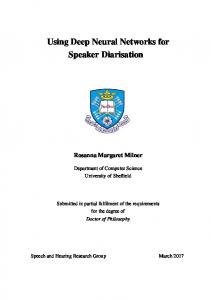
Fig. 1: Gesture recognition model: the temporal model is an HMM (left), whose emission probability p(Xt |Ht ) (right) is modeled by feedforward neural networks. Observations Xt (skeletal features Xts , or RGB-D image features Xtr ) are first passed through the appropriate deep neural nets (a DBN pretrained with Gaussian-Bernouilli Restricted Boltzmann Machines for the skeleton modality and a 3DCNN for the RGB-D modality) to extract high-level features (V s and V r ) . These are subsequently combined to produce an estimate of p(Xt |Ht ).

The proposed approach relies on a Hidden Markov Model (HMM) for the temporal aspect and neural networks to model the emission probabilities. In the remainder of this section, we will first present our temporal model and then introduce its main components. The details of the two distinct neural networks and fusion mechanisms along with post-processing will be provided in Section 4. 3.1

Deep Dynamic Neural Networks

The proposed Deep Dynamic Neural Networks can be seen as an extension of [21], where instead of only using the restricted Boltzmann machines to model human motion, various connectivity layers (fully connected layers, convolutional layers) are stacked together to learn higher level features justified by a variational bound [14] from different input modules. A continuous-observation HMM is adopted for modeling higher level temporal relationships. At each time step t, we have one observed random variable Xt composed of the skeleton input Xts and RGB-D input images Xtr as shown in the graphical representation in Fig. 1. The hidden state variable Ht takes on values in a finite set H composed of NH states related to the different gestures. The intuition motivating the HMM model is that a gesture is composed of a sequence of poses where the relative duration of each pose varies. This variance is captured by allowing flexible forward transitions within a Markov chain. In practice, Ht can be interpreted as being in a particular phase of a gesture a. Classically under the HMM assumption, the joint probability of observations and states is given by:

p(H1:T , X1:T ) = p(H1 )p(X1 |H1 )

T Y t=2

p(Xt |Ht )p(Ht |Ht−1 ),

(1) where p(H1 ) is the prior on the first hidden state, p(Ht |Ht−1 ) is the transition dynamics modeling the allowed state transitions and their probabilities, and p(Xt |Ht ) is the


4

using the max-sum algorithm also known as Viterbi algorithm. This algorithm searches the space of paths efficiently to find the most probable path with a computational cost that grows only linearly with the length of the chain [49]. ˆ t:T The result of the Viterbi algorithm is a path–sequence h of nodes going through the state diagram of Fig. 2 and from which we can easily infer the class of the gesture as illustrated in Fig. 8. 3.3

Fig. 2: State diagram of the ES-HMM model for low-latency gesture segmentation and recognition. An ergodic state (ES ) is used to model the resting position between gesture sequences. Each node represents a single state and each row represents a single gesture model. The arrows indicate possible transitions between states.

emission probability of the observation, modeled by Deep Neural Networks in our case. These elements are presented below. 3.2

State-transition model and inference

The HMM framework can be used for simultaneous gesture segmentation and recognition. This is achieved by defining the state transition diagram as shown in Fig. 2. For each given gesture a ∈ A, a set of states Ha is introduced to define a Markov model of that gesture. For example, for action sequence “tennis serving”, the action sequence can implicitly be dissected into ha1 , ha2 , ha3 as: 1) raising one arm 2) raising the racket 3) hitting the ball. More precisely, since our goal is to capture the variation in speed of the performed gestures, we set the transition matrix p(Ht |Ht−1 ) in the following way: when being in a particular node n at time t, moving to time t + 1, we can either stay in the same node (slower), move to node n + 1, or move to node n + 2 (faster). Furthermore, to allow the segmentation of gestures, we add an ergodic state (ES ) which resembles the silence state for speech recognition and serves as a catch-all state. From this state we can move to the first three nodes of any gesture class, and from the last three nodes of any gesture class we can move to ES . Hence, the hidden variable S S Ht can take values within the finite set H = ( a∈A Ha ) {ES}. Overall, we refer to the model as the ergodic states Hidden Markov Model (ES-HMM) for simultaneous gesture segmentation and recognition. It differs from the firing Hidden Markov Model of [36] in that we strictly follow a left-right HMM structure without allowing backward transition, forbidding inter-states transverse, assuming that the considered gestures do not undergo cyclic repetitions as in walking for instance. Once we have the trained model, we can use standard techniques to infer online the filtering distribution p(Ht |X1:t ), or offline (or with delay) the smoothed distribution p(Ht |X1:T ) where T denotes the end of the sequence. Because the graph for the Hidden Markov Model is a directed tree, this problem can be solved exactly and efficiently

Learning the emission probability

Traditionally, emission probabilities for activity recognition are learned by Gaussian Mixture Models (GMM). Alternatively, in this work we propose to model this term in a discriminative fashion. Since the input features are in high dimensionality, we propose to learn them using two distinctive types of neural networks each suited to one input modality, as summarized in the right of Fig. 1. Unfortunately, estimating a probability density such as an emission probability remains quite a difficult problem, especially in high dimensions. Strictly speaking, discriminative neural networks estimate posterior probabilities p(Ht |Xt ). Hence we should divide posteriors by priors p(Ht ) to obtain the emission probabilities p(Xt |Ht ) required by the HMM for decoding. However, using scaled likelihoods may not be beneficial if estimated priors do not match the priors in the test set [50]. Therefore, we employ the posteriors directly without dividing by the priors. This is equivalent to assuming that all priors are equal. Using this approach inference in the HMM depends only on the ratio between emission probabilities for the different states. One can interpret that the models are trained to directly predict the ratio between emission probabilities. This is similar to the approach used by Kindermans et al. to integrate transfer learning and an HMM-based language model into a single probabilistic model [51]. One should think of the predicted emission probability ratio as an unnormalized version of the true emission probability. Nevertheless, to simplify the discussion of our models for readers with a basic understanding of HMMs, we will refer to the predicted emission probability ratio simply as emission probabilities since the underlying model remains unchanged. For the skeletal features, we rely on a Deep-Belief Network (DBN) trained in two steps [52]: in the first step, stacked Restricted Boltzmann Machines (RBM) are trained in an unsupervised fashion using only observation data to learn high-level feature representations; in the second step, the model is used as a Deep-Belief Network whose weights are further fine-tuned for learning the emission probability. For the RGB and depth (RGB-D) video data, we rely on a 3D (2D for space and 1D for time) Convolutional Neural Networks (3DCNN) to model the emission probabilities. Finally, a fusion method combines the contributions of both modalities, this fusion can be done in an intermediate (hidden) layer or at a later stage at the output layer. In all cases (including the fusion), the supervised training is conducted by learning to predict the state label (an element of H) associated to each training or testing frame. Such an approach presents several advantages over the traditional GMM paradigm. First, while GMMs are easy to fit when they have diagonal covariance matrices and,


with enough components, can model any distribution, they have been shown to be statistically inefficient at modeling high-dimensional features with a complicated structure as explained in [20]. For instance, assume that the components of the input feature space can be factorized into two subspaces characterized by N and M significantly different patterns in the training data, respectively, and that the occurrences of these patterns are relatively independent1 . A GMM requires N ∗ M components to model this structure because each component must generate all the input features. On the other hand, a stacked RBMs model that explains the data only requires N + M components, each of which is specific to a particular subspace. This inefficiency of GMMs at modeling a structure that can be factorized leads to GMM+HMM systems having a very large number of mixture components,where each must be estimated from a very small fraction of the data. The approach for training the skeleton DBN model, starting with variational learning to train stacked RBMs with unlabeled data, followed by discriminative fine-tuning [52] has been shown to have several advantages. It has been observed that variational learning [14], which tries to optimize the data-likelihood while minimizing the KullbackLeibler divergence between the true posterior distribution of the hidden state (i.e. hidden layer variables of the RBMs in our case) and an approximation of this distribution, tends to produce unimodal distributions. This is beneficial, as this means that similar sensory inputs will be mapped to similar hidden variables. Thus, the intuition for using DBN for modeling the emission probability p(Xt |Ht ) from skeleton joints is that by learning the multi-layer network layer by layer, semantically meaningful high level features for skeleton configuration will be extracted while at the same time a parametric prior of human pose is learned. In our case, using the pairwise joints features as raw input, the data-driven approach network will be able to extract multijoint features relevant to the target classes. For instance, from the “toss” action data, a wrist joints rotating around shoulder joints feature is expected to be extracted from the backpropagation learning, and be the equivalent of those task specific ad hoc hard wired sets of joint configurations defined in [53] [54] [36] [55]. The benefit of such a learning approach is even more important when large amount of unlabeled data (e.g. skeleton data inferred from depth images of people performing unknown gestures) is available in addition to the labeled ones (this was not the case in this paper). Naturally, many of the features learned in this unsupervised way might be irrelevant for making the required discriminations, even though they are important for explaining the input data. However, this is a price worth paying if data availability and computation are cheap and lead to a stable mapping of the high-dimensional input into high-level features that are very good for discriminating between classes of interest. In this view, it is important to notice that each weight in a neural network is usually constrained by a larger fraction of the training samples than each parameter in a GMM, a point that has been masked by other differences in training. In 1. In our case, intuitively these spaces could be the features from different body parts, like left/right arm or torso features.

5

particular, neural networks have traditionally been training discriminatively, whereas GMMs are typically trained as generative models, which given their parametric nature partially compensates the fact that each mixture of a large GMM is usually trained on a very small fraction of the data. In summary, the feedforward neural networks offer several potential advantages over GMMs: • their estimation of emission probabilities does not require detailed assumptions about the data distribution; • they allow an easy combination of diverse features, including both discrete and continuous features; • they use far more of the data to constrain each parameter because the output on each training case is sensitive to a large fraction of the weights.

4

M ODEL I MPLEMENTATION

In this section, we detail the different components of the proposed Deep Dynamic Neural Network approach. 4.1

Ergodic States Hidden Markov Model

In all our experiments, the different modeling elements are specified as follows. The number of states NHa associated to an individual gesture has been set to 5. In total, the number of states is NH = 20 × 5 + 1 = 101 when conducting experiments on the ChaLearn dataset containing 20 classes. Note that intuitively, 5 states represent a good granularity as most gestures in the dataset are composed of 5 phases: an onset, followed by arm motions to reach a more or less static pose (often characterized by a distinct hand posture), and the motion back to the resting position. In future work, the optimization of the number of states2 and even a different number of states per gesture could be investigated. The training data of the ChaLearn competition is given as a set of sequences xi = [xi,1 , . . . , xi,t , . . . , xi,Ti ] where xi,t = [xsi,t , xri,t ]. Here, xsi,t corresponds to the skeleton and xri,t ] denotes the RGB-D input. As only a single gesture label is provided for each sequence, we need to define yi = [yi,1 , . . . , yi,t , . . . , yi,Ti ], the sequence of state labels yi,t associated to each frame. To do so, a forced alignment scheme is used. This means that if the ith sequence is a gesture a, then the first b T5i c frames are assigned to state h1a (the first state of gesture a), the following b T5i c frames are assigned to h2a , and so forth. For speech recognition community [56], a common approach is to adopt the trained GMM-HMM to revise the force-alignment labels and use them for the DNNs. Similary we could potentially adopt the same route. However, the contribution to the quality of the label might be trivial considering the increase of the training time. Hence, we argue that the adopted force-alignment scheme will suffice. Note that each gesture sequence comes with the video frames preceding and following the gesture. In practice, we extracted 5 frames before and after each gesture sequence and labeled them with the ergodic state (ES ) label. The transitional matrix p(Ht |Ht−1 ) was learned by simply collecting the transition statistics from the label sequences yi , allowing 5 frame jumps to accommodate skipping states. 2. Experiments with 10 states led to similar performance.


Fig. 3: Left: A point cloud projection of a depth image and the 3D positional features. Right: A DBN is trained to predict the emission probability p(Xts |Ht ) from the skeleton input ft . The double arrows indicate that the intermediate weights are first trained in an unsupervised fashion using stacked RBMs.

4.2

Skeleton Module

4.2.1 Skeleton input features Given our task, only the Nj = 11 upper body joints are relevant and considered, namely “ElbowLeft, WristLeft, ShoulderLeft, HandLeft, ElbowRight, WristRight, ShoulderRight, HandRight, Head, Spine, HipCenter”. The raw skeleton feas,N s,1 tures of time t are defined as xst = [xt , . . . , xt j ]. To capture the gesture dynamics, rather than using xst as raw input to our data driven approach, we follow the approach of [21] and compute the 3D positional pairwise differences of joints, as well as temporal derivatives, defined as (shown in Fig. 3) 3 : s,j ftcc = {xs,i t − xt |i, j = 1, 2, . . . , Nj ; i 6= j}

(2)

ftcp ftca

(3)

= =

{xs,i t+1 {xs,i t+1

−

xs,i t |i

−2×

= 1, 2, . . . , Nj }

xs,i t

+

xs,i t−1 |i

= 1, 2, . . . , Nj }

(4)

cp

This results in an input feature vector ft = [ftcc , ft , ftca ] N of dimension Nf = Nj × ( 2j + Nj + Nj ) ∗ 3 = 891. Admittedly, here we do not completely neglect human prior knowledge about information extraction for relevant static postures, velocity and acceleration of overall dynamics of motion data. While we have indeed used prior knowledge to define our relevant features, we believe they remain quite general and do not need dataset specific tuning. Note that the feature extraction process resembles the computation of the Mel Frequency Cepstral Coefficients (MFCCs) and their temporal derivatives typically used in the speech recognition community [20]. 4.2.2 Modeling Xts using Deep Belief Networks Given the input skeleton feature f , a DBN model is used to predict the emission probability, as shown in Fig. 3. The learning proceeds in two steps which we briefly mentioned in Section 3.3: in the first step, the network is considered to be a stack of RBMs, and trained using a greedy, layer-bylayer unsupervised learning algorithm [14]; in the second 3. Note that the offset features used in [21] depend on the first frame. Thus if the initialization fails which is a very common scenario, the feature descriptor will be generally very noisy. Hence, we do not use these offset features here.

6

step, a softmax network layer is added on top of the RBMs to create a DBN architecture, where the weights of the first step are used to initialize the corresponding weights in the DBN. The DBN is subsequently fine-tuned in a supervised manner to predict the emission probability. The number of nodes at each layer of the DBN are [Nf , 2000, 2000, 1000, NH ]. Below we give further details on the model and the training process. Gaussian-Bernoulli RBM. Restricted Boltzmann Machines (RBM) are undirected graphical models involving visible and hidden variables, with symmetric connections between the hidden and visible units of adjacent layers but without connections between units within the same layer. In most cases, the units in the RBMs model are binary random variables. However, in our case the visible unit in the first layer contains the vector of skeleton features f ∈ RNf , whose values are continuous. To be able to process this data, we resort to a Gaussian-Bernoulli RBM (GRBM) [52]. The main difference w.r.t. a standard RBM lies in the following: the energy term of the first layer f to the hidden binary stochastic units h ∈ {0, 1}F is given by: X (fi − bi )2 X X fi X W h − aj hj − ij j 2σi2 σi j=1 i i j (5) where θ = {W, b, a} are the free parameters. Here Wi,j serves as the symmetric synergy term between visible unit i and hidden unit j . The variables bi and aj specify the bias term of the visible and hidden units, respectively. The conditional distributions needed for inference and generative modeling are given by the traditional logistic function g for the binary hidden units, and the normal distribution N for the continuous units: X Wij fi + aj ) (6) P (hj = 1|f ) = g(

E(f , h; θ) = −

i

P (fi = f |h) = N (f |µi , σi2 ). (7) P where µi = bi + σi2 j Wij . In practice, we normalize the data (mean subtraction and standard deviation division) in the preprocessing phase. Hence, instead of learning σi2 , one typically uses σi2 = 1 during training. We ran 100 epochs using a fixed recipe-based on stochastic gradient descent with a mini-batch size of 200 training cases to train the stacked RBM. The learning rate is fixed to 0.001 for the Gaussian-Bernoulli RBMs, and to 0.01 for the higher-layer binary-binary RBMs. DBN forward training. The DBN is initialized with the result of the previous pretraining. The goal of this initialization is to avoid suboptimal local minima and to increase the network’s generalization capabilities. The learning rate for the parameter fine tuning starts at 1 with 0.99999 minibatch scaling. During the experiments, early stopping occurs around epoch 440. The optimization completes with a frame-based validation error rate of 16.5%. 4.3

RGB & Depth 3D Module

4.3.1 Preprocessing DeepMind [57] presented the first deep learning model to successfully learn control policies directly from highdimensional sensory input using deep reinforcement learn-


7

Fig. 4: 3DCNN architecture. The input is 2 × 2@64 ∗ 64 ∗ 4, meaning 2 modalities (depth and RGB) for the hand and body regions, each being 4 consecutive 64 by 64 frames stacked together. See text for further details. ing. However, working directly with raw input Kinect recorded data frames, which are 640 × 480 pixel images, is computationally very demanding. Therefore, our first step in the preprocessing stage consists of cropping the image to the highest hand and the upper body-based on the given joint information. In the ChaLearn dataset, we determined that the highest hand is the most interesting. When both hands are used, they tend to perform the same (mirrored) movement, When only one hand is used, it is always the highest one which is relevant for the gesture. Furthermore, to be invariant to handedness, we train the model with the right hand view. For this reason, the video was mirrored when the left hand is actually the performing hand. The preprocessing results in four video samples (body and hand with grayscale and depth) of resolution 64 × 64. Furthermore, the noise in the depth maps is reduced by removing the background using the automatically produced segmentation mask provided with the data, and applying a median filtering. Depth images are Z-normalized (the mean is subtracted as it is rather irrelevant to the gesture subclass and the result divided by the standard deviation), whereas RGB images are only normalized by the image standard deviation. The outcome is illustrated in Fig. 5. 4.3.2 3DCNN Architecture This architecture consists of a series of layers composed of either convolution, pooling or fully connected layers. The 3D convolution itself is achieved by convolving a 3D kernel to the cuboid formed by stacking multiple contiguous frames together. We follow the nomenclature of [19]. However, instead of using tanh units as in [19], Rectified Linear Units (ReLUs) [16] were used to speed up training. Formally, the value of a unit at position (x, y, z) (z here corresponds to the time-axis) in the j -th feature map in the i-th layer, xyz denoted as vij , is given by: xyz vij

The complete 3DCNN architecture is depicted in Fig. 4: 4 types of input contextual frames are stacked as size 64 × 64 × 4 (as illustrated in Fig. 5). The first layer (H1) consists of 32 feature maps produced by 5 × 5 spatial convolutional kernels, followed by local contrast normalization (LCN) [58]. Note that the filter response maps of the Depth and RGB images of the hand (and body) are summed to produce a single feature map, thus resulting in H1 32 feature maps for each of the hand and for the body region. A 3D max pooling with strides (2, 2, 2) is then applied. The second layer uses 64 feature maps with 5 × 5 kernels followed by LCN and 3D max pooling with strides (2, 2, 2). The third layer is composed of 64 feature maps with 4 × 4 kernels followed by 3D max pooling with strides (1, 2, 2). All hand and body convolutional layer outputs of H6 are flattened in H7, and fed into one fully connected layer of size 1024. Finally, the output layer has NH values, the number of states in the HMM state diagram (see Fig. 2). 4.3.3 Details of Learning During training, dropout [59] is used as the main regularization approach to reduce overfitting. Nesterov’s accelerated gradient descent (NAG) [60] with a fixed momentumcoefficient of 0.9 and mini-batches of size 64 are also used. The learning rate is initialized at 0.003 with a 5% decrease after each epoch. The weights of the 3DCNN are randomly initialized from a normal distribution with µ = 0 and σ = 0.04. The frame-based validation error rate is 39.06% after 40 epochs. Compared with the skeleton module (16.5% validation error rate), the 3DCNN has a notable higher frame-based error rate.

4.3.4 Looking into the Networks: Visualization of the Filter Banks The convolutional filter weights of the first layer are depicted in Fig. 5. The unique characteristics from the kernels Q −1 P −1 R −1 i i i X X X X pqr (x+p)(y+q)(t+r) = max(0, (bij + wijm v(i−1)m )) are clearly visible: as hand input images (RGB and depth) have larger homogeneous areas than the body inputs, the m p=0 q=0 r=0 (8) resulting filters are smoother than their body-processing


8

counterparts. In addition to being smoother overall than the grayscale filters, depth filters also exhibit stronger edges. A similar finding was reported in [39]. Finally, when looking at the joint depth-image response maps, we notice that some filters better capture segmentation-like information, while others are more edge-oriented. 4.4

Multimodal Fusion

To combine the two modalities, two strategies can be used, as shown in Fig. 6: a late fusion approach and an intermediate fusion approach. 4.4.1 Late Fusion This scheme combines the emission probabilities estimated from the different input as a simple linear combination:

p(Xt |Ht ) ∝ α · p(Xts |Ht ) + (1 − α) · p(Xtr |Ht )

(9)

Here, the different emission probabilities are provided by the modules described in 4.2 and 4.3. The coefficient α controls the contributions of each source and its value is optimized through cross validation. Interestingly, the best performing α is very close to 0.5, indicating that both modalities are equally important.

Fig. 6: Multimodal dynamic networks with late fusion scheme (left) and intermediate fusion scheme (right). The late approach simply combines the emission probabilities from two modalities. In the intermediate fusion scheme, each modality (skeleton and RGB-D) is first pretrained separately, and their high-level representation V s and V r (the penultimate node layers of their neural networks) are concatenated to generate a shared representation. The two sub-modules in the resulting architecture are trained jointly.

5.1

ChaLearn LAP Dataset

4.4.2 Intermediate Fusion As an alternative to the late fusion scheme, we can take advantage of the high-level representation learned by each module (and represented by the V s and V r nodes of the penultimate layer of the respective networks, i.e. the layer before the softmax output). To do this, we fuse the modalities in an intermediate fashion by concatenating these two layers in one layer of 2024 hidden unites. Then we learn a cross-modality emission probability directly from the resulting network. Note that this is very similar in spirit to the approach proposed in [22] for audio-visual speech recognition. An important difference is that in [22], the same stacked RBMs/DBN architecture was used to represent both modalities before the fusion, whereas in our case, a stacked RBMs/DBN and a 3DCNN are used. The resulting architecture is trained as follows. We start by first initializing the weights of the deeper layers from the previously trained sub-modules. Afterwards, we jointly fine tune the whole network (including the last layer parameters). The training ends when the validation error rate stops decreasing (∼15 epochs). We argue that using the “pretrained” parameters is important due to the heterogeneity of the inputs of the system. Furthermore, the joint training is included to adjust the parameters to be able handle the heterogeneity and produce to produce a more reliable estimate from the multimodal data.

The dataset used in this work was made public for the ChaLearn LAP [44] gesture spotting challenge4 . The focus is on “multiple instance, user independent spotting” of gestures, which means learning to recognize gestures from several instances for each category performed by different users. The gestures contained in this dataset are 20 Italian cultural/anthropological signs. The challenge dataset contains 940 video sequences, each performed by a single person and composed of 10 to 20 gesture instances, totaling about 14, 000 individual gestures. There are 20 gesture classes, i.e. vattene, vieniqui, perfetto, furbo, cheduepalle, chevuoi, daccordo, seipazzo, combinato, freganiente, ok, cosatifarei, basta, prendere, noncenepiu, fame, tantotempo, buonissimo, messidaccordo, sonostufo, with the number of samples well balanced between classes. The average length of gestures is 39 frames, the minimum frame number for a gesture is 16 and the maximum frame number is 104. This dataset is challenging because of the “user independent” setting. Some of gestures differ primarily in hand pose but the overall arm motions can be quite similar as illustrated in Fig. 7. In terms of data, three modalities are provided with the input videos: the sequence of skeleton joints, and the RGB and depth images (including a segmentation of the person performing the gesture).

5

5.2.1 Training and evaluation protocol We follow the ChaLearn experimental protocol, in which the input sequences are split into 700 videos for training, and 240 sequences for testing. Note that the test sequences are not segmented a priori and the gestures must be detected within a continuous data stream which, in addition to the

E XPERIMENTS AND A NALYSIS

This section reports the experiments performed to validate our model. First, we will introduce the ChaLearn dataset, and then present the experimental protocol we followed. In Section 5.3, we will present and analyze the obtained results, including a discussion on the modeling elements. Finally, Section 5.4 will briefly discuss the computational complexity of the approach.

5.2

Experimental protocol

4. http://gesture.chalearn.org/2014-looking-at-peoplechallenge/data-2014-challenge


9

Fig. 5: Visualization of input frames, first convolutional layer 5 × 5 filters, and corresponding response maps. As depth images are smoother than the grayscale ones, the corresponding filters are smoother as well.

performance measure known as the Jaccard index, which relies on a frame-by-frame prediction accuracy. More precisely, if GTi denotes the sequence of ground truth labels in video i, and Ri the algorithm output, the Jaccard index of the video is defined as: (a) “Perfetto”

(b) “Perfetto”

(c) “Buonissimo”

and JIi =

(d) “OK”

(g) “Basta”

(e) “Non ce ne piu” (f) “Combinato”

(h) “Cheduepalle”

(i) “Daccordo”

Fig. 7: Examples of gestures in the ChaLearn dataset. This dataset is challenging because of the “user independent” setting (a)&(b), some of gestures differ primarily in hand pose but not in the arm movement (d)&(e). Some gestures require both hands to perform (g,h,i). Subtle hand movement (c) and differences in execution speed and range (f) also make this recognition task challenging.

targeted gestures, also contains noisy and out-of-vocabulary gestures. Furthermore, in the experiments, we split the training videos into 650 videos for training the neural network parameters, and 50 videos are used as validation for monitoring the training performance and the optimization of the hyper-parameters. 5.2.2

Performance measures

Several measures can be used to evaluate the gesture recognition performance. In this work, we adopted the ChaLearn

Ns (GTi , Ri , g) , Nu (GTi , Ri , g) X JIi (GTi , Ri , g)

JIi (GTi , Ri , g) =

1 |Gi )| g∈G

(10) (11)

i

where Ns (GTi , Ri , g) denotes the number of frames where the ground truth and the prediction agree on the gesture class g . The quantity Nu (GTi , Ri , g) reflects the number of frames labeled as a gesture g by either the ground truth or the prediction, and Gi denotes the set of gestures either in the ground truth or detected by the algorithm in sequence i5 . The average of the JIi over all test videos is reported as the final performance measure. Note that experimentally, this measure tends to penalize false positives less than missing true positives. Being defined at the frame level, the Jaccard index can vary due to variations of the segmentation (both in the ground truth and recognition) at gesture boundaries, which can be irrelevant from an application viewpoint. For this reason, we also used the performance at the gesture event level by following the commonly used PASCAL challenge intersection over union criterion. If for a gesture segment G∩R > 0.5, where R denotes a recognized G, we have G∪R gesture segment of the same class, then the gesture is said to be recognized. However, if this also holds for a gesture segment of another class, the prediction is said to be incorrect. Otherwise the gesture is rated as undetected. This allows us to define the Recognized, Confused and Missed performance measures at the video level. These quantities are then averaged over the test sequences for reporting. 5. Note that ’non gesture’ frames are excluded from the counts.


10

Fig. 8: Viterbi decoding of sample sequence #700, using skeleton (top), RGB-D (middle) and late fusion system (bottom). The x-axis represents time and the y-axis represents the hidden states of all classes and of the ergodic state (state 101) constituting the finite set H. The cyan lines represent the Viterbi shortest path, while red lines denote the ground truth labels, and the yellow segments are the predicted labels. The fusion method exploits the complementary properties of individual modules, e.g. around frame 200 the skeleton help solving the missed detection from the 3DCNN module, while around frame 1450, the 3DCNN module can help suppress the false positive prediction made by the skeleton module. Module

Skeleton – DBDN RGB-D – 3DCNN Multimodal Late Fusion Multimodal Inter. Fusion

Validation 0.783 0.752 0.817 0.800

Test 0.779 0.717 0.809 0.798

Skeleton - DBDN

RGB-D - 3DCNN

TABLE 1: Results in terms of Jaccard index JI for the different network structures and modalities modeling the emission probabilities.

5.2.3

Tested systems

We evaluated the recognition performance made by the HMM applied to the emission probabilities estimated from either the skeleton data, the RGB-D image data, the late fusion scheme, and the intermediate fusion scheme. Note that in all cases the HMM output was further filtered to avoid false alarms, by considering gesture segments of less than 20 frames as noise and discarding them. 5.3

Results

Overall results. The performance measurements of the algorithms are given in Tables 1 and 2. As can be observed from both performance measures, the skeleton module usually performs better than the RGB-D module. In addition, its generalization capability is better than that of the RGB-D module, especially when measured with the Jaccard index where there is almost no drop of performance between the validation and the test data. One possible explanation is that the information in the skeleton data is more robust, as it benefited from training using huge and highly varied data [24]: around on million images from both realistic and synthetic depth images were used to train the decision forest classifiers involved in the joints extraction. On the other hand, as the RGB-D module relies on the raw data and was learned only from the ChaLearn training set, it may suffer from some overfitting. Another interesting conclusion that can be drawn from Table 2 is that while most errors from the RGB-D module are due to under detection (the Missed rate is 19.7%, whereas it is only 4.1% for the skeleton), the skeleton

Multimodal Late Fusion Multimodal Inter. Fusion

% Recognized Confused Missed Recognized Confused Missed Recognized Confused Missed Recognized Confused Missed

Validation 86.3 11.4 2.3 78.7 5.2 16.1 87.9 9.1 3.0 86.5 7.3 6.2

Test 83.6 12.3 4.1 75.8 4.5 19.7 86.4 8.7 4.9 85.5 6.8 7.7

TABLE 2: Gesture classification performance at the event level, as a percentage of the number of gestures.

module is more reactive to gesture activity, but makes more mistakes (the Confused rate is 12.3% vs 4.5% for RGB-D). Finally, the results also demonstrate that the combination of both modalities is more robust, as shown by increase in the recognition rate and the reduced drop in the generalization capability (for instance the decrease of the Recognized rate is lower than for the skeleton data alone). Confusion matrices. The confusion matrices (in log-form) in Fig. 9 better illustrate the complementarity of the behaviours of the two modalities. The higher under-detection rate of RGB-D is immediately apparent (whiter matrix, except for last ’undetected’ column). We can also notice that some gestures are more easily recognized than others. This is the case of the “Basta” gesture, whose arms motion resembles the start and end of the arm motion of many other gesturess (see Fig. 7). Regardless the modality, the model tends to recognize only a few instance of the other gesture classes, whenever their likelihoods are low when being evaluated using the HMM states associated with their true label. This is probably due to too much variability in the execution of the gesture. Similarly, the hand movement and pose of the “Buenissimo” gesture is present in several other gesture classes. As a result, their instances are often confused with “Buenissimo” when relying solely on the skeleton informa-

True

undetected

vattene vieniqui perfetto furbo cheduepalle chevuoi daccordo seipazzo combinato freganiente ok cosatifarei basta prendere noncenepiu fame tantotempo buonissimo messidaccordo sonostufo



100

10-1

10-2

10-3

Predicted

True

undetected


(a) Skeleton - DBN


100

10-1

10-2

10-3

Predicted

True


undetected


(b) RGB-D - 3DCNN

100

10-1

10-2

Predicted

10-3

(c) Multimodal Late Fusion

Fig. 9: Confusion Matrices (log-form) for the different modalities.

tion. However, as these gestures differ primarily in their hand pose, this confusion is reduced by using the RGB-D domain, or by fusing the skeleton and RGB-D modules. The complementary properties of the two modalities are also illustrated by the Viterbi path decoding plot in Fig. 8. In general, the benefit of the complementarity between arm pose/gesture and hand pose can be observed from the whiter confusion matrix than in the skeleton case (less confusion due to hand pose information from RGB-D) and much less under-detection than for the pure RGB-D model (thanks to an improved upper-body pose discrimination

11

thanks to skeleton input). However, the single modalities have more difficulties in correcting the recognition errors which are due to variations coming from the performer, like differentiating gestures from people that gesticulate more (see Fig. 11). Late vs. Intermediate fusion. The results in Tab. 1 and 2 show that the intermediate fusion system improved individual modalities, but without outperforming the late fusion strategy. The result is counter-intuitive, as we would have expected the cross-modality learning in the intermediate fusion scheme to result in better emission probability predictions, compared to the simple score fusion in the late system. One possible explanation is that the independence assumption of the late scheme better preserves both the complementarity and redundancy of the different modalities, properties which are important for fusion. Another possible explanation is that in the intermediate fusion learning process, one modality may dominate and skew the network towards learning that specific module and lowering the importance of the other one. The large difference between the mean activations of the skeleton module neurons which are predominantly larger than those of the RGB-D ConvNet’s (0.57 vs. 0.056) can be an indicator of such a bias during the multimodal fine-tuning phase and support this conjecture, even if these mean activations are not directly comparable due to the neuron heterogeneity: the skeleton DBN has logistic units whereas the 3DCNN has rectified linear units (ReLUs). Note that such heterogeneity was not present when fusing modalities in [22] where better registration and less spatial registration variability in lip images allowed the authors to resort to the stacked RBMs for both the visual and auditory modality. Based on these observations, further investigation on how to handle heterogeneous networks and the fusion of multimodal data could be an interesting research direction. HMM benefit. As the emission probabilities are learned in a discriminative manner, one could wonder whether the HMM brings any benefit beyond smoothing. To investigate this, we removed the HMM model and performed the smoothing as follows: for a given gesture a, we computed its score at time t, Score(a, t), by summing the emission probabilities p(Xt |Ht = h) for all nodes associated to that gesture, i.e. h ∈ Ha . This score is then smoothed in the temporal domain (using a window of 5 frames) to obtain \ a, t). Finally, following [61], the gesture recognition Score( is performed in two steps: first finding gesture segments by thresholding the score of the ergodic state; then, for each resulting gesture segment, the recognized gesture is defined as the one whose average score within the segment is maximal. Fig. 10 visualizes the predictions for the different temporal smoothing strategies. In general, we could observe that better decisions on the presence of gestures and improved localization of the gesture boundaries are obtained with the proposed DDNN. This is due to the use of the temporal model defined in Fig. 2. On the other hand, the gesture detection based on a simple threshold is rather unstable and much more sequence dependent. As a result, the overall performance of the simplified decoding scheme without the HMM temporal reduces the performance to JI = 0.66, while the Recognized,


(a) Sample #806

(b) Sample #702

Fig. 11: Examples of performer variations in the upper body dynamic. Most performers tend to keep their upper-body static while performing the gesture, leading to good recognition performance (Jaccard index of person on the top is 0.95 for the late fusion system). Some persons are more involved and move more vehemently (person at the bottom, Jaccard index of 0.61), which can affect the recognition algorithm itself (bottom left samples) or even the skeleton tracking (bottom right; note that normally cropped images are centered vertically on the head position).

Confused and Missed corresponding to Table 2 for the test set are 76.6 , 5.3 and 18.1. However, note that the this simple method relying on just the gesture probabilities predicted by the neural networks on 5 frame inputs still outperforms the Jaccard index of 0.413 obtained by [62] when using a 5 frames template matching system using handcrafted features. Comparison with the state-of-the-art. The performance of other state-of-the-art techniques is given in Table 3. The first half of the table uses hand crafted feature representations that are subsequently classified. Our proposed system performs on par with the top two methods. However, hand crafted feature methods’ performance are unlikely to improve much as more training data becomes available. The representation learning methods in the second half of the Table perform comparably with the best hand crafted feature approaches and the top representation method achieves the best Jaccard index score. Given more training data, it is expected that these networks will be able to become even better suited to the “user independent” setting. It also worth noting that our proposed system is the only method that incorporates more structured temporal modeling. The other approaches resort to a more basic sliding window approach. We believe this is an interesting research direction because an HMM-like approach can be adapted to various lengths of gestures and exploit temporal structure better. 5.4

Computational Complexity

We can distinguish between two complexities: the training complexity, and the test complexity. Complexity at training time. Although training deep neural network using stochastic gradient descent is computationally intensive, the reuse of pretrained network parameters, as done in our case, can help to speed up the learning process because the improved initialization leads to faster convergence. We can observe differences in training time as a function of the modality (and architecture). Specifically, using a modern GPU (GeForce GTX TITAN Black) and the

12

Module Skeleton RGB-D Fusion [46] 3 set skeletal & HOG, Boosted classifier 0.791 0.822 [63] 3D skeletal pose & HOG, MRF 0.790 0.827 [48] Dense trajectory (HOG, HOF, MBH) 0.792 [62] Template-based Random Forest Classifier 0.747 [64] Fisher Vector, Dynamic Programming 0.745 [65] Independent Subspace Analysis, RF 0.649 [66] PHOG, SVM, HMM 0.454 0.462 0.597 [45] Representation Learning (multiscale) 0.808 0.809 0.849 [35] CNN 0.789 [34] Deep Neural Networks 0.747 0.637 0.804 DDNN (this work) 0.779 0.717 0.809

TABLE 3: Comparison of results in terms of the ChaLearn Jaccard index with state-of-the-art related works.

conv op. implemented by Theano [67], the training time per epoch of the DBN skeleton module is less than 300 seconds. This allows us to complete the 500 training epochs in just 2 days. The training time of each epoch of the 3DCNN RGB-D module is much longer. Each epoch requires more than 10,000 seconds, which results in a total training time of about 5 days for 40 epochs. Because the multimodal network is being initialized with the individual subnetwork parameters, its training time is only half that of the standalone 3DCNN. Complexity at test time. Given the trained models, our framework can perform real-time video sequence labeling on the GPU, thanks to the low cost of inference. More specifically, a single feedforward neural network incurs linear computational time (O(T )). Furthermore, it can be implemented very efficiently on the GPU because because it requires mainly matrix products and convolutional operations. The computational complexity of the Viterbi algorithm is O(T ∗ |S|2 ), where T is the number of frames and |S| the number of states, and can be executed in real-time given our state-space. In practice, our multimodal neural network can be deployed at 90 FPS. Remarkably, the preprocessing steps take most of the time and an unoptimized version runs already at 25 FPS, while the Viterbi decoding runs at 90 FPS. Hence, with further optimizations the complete system can achieve faster than real-time performance.

6

C ONCLUSION AND FUTURE WORK

In this paper, we presented a novel Deep Dynamic Neural Network for continuous gesture recognition on multimodal data comprising image and depth (RGB-D) data and skeleton features. In contrast to previous state-of-the-art methods, we do not rely on handcrafted features that are timeconsuming to engineer, especially when this has to be done for each input modality independently. Instead we utilize deep neural nets to automatically extract the relevant information from the data. Because the input data is multimodal, our model integrates two distinct feature learning methods, (1) Deep Belief Networks for the processing of skeleton features and (2) 3D Convolutional Neural Networks for RGB-D data. On top of that, we extended our feature learning model with an HMM to incorporate temporal dependencies. This compound model jointly segments and classifies the multimodal datastream. This contrasts with most prior work, where the segmentation was assumed to be known a priori.


13

Fig. 10: HMM temporal contribution. First row: output emission probabilities for each gesture as given by the late fusion scheme (see text) for the test set #703. The dashed line represents the probability of the Resting/Other gesture state, while other color represent different gestures. Second row: resulting recognized gestures, without HMM modeling. Third row: HMM output. Fourth row: ground truth segmentation. Without temporal modeling, the decision boundary of a gesture will be more rugged and it is more difficult to make hard decisions of where the gesture starts or ends. Hence, in general, it causes miss-detection and missmerging. Thanks to the HMM temporal modeling and Viterbi path decoding, gesture boundaries are usually cleaner defined from the Resting state to the gesture states, resembling the behavior of the manual annotators with better accuracy.

We evaluated this model on the ChaLearn LAP dataset and have shown the following. First, multimodal fusion of the different inputs results in a clear improvement over unimodal approaches due to the complementary nature of the different input modalities. Skeleton features are very good for segmentation but make more mistakes during recognition, RGB-D features on the other hand allow for reliable recognition but are not as good for segmentation. Second, the integration of a more complex temporal model (the HMM) outperforms averaging of the outputs, hereby demonstrating that the temporal structure of the data can be well exploited. Third, Our experimental validation on the ChaLearn LAP dataset has indicated that our method performs at the same level as other state-of-the-art methods. There are several directions for future work. With the increase in the availability of dedicated processing units such as GPUs, feature learning models will only become more prevalent. For this reason, the study of multimodal approaches that extract complementary representations from heterogeneous inputs, as done in [61], needs more exploration. Furthermore, the integration of HMM is one of the many ways to take the temporal structure into account. Therefore, it would be interesting to verify whether the performance can be improved further by the integration of other probabilistic models such as conditional random fields or even more advanced variants [37]. A second promising research path would be to build a unified neural network to make better use of the temporal component of the problem. For example by using Recurrent Neural Networks, possibly with long short-term memory [68] nodes.

ACKNOWLEDGEMENT The authors would like to thank Sander Dieleman for his guidance in building, training and initializing Convolutional Neural Networks. This project has received funding from

the European Unions Horizon 2020 research and innovation programme under the Marie Sklodowska-Curie grant agreement NO 657679 and BMBF (01GQ1115). This work was also supported in part by National Natural Science Foundation of China under Grant 61528106.

D ETAILS OF THE C ODE The code for this work can be found at: https://github.com/stevenwudi/chalearn2014_wudi_lio

R EFERENCES [1]

L. Liu, L. Shao, F. Zheng, and X. Li, “Realistic action recognition via sparsely-constructed gaussian processes,” Pattern Recognition, doi: 10.1016/j.patcog.2014.07.006., 2014. [2] L. Shao, X. Zhen, D. Tao, and X. Li, “Spatio-temporal laplacian pyramid coding for action recognition,” IEEE Transactions on Cybernetics, vol. 44, no. 6, pp. 817-827, 2014. [3] D. Wu and L. Shao, “Silhouette analysis-based action recognition via exploiting human poses,” IEEE Transactions on Circuits and Systems for Video Technology, vol. 23, no. 2, pp. 236-243, 2013. [4] I. Laptev, “On space-time interest points,” International Journal of Computer Vision, 2005. [5] P. Dollár, V. Rabaud, G. Cottrell, and S. Belongie, “Behavior recognition via sparse spatio-temporal features,” in Visual Surveillance and Performance Evaluation of Tracking and Surveillance. IEEE, 2005. [6] G. Willems, T. Tuytelaars, and L. V. Gool, “An efficient dense and scale-invariant spatio-temporal interest point detector,” in European Conference on Computer Vision. Springer, 2008. [7] P. Scovanner, S. Ali, and M. Shah, “A 3-dimensional sift descriptor and its application to action recognition,” in International Conference on Multimedia. ACM, 2007. [8] A. Klaser, M. Marszalek, and C. Schmid, “A Spatio-Temporal Descriptor Based on 3D-Gradients,” in British Machine Vision Conference, 2008. [9] H. Wang, A. Kläser, C. Schmid, and C.-L. Liu, “Dense trajectories and motion boundary descriptors for action recognition,” International Journal of Computer Vision, 2013. [10] H. Wang, M. M. Ullah, A. Klaser, I. Laptev, C. Schmid et al., “Evaluation of local spatio-temporal features for action recognition,” in British Machine Vision Conference, 2009.


[11] G. W. Taylor, R. Fergus, Y. LeCun, and C. Bregler, “Convolutional learning of spatio-temporal features,” in European Conference on Computer Vision. Springer, 2010. [12] Q. V. Le, W. Y. Zou, S. Y. Yeung, and A. Y. Ng, “Learning hierarchical invariant spatio-temporal features for action recognition with independent subspace analysis,” in IEEE Conference on Computer Vision and Pattern Recognition, 2011. [13] M. Baccouche, F. Mamalet, C. Wolf, C. Garcia, and A. Baskurt, “Spatio-temporal convolutional sparse auto-encoder for sequence classification,” in British Machine Vision Conference, 2012. [14] G. E. Hinton, S. Osindero, and Y.-W. Teh, “A fast learning algorithm for deep belief nets,” Neural computation, 2006. [15] J. Schmidhuber, “Deep learning in neural networks: An overview,” arXiv preprint arXiv:1404.7828, 2014. [16] A. Krizhevsky, I. Sutskever, and G. E. Hinton, “Imagenet classification with deep convolutional neural networks,” in Neural Information Processing Systems, 2012. [17] D. Ciresan, U. Meier, and J. Schmidhuber, “Multi-column deep neural networks for image classification,” in IEEE Conference on Computer Vision and Pattern Recognition, 2012. [18] M. Y. Shuiwang Ji, Wei Xu and K. Yu, “3d convolutional neural networks for human action recognition,” in International Conference on Machine Learning. IEEE, 2010. [19] S. Ji, W. Xu, M. Yang, and K. Yu, “3d convolutional neural networks for human action recognition,” Pattern Analysis and Machine Intelligence, IEEE Transactions on, 2013. [20] A. Mohamed, G. E. Dahl, and G. Hinton, “Acoustic modeling using deep belief networks,” Audio, Speech, and Language Processing, IEEE Transactions on, 2012. [21] D. Wu and L. Shao, “Leveraging hierarchical parametric networks for skeletal joints based action segmentation and recognition,” in IEEE Conference on Computer Vision and Pattern Recognition, 2014. [22] J. Ngiam, A. Khosla, M. Kim, J. Nam, H. Lee, and A. Y. Ng, “Multimodal deep learning,” in Proceedings of the 28th international conference on machine learning (ICML-11), 2011, pp. 689–696. [23] A. Hannun, C. Case, J. Casper, B. Catanzaro, G. Diamos, E. Elsen, R. Prenger, S. Satheesh, S. Sengupta, A. Coates et al., “Deepspeech: Scaling up end-to-end speech recognition,” arXiv preprint arXiv:1412.5567, 2014. [24] J. Shotton, A. Fitzgibbon, M. Cook, T. Sharp, M. Finocchio, R. Moore, A. Kipman, and A. Blake, “Real-time human pose recognition in parts from single depth images,” in IEEE Conference on Computer Vision and Pattern Recognition, 2011. [25] J. Han, L. Shao, D. Xu, and J. Shotton, “Enhanced computer vision with microsoft kinect sensor: A review,” IEEE Transactions on Cybernetics, vol. 43, no. 5, pp. 1317-1333, 2013. [26] “Multi-modal gesture recognition challenge 2013: Dataset and results.” in ACM ChaLearn Multi-Modal Gesture Recognition Grand Challenge and Workshop, 2013. [Online]. Available: http: //gesture.chalearn.org/ [27] S. Fothergill, H. M. Mentis, P. Kohli, and S. Nowozin, “Instructing people for training gestural interactive systems,” in ACM Computer Human Interaction, 2012. [28] I. Guyon, V. Athitsos, P. Jangyodsuk, B. Hamner, and H. J. Escalante, “Chalearn gesture challenge: Design and first results,” in IEEE Conference on Computer Vision and Pattern Recognition Workshops, 2012. [29] J. Wang, Z. Liu, Y. Wu, and J. Yuan, “Mining actionlet ensemble for action recognition with depth cameras,” in IEEE Conference on Computer Vision and Pattern Recognition, 2012. [30] M. Marszałek, I. Laptev, and C. Schmid, “Actions in context,” in IEEE Conference on Computer Vision & Pattern Recognition, 2009. [31] H. Kuehne, H. Jhuang, E. Garrote, T. Poggio, and T. Serre, “HMDB: a large video database for human motion recognition,” in Proceedings of the International Conference on Computer Vision (ICCV), 2011. [32] S. Renals, N. Morgan, H. Bourlard, M. Cohen, and H. Franco, “Connectionist probability estimators in hmm speech recognition,” IEEE Transactions on Speech and Audio Processing, vol. 2, no. 1, pp. 161–174, 1994. [33] H. Bourlard and N. Morgan, “Connectionist speech recognitiona hybrid approach,” KLUWER ACADEMIC PUBLISHERS, Tech. Rep., 1994. [34] D. Wu and L. Shao, “Deep dynamic neural networks for gesture segmentation and recognition,” European Conference on Computer Vision and Pattern Recognition Workshops, 2014. [35] L. Pigou, S. Dieleman, P.-J. Kindermans, and B. Schrauwen, “Sign language recognition using convolutional neural networks,” in

[36] [37]

[38] [39] [40] [41]

[42] [43]

[44] [45]

[46]

[47] [48] [49] [50] [51]

[52] [53]

[54]

[55]

[56] [57] [58]

[59]

14

European Conference on Computer Vision and Pattern Recognition Workshops, 2014. S. Nowozin and J. Shotton, “Action points: A representation for low-latency online human action recognition,” Tech. Rep., 2012. S. B. Wang, A. Quattoni, L.-P. Morency, D. Demirdjian, and T. Darrell, “Hidden conditional random fields for gesture recognition,” in Computer Vision and Pattern Recognition, 2006 IEEE Computer Society Conference on, vol. 2. IEEE, 2006, pp. 1521–1527. A. Dosovitskiy, J. T. Springenberg, M. A. Riedmiller, and T. Brox, “Discriminative unsupervised feature learning with convolutional neural networks,” CoRR, 2014. R. Socher, B. Huval, B. Bath, C. D. Manning, and A. Y. Ng, “Convolutional-recursive deep learning for 3d object classification,” in Advances in Neural Information Processing Systems, 2012. S. Gupta, R. Girshick, P. Arbeláez, and J. Malik, “Learning rich features from rgb-d images for object detection and segmentation,” in ECCV. Springer, 2014. K. Nandakumar, K. W. Wan, S. M. A. Chan, W. Z. T. Ng, J. G. Wang, and W. Y. Yau, “A multi-modal gesture recognition system using audio, video, and skeletal joint data,” in Proceedings of the 15th ACM on International conference on multimodal interaction. ACM, 2013. J. Wu, J. Cheng, C. Zhao, and H. Lu, “Fusing multi-modal features for gesture recognition,” in ACM International Conference on Multimodal Interaction, 2013. N. Neverova, C. Wolf, G. Paci, G. Sommavilla, G. W. Taylor, and F. Nebout, “A multi-scale approach to gesture detection and recognition,” in Computer Vision Workshops (ICCVW), 2013 IEEE International Conference on. IEEE, 2013. “Chalearn looking at people challenge 2014: Dataset and results,” in European Conference on Computer Vision workshop, 2014. N. Neverova, C. Wolf, G. Taylor, and F. Nebout, “Multi-scale deep learning for gesture detection and localization,” in European Conference on Computer Vision and Pattern Recognition Workshops, 2014. C. Monnier, S. German, and A. Ost, “A multi-scale boosted detector for efficient and robust gesture recognition,” in European Conference on Computer Vision and Pattern Recognition Workshops, 2014. A. Yao, J. Gall, G. Fanelli, and L. J. Van Gool, “Does human action recognition benefit from pose estimation?.” in BMVC, 2011. X. Peng, L. Wang, and Z. Cai, “Action and gesture temporal spotting with super vector representation,” in European Conference on Computer Vision and Pattern Recognition Workshops, 2014. C. Bishop, Pattern recognition and machine learning. Springer, 2006. A. Morris, A. Hagen, H. Glotin, and H. Bourlard, “Multi-stream adaptive evidence combination for noise robust asr,” Speech Communication, 2001. P.-J. Kindermans, H. Verschore, D. Verstraeten, and B. Schrauwen, “A P300 BCI for the masses: Prior information enables instant unsupervised spelling,” in Advances in Neural Information Processing Systems (NIPS), 2012, pp. 719–727. R. Salakhutdinov, “Learning deep generative models,” Ph.D. dissertation, University of Toronto, 2009. R. Chaudhry, F. Ofli, G. Kurillo, R. Bajcsy, and R. Vidal, “Bioinspired dynamic 3d discriminative skeletal features for human action recognition,” in IEEE Conference on Computer Vision and Pattern Recognition Workshops, 2013. ¨ ¨ M. Muller and T. Roder, “Motion templates for automatic classification and retrieval of motion capture data,” in SIGGRAPH/Eurographics symposium on Computer animation. Eurographics Association, 2006. F. Ofli, R. Chaudhry, G. Kurillo, R. Vidal, and R. Bajcsy, “Sequence of the most informative joints (smij): A new representation for human skeletal action recognition,” Journal of Visual Communication and Image Representation, 2013. D. Yu and L. Deng, Automatic Speech Recognition. Springer, 2012. V. Mnih, K. Kavukcuoglu, D. Silver, A. Graves, I. Antonoglou, D. Wierstra, and M. Riedmiller, “Playing atari with deep reinforcement learning,” arXiv preprint arXiv:1312.5602, 2013. K. Jarrett, K. Kavukcuoglu, M. Ranzato, and Y. LeCun, “What is the best multi-stage architecture for object recognition?” in Computer Vision, 2009 IEEE 12th International Conference on. IEEE, 2009, pp. 2146–2153. G. E. Hinton, N. Srivastava, A. Krizhevsky, I. Sutskever, and R. R. Salakhutdinov, “Improving neural networks by preventing co-


[60]

[61] [62] [63] [64] [65]

[66] [67]

[68]

adaptation of feature detectors,” arXiv preprint arXiv:1207.0580, 2012. I. Sutskever, J. Martens, G. Dahl, and G. Hinton, “On the importance of initialization and momentum in deep learning,” in Proceedings of the 30th International Conference on Machine Learning (ICML-13), 2013, pp. 1139–1147. N. Neverova, C. Wolf, G. W. Taylor, and F. Nebout, “Moddrop: adaptive multi-modal gesture recognition,” arXiv preprint arXiv:1501.00102, 2014. ¨ A. A. Kindiroglu, and L. Akarun, “Gesture recogniN. C. Camgoz, tion using template based random forest classifiers,” in Computer Vision-ECCV 2014 Workshops. Springer, 2014, pp. 579–594. J. Y. Chang, “Nonparametric gesture labeling from multi-modal data,” in European Conference on Computer Vision and Pattern Recognition Workshops, 2014. G. D. Evangelidis, G. Singh, and R. Horaud, “Continuous gesture recognition from articulated poses,” in Computer Vision-ECCV 2014 Workshops. Springer, 2014, pp. 595–607. G. Chen, D. Clarke, M. Giuliani, A. Gaschler, D. Wu, D. Weikersdorfer, and A. Knoll, “Multi-modality gesture detection and recognition with un-supervision, randomization and discrimination,” in Computer Vision-ECCV 2014 Workshops. Springer, 2014, pp. 608–622. B. Liang and L. Zheng, “Multi-modal gesture recognition using skeletal joints and motion trail model,” in Computer Vision-ECCV 2014 Workshops. Springer, 2014, pp. 623–638. F. Bastien, P. Lamblin, R. Pascanu, J. Bergstra, I. J. Goodfellow, A. Bergeron, N. Bouchard, and Y. Bengio, “Theano: new features and speed improvements,” in Deep Learning and Unsupervised Feature Learning NIPS 2012 Workshop, 2012. A. Graves, M. Liwicki, S. Fernández, R. Bertolami, H. Bunke, and J. Schmidhuber, “A novel connectionist system for unconstrained handwriting recognition,” Pattern Analysis and Machine Intelligence, IEEE Transactions on, vol. 31, no. 5, pp. 855–868, 2009.

Di Wu received his Bachelor degree from Zhejiang University in 2010 and his PhD degree from the University of Sheffield in 2014. He is currently a postdoctoral researcher at the Idiap Research Institute. His research interests include using machine learning techniques, such as probabilistic graphical models and deep learning for high-level computer vision tasks, such as human action recognition, gesture recognition, medical images analysis, person identification and multimedia retrieval.

Lionel Pigou received a M.Sc. degree in computer science at Ghent University in 2014, where he is currently pursuing a Ph.D. in machine learning. His research interests are focused on deep learning and how it can be applied on gesture and sign language recognition in spatiotemporal data. His research is supported by the Agency for Innovation by Science and Technology in Flanders (IWT).

15

Pieter-Jan Kindermans obtained his Bachelor degree in Informatics (2008) and his Master degree in Computer Science Engineering (2010) at Ghent University, Belgium. In 2014 he finished his PhD in Computer Science in Ghent. Currently he has a postdoc position as a Marie Curie fellow in the machine learning group at TUBerlin.

Nam Do-Hoang Le obtained his Bachelor’s degree and Master’s degree in computer science from the University of Science, Hochiminh, Vietnam in 2012 and 2014 respectively. He is currently pursuing the Ph.D. degree at the Idiap Research Institute, Martigny, Switzerland, ´ ´ erale ´ and Ecole Polytechnique Fed de Lausanne, Lausanne, Switzerland.

Ling Shao (M’09-SM’10) is a Full Professor and Head of the Computer Vision and Artificial Intelligence Group with the Department of Computer Science and Digital Technologies at Northumbria University, Newcastle upon Tyne and an Advanced Visiting Fellow with the Department of Electronic and Electrical Engineering at the University of Sheffield. Previously, he was a Senior Lecturer (2009-2014) with the Department of Electronic and Electrical Engineering at the University of Sheffield and a Senior Scientist (20052009) with Philips Research, The Netherlands. His research interests include Computer Vision, Image/Video Processing, Pattern Recognition and Machine Learning. He is an Associate Editor of IEEE Transactions on Neural Networks and Learning Systems, IEEE Transactions on Image Processing, IEEE Transactions on Circuits and Systems for Video Technology, and several other journals. He is a Fellow of the British Computer Society and a Fellow of the IET.

Joni Dambre Joni Dambre was born in Ghent, Belgium, in 1973. She received the M.Sc. degree in electronics engineering and the Ph.D. degree in computer engineering from Ghent University, Ghent, in 1996 and 2003, respectively. She is now a professor at Ghent University’s Data Science Lab, in the Department of Electronics and Information Systems. Together with het PhD students and preferably in interdisciplinary collaborations, she performs research into neural networks and machine learning. She addresses the application of machine learning and neural networks to address new and hard problems in software, but she also applies insights and techniques from these domains to develop new analogue biologically inspired computing technologies.


´ Jean-Marc Odobez (Ecole Nationale ´ ´ ecommunications ´ Superieure de Tel de Bretagne (ENSTBr), France, 1990; PhD at INRIA, Rennes University, France, 1994), was associate professor in computer science at the Universite´ du Maine, Le Mans, France, from 1996 to 2001. He is now a senior researcher at both the Idiap Research Institute and EPFL, Switzerland, where he directs the Perception and Activity Understanding group. His main areas of research are computer vision and machine learning techniques applied to multimedia content analysis, tracking, and human activity and behavior recognition. He is the author or coauthor of more than 120 papers in international journals and conferences. He is or was the principal investigator of 10 European and Swiss projects. He holds two patents on video motion analysis. He is the cofounder of the Swiss Klewel SA company active in the intelligent capture, indexing of multimedia events. He is a member of the IEEE, and associate editor of the IEEE Transaction on Circuits and Systems for Video Technology and Machine Vision and Application journals.

16

Deep Dynamic Neural Networks for Multimodal Gesture Segmentation ...

Deep Dynamic Neural Networks for Multimodal Gesture Segmentation ...

Suggest Documents

Deep Dynamic Neural Networks for Multimodal Gesture Segmentation

Brain Tumor Segmentation with Deep Neural Networks$

Deep Convolutional Neural Networks for

RegNet: Multimodal Sensor Registration Using Deep Neural Networks

Bridge Correlational Neural Networks for Multilingual Multimodal ...

Multimodal Neural Networks: RGB-D for Semantic

Deep Neural Networks

Deep Neural Networks

Why Deep Neural Networks?

Object-Class Segmentation using Deep Convolutional Neural Networks

Deep Impression: Audiovisual Deep Residual Networks for Multimodal ...

Multimodal Transfer: A Hierarchical Deep Convolutional Neural ...

Nonlinear Systems Identification Using Deep Dynamic Neural Networks

Impatient DNNs-Deep Neural Networks with Dynamic Time Budgets

Deep Convolutional Neural Networks for Hyperspectral Image ...

Deep convolutional neural networks for pedestrian detection

Deep neural networks for time series prediction

Deep Neural Networks for Data-Driven Turbulence

Deep generative neural networks for novelty generation

Deep Recurrent Neural Networks for Winter

Using Deep Neural Networks for Speaker Diarisation

Multispectral Deep Neural Networks for Pedestrian Detection

Assembling Deep Neural Networks for Medical

Deep neural networks for learning classification ...