Deep Learning for Hyperspectral Data Classification through

Hindawi Publishing Corporation Journal of Sensors Volume 2016, Article ID 3150632, 8 pages http://dx.doi.org/10.1155/2016/3150632

Research Article Deep Learning for Hyperspectral Data Classification through Exponential Momentum Deep Convolution Neural Networks Qi Yue1,2,3 and Caiwen Ma1 1

Xi’an Institute of Optics and Precision Mechanics, CAS, Xi’an 710119, China University of Chinese Academy of Sciences, Beijing 100039, China 3 Xi’an University of Posts and Telecommunications, Xi’an 710121, China 2

Correspondence should be addressed to Qi Yue; [email protected] Received 14 June 2016; Revised 20 September 2016; Accepted 4 October 2016 Academic Editor: Biswajeet Pradhan Copyright © 2016 Q. Yue and C. Ma. This is an open access article distributed under the Creative Commons Attribution License, which permits unrestricted use, distribution, and reproduction in any medium, provided the original work is properly cited. Classification is a hot topic in hyperspectral remote sensing community. In the last decades, numerous efforts have been concentrated on the classification problem. Most of the existing studies and research efforts are following the conventional pattern recognition paradigm, which is based on complex handcrafted features. However, it is rarely known which features are important for the problem. In this paper, a new classification skeleton based on deep machine learning is proposed for hyperspectral data. The proposed classification framework, which is composed of exponential momentum deep convolution neural network and support vector machine (SVM), can hierarchically construct high-level spectral-spatial features in an automated way. Experimental results and quantitative validation on widely used datasets showcase the potential of the developed approach for accurate hyperspectral data classification.

1. Introduction Recent advances in optics and photonics have allowed the development of hyperspectral data detection and classification, which is widely used in agriculture [1], surveillance [2], environmental sciences [3, 4], astronomy [5, 6], and mineralogy [7]. In the past decades, hyperspectral data classification methods have been a hot research topic. A lot of classical classification algorithms, such as k-nearest neighbors, maximum likelihood, parallelepiped classification, minimum distance, and logistic regression (LR) [8, 9], have been proposed. However, there are several critical problems in the classification of hyperspectral data: (1) high dimensional data, which would lead to curse of dimensionality; (2) limited number of labeled training samples, which would lead to Hughes effect; (3) large spatial variability of spectral signature [10]. Most of the existing work, concerning the classification of hyperspectral data, follows the conventional paradigm of pattern recognition and complex handcrafted features extraction from the raw data and classifiers training. Classical

feature extraction methods include the following: principle component analysis, singular value decomposition, projection pursuit, self-organizing map, and fusion feature extraction method. Many of these methods extract features in a shallow manner, which do not hierarchically extract deep features automatically. In contrast, the deep machine learning framework can extract high-level abstract features, which has rotation, scaling, and translation invariance characteristics [11, 12]. In recent years, the deep learning model, especially the deep convolution neural network (CNN), has been shown to yield competitive performance in many fields including classification or detection tasks which involve image [13– 15], speech [16], and language [17]. However, most of the CNN network input data are original image without any preprocessing based on the prior knowledge. Such manner directly extends the CNN network training time and the feature extraction time [18, 19]. Besides, the traditional CNN network has too many parameters, which is difficult to initialize. And the training algorithm based on gradient descend technique may lead to entrapment in local optimum

2 and gradient dispersion. Moreover, there is little study on the convergence rate and smoothness improvement of CNN at present. In this paper, we propose an improved hyperspectral data classification framework based on exponential momentum deep convolution neural network (EM-CNN). And an innovative method for updating parameters of the CNN on the basis of exponential momentum gradient descendent is proposed aiming at the problem of gradient diffusion of deep network. The rest of the paper is organized into four sections. Section 2 describes the feature learning and deep learning. The proposed EM-CNN framework is introduced in Section 3, while Section 4 details the new way of exponential momentum gradient descent method, which yields the highest accuracy compared with homologous parameters momentum updating methods. Section 5 is the experiment results. Section 6 summarizes the results and draws a general conclusion.

2. Feature Learning Feature extraction is necessary and useful in the real-world for that the data such as images, videos, and sensor measurement data is usually redundant, highly variable, and complex. Traditional handcrafted feature extraction algorithms are time-consuming and laborious and usually rely on the prior knowledge of certain visual task. In contrast, feature learning allows a machine to both learn at a specific task and learn the features themselves. Deep learning is part of a broader family of machine learning based on learning representations of data. It attempts to model high-level abstractions in data by using a deep graph with multiple processing layers, composed of multiple linear and nonlinear transformations. Typical deep learning models include autoencoder (AE) [20], deep restricted Boltzmann machine (DRBM) [21], deep Boltzmann machines (DBM) [22], deep belief networks (DBN) [23], stacked autoencoder (SAE) [24], and deep convolutional neural networks (DCNN) [25]. The deep convolution neural network (DCNN), a kind of neural network, is an effective method for feature extraction, which can potentially lead to progressively more abstract and complex features at higher layers, and the learnt features are generally invariant to most local changes of the input. It has been shown to yield competitive performance in many fields, such as object detection [13–15], speech simultaneous interpretation [16], and language classification [17]. As the performance of classification highly depends on the features [26], we adopt deep convolution neural network (DCNN) as the part of our hyperspectral data classification framework.

Journal of Sensors feature extraction, which determines the final classification performance. The size of the convolution kernel determines the degree of abstraction of the feature. If convolution kernel size is too small, the effective local features are difficult to extract. Otherwise, the extraction feature would exceed the feature range that convolution kernel can express. Threshold parameter is mainly used to control the degree of response of characteristic submode. Besides, the network depth and dimension of output layer can also influence the quality of feature extraction. The deeper network layers indicate stronger feature expression ability, while they would lead to overfitting and poor real-time ability. The dimension of output layer directly determines the convergence speed of network. When the sample sets are limited, over lower dimension of the output layer cannot guarantee the validity of features, while over higher feature of the output layer will produce feature redundancy. Since the traditional CNN input the original image directly into the deep network and the input data play a crucial part in the final feature extraction [28, 29], three images obtained by image data preprocessing are used as inputs to improve the convergence speed and specific pattern classification performance. In order to obtain better extraction features, the sizes of convolution layer filter are 9 × 9, 5 × 5 and 3 × 3, respectively, and the depth of network is seven according to the results of the experiments. Besides, the lower sampling applies Max-pooling and the nonlinear mapping function is LREL function, which is shown in the following formula:

ℎ

(𝑖)

(𝑖)𝑇 𝑤(𝑖)𝑇 𝑥 > 0, {𝑤 𝑥, ={ (𝑖)𝑇 (𝑖)𝑇 {𝜀 × 𝑤 𝑥, 𝑤 𝑥 ≤ 0,

(1)

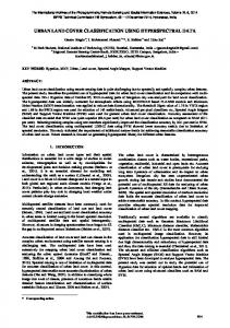
where 𝜀 is nonzero small constant and 𝑤 is the weight of neuron. The setting of 𝜀 ensures that inactive neurons receive a nonzero gradient value, so that the neuron has the possibility of being activated. Based on the above analysis, a deep network framework for hyperspectral data classification based on deep convolutional neural network is proposed in Figure 1. In the proposed deep CNN model, the first layer, the third layer, and the fifth layer are convolution layers, which realized feature extraction from lower level to higher level. The second layer, the fourth layer, and the sixth layer are lower sampling layers, used for feature dimension reduction. The final layer is the output layer which is whole connection layer and output of the final extraction features.

3. Structure Design of Hyperspectral Data Classification Framework

4. Exponential Momentum Gradient Descent Algorithm

In deep convolutional neural network, input data, convolution kernel, and threshold parameter are the three most important issues [27–29]. The input data is the basis of

4.1. Error Transfer. Error transmission descends by two steps through forward propagation and reverse gradient, to conduct weight generation and adjustment. Using gradient

Journal of Sensors

3

x(1) x(2) .. .

x(n)

K(Xp , X1 ) K(Xp , X2 ) .. .

Output Y

K(Xp , Xn ) Original data

CNN

SVM

Figure 1: Classification framework based on EM-CNN.

descent method to update weight is shown in formula (2), and bias updating method is shown in formula (3) [30]: 𝑙 𝑙 = 𝑤old + 𝜂 (− 𝑤new

𝑙 𝑙 𝑏new = 𝑏old + 𝜂 (−

𝜕𝐸 ), 𝑙 𝜕𝑤old

𝜕𝐸 ). 𝑙 𝜕𝑏old

(2)

(3)

𝑙 −𝜕𝐸/𝜕𝑤old

is the In the formula, 𝜂 is the learning rate, 𝑙 is the gradient of gradient of error to weight, and −𝜕𝐸/𝜕𝑏old error to bias, namely, the sensitivity of parameter adjustment. In order to achieve weight and bias optimizing, the gradient of error to weight and the gradient of error to bias must be first obtained. For convolution layer, its output is shown as the following formula: 𝑥𝑗𝑙 = 𝑓 ( ∑ 𝑀𝑗 ∗ 𝐾𝑖𝑗𝑙 + 𝑏𝑗 ) ,

(4)

𝑖∈𝑀𝑗

where 𝑏𝑗 is the bias of 𝑗th type of feature diagram, 𝑀𝑗 is the block of input feature diagram, and 𝐾𝑖𝑗𝑙 is convolution kernel. According to derivation formula of sensitivity function, the sensitivity of convolution layer can be represented by the following formula: 𝛿𝑗𝑙

=

𝛽𝑗𝑙+1 up (𝛿𝑗𝑙+1 )

󸀠

𝑙

∘ 𝑓 (𝑢 ) ,

(5)

where 𝛽𝑗𝑙+1 is the convolution kernel of 𝑙 + 1 sampling layer,

up represents upper sampling, and 𝛿𝑗𝑙+1 is 1/4 of 𝛿𝑗𝑙 , so upper sampling should be conducted. ∘ symbol represents the multiplication of corresponding elements. Thus, the gradient of convolution layer error to bias is shown in formula (6). In the formula, (𝑢, V) is the element location of sensitivity matrix: 𝜕𝐸 𝜕𝐸 = = ∑ (𝛿𝑙 ) . 𝑙 𝜕𝑏𝑗 (𝑢,V) 𝑗 𝑢V 𝜕𝑏old

Substitute formula (5), (6) into formula (1), (2) and obtain the updated value of convolution layer’s weight. The output of sampling layer’s neural network can be expressed by formula (8), in which 𝛽𝑗𝑙 and 𝑏𝑗𝑙 , respectively, represent multiplicative bias and additive bias. Multiplicative bias is generally set as 1:

(6)

The gradient of convolution layer error to weight is shown in formula (7). In the formula, 𝑝𝑖𝑙−1 is the convolution block of 𝑥𝑖𝑙−1 and convolution kernel 𝐾𝑖𝑗 , (𝑢, V) is the element location of the block: 𝜕𝐸 𝜕𝐸 = = ∑ (𝛿𝑗𝑙 ) (𝑝𝑖𝑙−1 )𝑢V . (7) 𝑙 𝑢V 𝜕𝑤old 𝜕𝐾𝑖𝑗𝑙 (𝑢,V)

𝑥𝑗𝑙 = 𝑓 (𝛽𝑗𝑙 down (𝑥𝑗𝑙−1 ) + 𝑏𝑗𝑙 ) .

(8)

According to the sensitivity of calculating formula of gradient descent, the sensitivity of sampling layer obtained is shown as the following formula: 𝛿𝑗𝑙 = 𝛿𝑗𝑙+1 𝑤𝑗𝑙+1 ∘ 𝑓󸀠 (𝑢𝑙 ) .

(9)

Whereby the bias updating formula of sampling layer can be obtained, as is shown in formula (10). According to formula (3), bias value updating can be obtained: 𝜕𝐸 𝜕𝐸 = = ∑ (𝛿𝑙 ) . 𝑙 𝜕𝑏𝑗 (𝑢,V) 𝑗 𝑢V 𝜕𝑏old

(10)

4.2. Exponential Momentum Training Algorithm. The traditional gradient descent method only transmits gradient error between single layers, which lead to slow convergence rate of the network. Increasing the learning rate 𝜂 is a good way to improve the convergence speed. But it not only improves the convergence speed but also causes unstable problem of the network, namely, “oscillation.” Faced with this situation, paper [19] proposes the momentum method, which increases the convergence speed by adding momentum factor. Paper [31] proposes the self-adaptive momentum method based on paper [19]. However, neither of these methods considers the relation between oscillation, convergence, and momentum. And the momentum factor does not promote convergence and enhance learning performance. This paper applies error exponential function of gradient to adjust the pace of momentum factor. The function can increase the momentum factor at the flat region, which can accelerate the network convergence speed and can decrease the momentum factor at the steep region of error curve, which can avoid excessive network convergence. Such method can improve the convergence rate of the algorithm

4

Journal of Sensors

Alfalfa Corn-notill Corn-min Corn Grass/pasture Grass/trees Grass/pasture-mowed Hay-windrowed

Oats Soybeans-notill Soybeans-min Soybean-clean Wheat Woods Bldg-grass-tree-drives Stone-steel towers

Figure 2: Indian Pines hyperspectral imagery and ground truth of classification.

and avoid oscillation of convergence process. The updating formula of momentum factor is the following formula:

Class code

𝐷𝑘

󵄩 󵄩 , 𝑎 = exp (−𝜆 1 󵄩󵄩󵄩𝐷𝑘 󵄩󵄩󵄩 − 𝜆 2 ) 󵄩 󵄩󵄩Δ𝑤𝑘−1 󵄩󵄩󵄩2 󵄩 󵄩 𝐷𝑘 = −

𝜕𝐸 . 𝜕𝑤 (𝑘)

Table 1: Sixteen classes of Indian Pines dataset.

(11)

In the formula, Δ𝑤𝑘 = 𝑤𝑘+1 − 𝑤𝑘 , and 𝐷𝑘 represents the gradient of error to weight.

5. Experiment and Analysis In this section, the performance of the proposed algorithm is evaluated on AVIRIS and ROSIS hyperspectral dataset. The overall accuracy, generalized accuracy, and kappa parameters, the most three important criteria, are used to evaluate the performance of the proposed framework. 5.1. Data Description. In our experiments, we experimented and validated the proposed framework with AVIRIS and ROSIS hyperspectral datasets. AVIRIS hyperspectral data 92AV3C was obtained by the AVIRIS sensor in June 1992. ROSIS hyperspectral datasets were gathered by a sensor known as the reflective optics system imaging spectrometer (ROSIS-3) over the city of Pavia, Italy. In particular, we employed the Indian Pines dataset, which depicts Indiana and consists of 145 × 145 data size and 224 spectral bands in the wavelength range 0.4 to 2.510−6 meters. It contains a total of 16 categories, as shown in Table 1. Its true mark is shown in Figure 2. The other datasets we employed are the Pavia

C1 C2 C3 C4 C5 C6 C7 C8 C9 C10 C11 C12 C13 C14 C15 C16

Ground object class

Number of training samples

Number of testing samples

Alfalfa Corn-notill Corn-min Corn Grass/Pasture Grass/Trees Grass/pasture-mowed Hay-windrowed Oats Soybeans-notill Soybeans-min Soybean-clean Wheat Woods Bldg-Grass-Tree-Drives Stone-steel towers

30 734 434 134 297 397 16 289 10 538 1268 314 112 694 190 50

24 700 400 100 200 300 10 200 10 430 1200 300 100 600 190 45

University datasets, whose number of spectral bands are 102. Nine land cover classes are selected, which are shown in Figure 3. The numbers of samples for each class are displayed in Table 2. For investigating the performance of the proposed methods, experiments were organized step by step. The influence of the convolution kernel size and the depth of the network

Journal of Sensors

5 Table 2: Nine classes of Pavia dataset. Class code

Ground object class

Number of training samples

Number of testing samples

Alfalfa

30

24

C1

Asphalt Bare soil Bitumen Gravel Meadow

Metal sheets Bricks Shadow Trees

Figure 3: Pavia hyperspectral imagery and ground truth of classification.

on the classification results was first analyzed. Then, we verified the performance of exponential momentum training algorithm. Finally, classifications based on CNN framework were conducted. 5.2. Effect of Kernel Size and Depth. The influence of the kernel size and the network depth on the classification performance of the proposed framework is analyzed in this section. The deep convolution neural network is trained by a series of different kernel size and network depth under fixed network structure and algorithm parameters. The results are shown in Tables 3 and 4. Table 3 suggested that the convolution kernel size is less affected by the overall accuracy of the method, and it better be consistent with the features size of the image data. Table 4 results shows that the deeper structures can get better classification accuracy. 5.3. Exponential Momentum Training Algorithm. In this section, we verified the general accuracy and the convergence speed of the algorithm. We select adaptive momentum [31] and elastic momentum [32] as the comparative method to observe the iteration round change of loss function of training objectives. It can be easily seen from Figure 4 that the convergence point of adaptive momentum is 14, the convergence point of elastic momentum is 8, and the convergence point of exponential momentum is 7. So the convergence of iteration times of exponential momentum is the minimum, and its consumption of the training time is also the minimum. For the general accuracy test experiment, the LeNet5 neural network [33] and standard multiple neural network [34] are chosen for comparison. The accuracy results obtained are shown in Table 5. It can be seen from the table that, compared with the corresponding training models of the

C2

Bare soil

734

700

C3

Bitumen

434

400

C4

Gravel

134

100

C5

Meadows

297

200

C6

Metal sheets

397

300

C7

Bricks

16

10

C8

Shadow

289

200

C9

Trees

10

10

Table 3: Accuracy comparison of different kernel size. Kernel size Accuracy

3 35.2

7 95.2

9 98.7

11 98.2

15 90.5

17 50.2

Table 4: Accuracy comparison of different depth. Depth Accuracy

3

4

5

6

7

9

40.5

85.3

89.5

94.5

98.8

99.6

Table 5: Accuracy comparison of algorithms’ image recognition. Momentum method

EFM-CNN network

LeNet5 neural network

Multiple neural network

Exponential momentum

98.69

98.24

73.03

97.65

97.5

72.5

97.10

97.00

65.50

Elastic momentum Adaptive momentum

standard momentum and adaptive momentum, the exponential momentum training method can elevate the classification accuracy on different network. 5.4. Comparing with Other Methods 5.4.1. Comparing with Other Feature Extraction Methods. We verify the effectiveness of the proposed feature extraction method from the sense of classification, by comparing our algorithm with other classical feature extraction methods, involving principle component analysis- (PCA-) SVM, kernel PCA- (KPCA-) logistic regression (LR), independent component analysis- (ICA-) SVM, nonnegative matrix factorization- (NMF-) LR, and factor analysis- (FA-) SVM.

6

Journal of Sensors Table 6: Accuracy comparison of different classifier.

Datasets

Measurements

Pavia

Indian

SAE-LR

RBP-SVM

PCA-RBP-SVM

Joint

Spatial

Joint

Spatial

Joint

Spatial

Joint

Overall accuracy

0.9514

0.9852

0.9455

0.9845

0.9625

0.9869

0.9448

0.9791

average accuracy Kappa coefficient

0.9401 0.9358

0.9732 0.9850

0.9370 0.9289

0.9711 0.9794

0.9522 0.9431

0.9790 0.9859

0.9281 0.9246

0.9689 0.9758

Overall accuracy average accuracy Kappa coefficient

0.9589 0.9475 0.9594

0.9735 0.9669 0.9750

0.9564 0.9412 0.9539

0.9722 0.9615 0.9439

0.9653 0.9517 0.9605

0.9876 0.9795 0.9862

0.9514 0.9375 0.9547

0.9701 0.9599 0.9418

0.10

1.00

0.09

0.95

0.08

0.90

0.07 0.06

Accuracy

Mean square error

EFM-CNN-SVM

Spatial

0.05 0.04 0.03

0.85 0.80 0.75 0.70

0.02 0.65

0.01 0.00

0

1000 2000 3000 4000 5000 6000 7000 8000 9000 10000 Train degrees Traingdx Traingdfm

Proposed

Figure 4: Convergence curve.

All the logistic regression classifiers are set to have learning rate 0.1 and are iterated on the training data for 8000 epochs. The result is shown in Figure 5. Experiments show that, by combining with SVM, the proposed method outperforms all other feature extraction methods and gets the highest accuracy. 5.4.2. Comparing with Other Classification Methods. We examine the classification accuracy of EFM-CNN-SVM framework by comparing proposed framework with spatialdominated methods, such as radial basis function- (RBF-) linear SVM, principle component analysis- (PCA-) RBFSVM, and stacked autoencoder- (SAE-) logistic regression (LR). By putting both the spectral and spatial information together to form a hybrid input and utilizing the deep classification framework detailed in Section 3, we get the highest classification accuracy we have ever attained. The experiments were performed with same parameter settings above 100. The results are shown in Table 6 and Figure 6. From Table 6, we can see that the EFM-CNN-SVM method turns out to be better on all other methods. And the joint features yield higher accuracy than spectral features in terms of mean performance. In Figure 6, we look into the classification accuracy from a visual perspective. It can be seen that

0.60 1.0

1.5

2.0 2.5 3.0 3.5 4.0 Number of extracted features (×20)

PCA-SVM KPCA-LR NMF-LR

4.5

5.0

FA-SVM The proposed

Figure 5: Comparison with other feature extraction methods.

classification results of proposed method are closest to the ideal classification results other than RBF-SVM and linear SVM methods.

6. Conclusion In this paper, a hyperspectral data classification framework is proposed based on deep CNN features extraction architecture. And an improved error transmission algorithm, selfadaptive exponential momentum algorithm, is proposed. Experiments results show that the improved error transmission algorithm converged quickly compared to homologous error optimization algorithm such as adaptive momentum and elastic momentum. And proposed EFM-CNN-SVM framework has been proven to provide better performance than PCA-SVM, KPCA-SVM, and SAE-LR frameworks. Our experimental results suggest that deeper layers always lead to higher classification accuracies, though operation time and accuracy are contradictory. It has shown that the deep architecture is useful for classification and the high-level spectral-spatial feature, increasing the classification accuracy. When the data scale is larger, the extracted feature has better recognition ability.

Journal of Sensors

7

Ideal

Proposed method

RBF-SVM

Linear SVM

Figure 6: Classification of Indian Pines dataset based on EFM-CNN-SVM.

Competing Interests The authors declare that they have no competing interests.

Acknowledgments This work is supported by the National 863 High Tech Research and Development Program (2010AA7080302).

References [1] F. M. Lacar, M. M. Lewis, and I. T. Grierson, “Use of hyperspectral imagery for mapping grape varieties in the Barossa Valley, South Australia,” in Proceedings of the 2001 International Geoscience and Remote Sensing Symposium (IGARSS ’01), pp. 2875–2877, IEEE, Sydney, Australia, July 2001. [2] P. W. T. Yuen and M. Richardson, “An introduction to hyperspectral imaging and its application for security, surveillance and target acquisition,” Imaging Science Journal, vol. 58, no. 5, pp. 241–253, 2010. [3] T. J. Malthus and P. J. Mumby, “Remote sensing of the coastal zone: an overview and priorities for future research,” International Journal of Remote Sensing, vol. 24, no. 13, pp. 2805–2815, 2003. [4] J. M. Bioucas-Dias, A. Plaza, G. Camps-Valls, P. Scheunders, N. Nasrabadi, and J. Chanussot, “Hyperspectral remote sensing data analysis and future challenges,” IEEE Geoscience & Remote Sensing Magazine, vol. 1, no. 2, pp. 6–36, 2013. [5] M. T. Eismann, A. D. Stocker, and N. M. Nasrabadi, “Automated hyperspectral cueing for civilian search and rescue,” Proceedings of the IEEE, vol. 97, no. 6, pp. 1031–1055, 2009. [6] E. K. Hege, W. Johnson, S. Basty et al., “Hyperspectral imaging for astronomy and space surviellance,” in Imaging Spectrometry IX, vol. 5159 of Proceedings of SPIE, pp. 380–391, January 2004. [7] F. V. D. Meer, “Analysis of spectral absorption features in hyperspectral imagery,” International Journal of Applied Earth Observation & Geoinformation, vol. 5, no. 1, pp. 55–68, 2004. [8] S. Rajan, J. Ghosh, and M. M. Crawford, “An active learning approach to hyperspectral data classification,” IEEE Transactions on Geoscience and Remote Sensing, vol. 46, no. 4, pp. 1231– 1242, 2008. [9] Q. L¨u and M. Tang, “Detection of hidden bruise on kiwi fruit using hyperspectral imaging and parallelepiped classification,” Procedia Environmental Sciences, vol. 12, no. 4, pp. 1172–1179, 2012.

[10] G. M. Foody and A. Mathur, “A relative evaluation of multiclass image classification by support vector machines,” IEEE Transactions on Geoscience & Remote Sensing, vol. 42, no. 6, pp. 1335– 1343, 2004. [11] Y. Chen, X. Zhao, and X. Jia, “Spectral-spatial classification of hyperspectral data based on deep belief network,” IEEE Journal of Selected Topics in Applied Earth Observations & Remote Sensing, vol. 8, no. 6, pp. 2381–2392, 2015. [12] Y. Chen, Z. Lin, X. Zhao, G. Wang, and Y. Gu, “Deep learningbased classification of hyperspectral data,” IEEE Journal of Selected Topics in Applied Earth Observations & Remote Sensing, vol. 7, no. 6, pp. 2094–2107, 2014. [13] A. Krizhevsky, I. Sutskever, and G. E. Hinton, “Imagenet classification with deep convolutional neural networks,” in Proceedings of the 26th Annual Conference on Neural Information Processing Systems (NIPS ’12), pp. 1097–1105, Lake Tahoe, Nev, USA, December 2012. [14] G. E. Hinton and R. R. Salakhutdinov, “Reducing the dimensionality of data with neural networks,” Science, vol. 313, no. 5786, pp. 504–507, 2006. [15] Z. Zhu, C. E. Woodcock, J. Rogan, and J. Kellndorfer, “Assessment of spectral, polarimetric, temporal, and spatial dimensions for urban and peri-urban land cover classification using Landsat and SAR data,” Remote Sensing of Environment, vol. 117, pp. 72–82, 2012. [16] D. Yu, L. Deng, and S. Wang, “Learning in the deep structured conditional random fields,” in Proceedings of the Neural Information Processing Systems Workshop, pp. 1–8, Vancouver, Canada, December 2009. [17] A.-R. Mohamed, T. N. Sainath, G. Dahl, B. Ramabhadran, G. E. Hinton, and M. A. Picheny, “Deep belief networks using discriminative features for phone recognition,” in Proceedings of the 36th IEEE International Conference on Acoustics, Speech, and Signal Processing (ICASSP ’11), pp. 5060–5063, Prague, Czech Republic, May 2011. [18] B. H. M. Sadeghi, “A BP-neural network predictor model for plastic injection molding process,” Journal of Materials Processing Technology, vol. 103, no. 3, pp. 411–416, 2000. [19] P. Baldi and K. Hornik, “Neural networks and principal component analysis: learning from examples without local minima,” Neural Networks, vol. 2, no. 1, pp. 53–58, 1989. [20] Y. Bengio, P. Lamblin, D. Popovici, and H. Larochelle, “Greedy layer-wise training of deep networks,” in Proceedings of the 20th Annual Conference on Neural Information Processing Systems (NIPS ’06), pp. 153–160, Cambridge, Mass, USA, December 2006. [21] G. E. Hinton, “Apractical guide to training restricted Boltzmann machines,” Tech. Rep. UTML TR2010-003, Department of

8

[22]

[23]

[24]

[25]

[26]

[27]

[28]

[29]

[30]

[31]

[32]

[33]

[34]

Journal of Sensors Computer Science, University of Toronto, Toronto, Canada, 2010. R. Salakhutdinov and G. E. Hinton, “Deep Boltzmann machines,” in Proceedings of the International Conference on Artificial Intelligence and Statistics, pp. 448–455, Clearwater Beach, Fla, USA, April 2009. G. E. Hinton, S. Osindero, and Y.-W. Teh, “A fast learning algorithm for deep belief nets,” Neural Computation, vol. 18, no. 7, pp. 1527–1554, 2006. Y. Bengio, P. Lamblin, D. Popovici, and H. Larochelle, “Greedy layer-wise training of deep networks,” in Proceedings of the Neural Information Processing Systems, pp. 153–160, Cambridge, Mass, USA, 2007. M. D. Zeiler and R. Fergus, “Stochastic pooling for regularization of deep convolutional neural networks,” https://arxiv.org/ abs/1301.3557. H. Larochelle, D. Erhan, A. Courville, J. Bergstra, and Y. Bengio, “An empirical evaluation of deep architectures on problems with many factors of variation,” in Proceedings of the 24th International Conference on Machine Learning (ICML ’07), pp. 473–480, Corvallis, Ore, USA, June 2007. Y. Bengio, G. Guyon, V. Dror et al., “Deep learning of representations for unsupervised and transfer learning,” in Proceedings of the Workshop on Unsupervised & Transfer Learning, Bellevue, Wash, USA, July 2011. Y. Bengio, A. Courville, and P. Vincent, “Representation learning: a review and new perspectives,” IEEE Transactions on Pattern Analysis & Machine Intelligence, vol. 35, no. 8, pp. 1798– 1828, 2013. W. Ouyang and X. Wang, “Joint deep learning for pedestrian detection,” in Proceedings of the 14th IEEE International Conference on Computer Vision (ICCV ’13), pp. 2056–2063, December 2013. N. B. Karayiannis, “Reformulated radial basis neural networks trained by gradient descent,” IEEE Transactions on Neural Networks, vol. 10, no. 3, pp. 657–671, 1999. S. S. Agrawal and V. Yadava, “Modeling and prediction of material removal rate and surface roughness in surface-electrical discharge diamond grinding process of metal matrix composites,” Materials and Manufacturing Processes, vol. 28, no. 4, pp. 381– 389, 2013. W. Tan, C. Zhao, H. Wu, and R. Gao, “A deep learning network for recognizing fruit pathologic images based on flexible momentum,” Nongye Jixie Xuebao/Transactions of the Chinese Society for Agricultural Machinery, vol. 46, no. 1, pp. 20– 25, 2015. N. Yu, P. Jiao, and Y. Zheng, “Handwritten digits recognition base on improved LeNet5,” in Proceedings of the 27th Chinese Control and Decision Conference (CCDC ’15), pp. 4871–4875, May 2015. D. Shukla, D. M. Dawson, and F. W. Paul, “Multiple neuralnetwork,” IEEE Transactions on Neural Networks, vol. 10, no. 6, pp. 1494–1501, 1999.

International Journal of

Rotating Machinery

Engineering Journal of

Hindawi Publishing Corporation http://www.hindawi.com

Volume 2014

The Scientific World Journal Hindawi Publishing Corporation http://www.hindawi.com

Volume 2014


Distributed Sensor Networks

Journal of

Sensors Hindawi Publishing Corporation http://www.hindawi.com

Volume 2014


Volume 2014


Volume 2014

Journal of

Control Science and Engineering

Advances in

Civil Engineering Hindawi Publishing Corporation http://www.hindawi.com


Volume 2014

Volume 2014

Submit your manuscripts at http://www.hindawi.com Journal of

Journal of

Electrical and Computer Engineering

Robotics Hindawi Publishing Corporation http://www.hindawi.com


Volume 2014

Volume 2014

VLSI Design Advances in OptoElectronics


Navigation and Observation Hindawi Publishing Corporation http://www.hindawi.com

Volume 2014



Chemical Engineering Hindawi Publishing Corporation http://www.hindawi.com

Volume 2014

Volume 2014

Active and Passive Electronic Components

Antennas and Propagation Hindawi Publishing Corporation http://www.hindawi.com

Aerospace Engineering


Volume 2014


Volume 2014

Volume 2014




Modelling & Simulation in Engineering

Volume 2014


Volume 2014

Shock and Vibration Hindawi Publishing Corporation http://www.hindawi.com

Volume 2014

Advances in

Acoustics and Vibration Hindawi Publishing Corporation http://www.hindawi.com

Volume 2014