Deep Learning in Big Image Data: Histology Image

Accepted for Int. Conference on BIG DATA and Advanced Analytics, Minsk, Belarus, 15-17 June, 2016

Deep Learning in Big Image Data: Histology Image Classification for Breast Cancer Diagnosis V.A. Kovalev, A.A. Kalinovsky, V.A. Liauchuk Biomedical Image Analysis Department United Institute of Informatics Problems National Academy of Sciences of Belarus [email protected] This paper present results of the use of Deep Learning approach and Convolutional Neural Networks (CNN) for the problem of breast cancer diagnosis. Specifically, the main goal of this particular study was to detect and to segment (i.e. delineate) regions of micro- and macro-metastases in whole-slide images of lymph node sections. The whole-slide imaging of tissue probes produces very large histological images. The size of resultant color RGB images typically ranges between 50 000х50 000 and 200 000x200 000 pixels and they considered as a basic component of computerized methods in recent Digital Pathology. Original hematoxylin and eosin stained wholeslide images produced by two different optical microscope scanners were kindly provided by founders of CAMELYON16 world-wide competition [1]. A total of 0.6 million of square-shaped “image tiles” of 256х256 pixels in size (300 000 image tiles for each scanner type) were sub-sampled from original images for creating two training sets. These image sets were used for training of two respective Convolutional Networks. The training was performed based on Caffe CNN framework, which has been ran on a personal computer with recent i7 Intel CPU and an additional GPU of Nvidia TITAN X type equipped with 3072 CUDA Cores and 12 Gb of GDDR5 onboard memory. At the segmentation stage, the two trained Convolutional Networks were used for categorization of every image tile of each whole-slide test image to either tumor or non-tumor class using the sliding window technique. As a result, it was demonstrated that the Deep Learning approach and Convolutional Networks provide high classification accuracy, which allows harnessing them for segmentation of whole-slide Digital Pathology images by way of region-based classification.

Digital Pathology as the source of Big Medical Image Data The histopathology image analysis based on light microscopy has long been recognized as a gold standard in cancer diagnosis. However, recently it is commonly realized that one of the biggest challenges for pathologists is managing the huge amounts of data which are generated by modern microscope scanners daily [2, 3] As stated by Dr. Wenyi Luo and Prof. Lewis Hassell from Department of Pathology, University of Oklahoma Health Center [2], although glass slides provide highly efficient ways to convey information needed to make the initial diagnoses, they are often inefficient, expensive, and time-consuming when it comes to physical management, consultation, education, and research. Modern Digital Pathology provides more efficient and cost-effective means of presenting, transmitting, archiving and transporting pathology image data. The whole slide imaging is now the primary means of pathology image capture, store, and evaluation which used for both diagnostic [2-4] and education (e.g [5]) purposes. A number of use cases presented in [2] demonstrate a variety of ways that Digital Pathology can be used to facilitate pathology practice and education. The whole-slide imaging of tissue probes produces very large color histological images the size of which typically ranges between 50 000х50 000 and 200 000x200 000 pixels. As a consequence, such large image size induces various problems of different kinds which can be conditionally subdivided into technical and methodological ones. Although purely technical problems of image store, retrieval and visualization can be resolved using advanced computing facilities, the expert visual examination of such huge and content-rich images by pathologists becomes not feasible in many occasions. Thus, the availability and permanent spreading of high resolution whole-slide images has reinforced the interest of the medical image analysis community to the computerized methods and corresponding software. This is resulted in increasing number of research and development works as well as in the growing number of publications in the field.

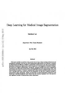
Since the majority of image analysis tasks in field of digital pathology are essentially of the image classification type, combining the novel Big Data, Deep Learning with Convolutional Neural Networks approaches appears to be very promising. The purpose, applied tasks and main goals This paper presents results of the use of Deep Learning approach for automation of histology image analysis in the problem of breast cancer diagnosis. These results were obtained by authors during participation in open world-wide CAMELYON16 competition [1]. The challenge was focused on the detection of micro- and macro-metastases in lymph node images. According to the competition founders, this subject is highly relevant to many practical cases because the lymph node metastases occur in most cancer types (e.g. breast, prostate, colon). The lymph nodes in the underarm are the first place breast cancer is likely to spread. Metastatic involvement of lymph nodes is one of the most important prognostic variables in breast cancer. Prognosis is poorer when cancer has spread to the lymph nodes. The diagnostic procedure for pathologists is, however, tedious, time-consuming and prone to misinterpretation [1]. In the context of modern machine leaning methods and software tools the primary goal of this study was to examine the ability of recently introduced Convolutional Networks as one of the most intriguing image-related Deep Learning tools on the hard problem of automatic detection and segmentation of metastases in whole-slide images of lymph node sections. Materials and Methods General Notes. Due to certain color differences easily observed in slide images produced by two different scanners involved in the experimentation (see Fig. 1) they were analyzed and segmented in exactly the same way but in totally separate runs.

Fig. 1. Examples of original whole-slide images acquired with the help of a 3DHistech (top panel) and Hamamatsu NDPI (bottom panel) light microscope scanners.

The segmentation method followed in this study was based on the sliding window technique. At each window position the underlying small image region was categorized with certain probability either to the tumor or non-tumor class. Categorization (class prediction) was performed using neural networks which were trained prior to the segmentation procedure on suitable set of small, square-shaped image patches (image “tiles”). Original Images. Whole-slide images are generally stored in a multi-resolution pyramid structure [6]. Image files contain multiple downsampled versions of the original image. The highest resolution provided on the Level 0. Each image in the pyramid is stored as a series of tiles, to facilitate rapid retrieval of subregions of the image. Reading these images using standard image tools or libraries is a challenge because these tools are typically designed for images that can comfortably be uncompressed into RAM or a swap file. OpenSlide [7] is a C library that provides a simple interface to read whole-slide images of different formats. A total of 340 original whole-slide images amounting for about 0.6 Terabyte of image data were used as an input for computational experiments being performed (see low resolution image examples of two scanner types depicted in Fig.1 above). They included 100 images (~171 GB) of normal tissue and 110 images (~216 GB) of tumor tissue samples affected by metastases. Both image sets have been used as a source for CNN training. Other 130 whole-slide images were allocated for testing of trained networks. It should be noted that the above mentioned 110 images acquired from tissue samples with metastasis not necessarily fully occupied by a tumor. Rather opposite, some of them contain only a tiny tumor invasion what makes the tumor detection and segmentation task very challenging. Fig. 2 illustrates a clear-cut case of original image regions where metastases bordering with normal tissue being sampled from a lymph node. It should be noted that the lucky cases like the one depicted in Fig. 2 are rare in real practice. More common cases of image regions, some of which falls into the category of hard-to-distinguish, are illustrated in figures that follow.

Fig. 2. Example image presenting a case with distinct border between the normal tissue region (upper part) and region affected by metastasis (underneath). The border depicted in dark-blue was drawn by a pathologist.

Image Training Sets. A total of 0.6 million of image tiles, i.e. square-shaped image patches were sampled from original slide images and used as training sets for two different networks corresponding to two types of whole-slide scanners. The tile size was set to 256x256 pixels as a compromise between the intention of tiles to be as small as possible for more accurate tumor border segmentation whereas be large enough to represent image semantics, i.e. contain sufficient quantity of characteristic morphological elements. The sampling was done by way of

moving 256x256 sampling window with the half-window step of 128 pixels over corresponding whole-slide image. Regions of interest included images of normal tissue and areas affected by metastasis. The later were annotated in a training set (i.e., segmented manually) by pathologists from Radboud University Medical Center (Nijmegen, the Netherlands) and from the University Medical Center Utrecht (Utrecht, the Netherlands). All the annotations were performed with the help of Automated Slide Analysis Platform (ASAP), which is an open source platform for visualizing, annotating and automatically analyzing whole-slide histopathology images. ASAP is built on top of several well-developed open source packages like OpenSlide, Qt and OpenCV and it can be downloaded from Github [8]. The sampling was done on the Level 0 with highest spatial resolution, separately for 3DHistech (Training Set-1) and Hamamatsu NDPI (Training Set-2) scanners. A brief description of training sets and typical image tile examples are presented in Tab. 1. The resultant sets of image tiles were shuffled at random and the necessary number of them moved into corresponding training sets. Tab. 1. Image training sets Class 1 Training “Tumor” Set-1 300 000 Class 2 image “Nontiles Tumor” Class 1 Training “Tumor” Set-2 300 000 image Class 2 tiles “NonTumor”

150 000 tiles sampled from metastasis regions annotated by pathologists as Group “_0”. 150 000 tiles sampled from regions conditionally called as norm, background, bubbles, erythrocytes, and epithelium. 150 000 tiles. Same types of regions as in Class 1 of Training Set-1. 150 000 tiles. Same types of regions as in Class 2 of Training Set-1.

It should be noted that despite the tissue regions affected by tumor holding some characteristic colorimetric and morphological features, which allow their correct classification, certain fraction of them appear very similar to the normal ones. Such regions can be almost impossible to differentiate for both pathology experts and machine learning methods. Examples of such regions are provided in Fig. 3. Training Convolutional Neural Networks. The two neural networks were trained using Nvidia Deep Learning GPU Training System (DIGITS) interface. DIGITS integrates the popular Caffe deep learning framework from the Berkeley Learning and Vision Center, and supports GPU acceleration using cuDNN to massively reduce training time [9]. The training was performed on a personal computer equipped with recent i7 Intel central processor and an additional GPU of Nvidia TITAN X type with 3072 CUDA Cores and 12 GB of GDDR5 onboard memory. The network training parameters were set to the following values:  Batch size: 64 (the minimum batch size to place network in GPU memory),  Solver: SGD Caffe solver,  Number of iterations: ~100000,  Number of epochs: 30,  Network architecture: GoogleNet [10].

Slide Image Segmentation by Classification of Patches. The classification algorithm employs neural network trained at the previous stage for categorization of every underlying 256x256 image patch at each sliding window position either to Tumor (i.e., metastasis) or to Non-Tumor class.

Fig. 3. Example image tiles of normal tissue (top panel) and metastasis (bottom panel) which are difficult to distinguish.

The process resulted in a probability map which represents the probability of belonging of each particular image locality to the class of metastasis. Each pixel of the map corresponds to a 256x256 region of original whole-slide image on the Level 0. Thus, each dimension of the map was 256 times smaller than the original high resolution whole slide image being considered on the Level 0 of pyramid. Post-Processing. The goal of post-processing stage was to extract coordinates and probability scores of possible lesion regions presented on a high-resolution histology image. Probability maps at the level 9 of pyramid obtained at the image classification stage were used here as input data. The post-processing stage consists of five major steps: Step-1: Converting the tumor probability map into the binary tumor map by way of thresholding using a minimum probability level MINPROB as a control parameter. Step-2: Extracting connected components of the binary tumor map.

Step-3: Removing connected components whose size is too small to be an invasion using MINSIZE control parameter. Step-4: Computing the tumor probability score PTUM, i.e. the probability that the extracted region as a whole belongs to the tumor class. After certain trials-and-error experiments, it was found that probability PTUM may be assumed to be 1 when the region exceeds certain MAXSIZE value and may be approximated by SIZE/MAXSIZE otherwise that is:

1 SIZE  MAX SIZE , . PTUM   SIZE  MAX SIZE , SIZE MAX SIZE Step-5: Defining coordinates of the extracted tumor region. Since the extracted region may have a complicated shape its coordinates may not be defined simply as center of its bounding box or center of gravity. This is because in both occasions the center may lie outside of detected region. Instead, in order to describe the reference point to possible lesion location we used coordinates of a point on the skeleton of the binary region, which is the closest to the center of gravity. Results Training of each of two neural networks took about 8 hours of time and approximately 11 GB of GPU memory. The potential discrimination ability of both networks was examined on the corresponding image subsets containing 300 000 image tiles each. Results are presented in Fig. 4 in form of ROC curves.

Fig. 4. ROC curves assessing the potential discrimination ability of two Convolutional Neural Networks trained for discrimination of metastatic regions in whole-slide scans obtained by two types of scanners. Note that the plot is enlarged towards top-left corner by factor of x10-3 in order to make the differences visible.

After completing the preliminary examination of neural networks, they were used for segmenting of the whole slide images by way of tile-wise recognition and categorization of every 256x256 region as well as calculating resultant tumor probability maps. Examples of output maps are given in Fig. 5. The probability maps of target images (see top row of Fig. 6) were converted into a binary image using threshold value MINPROB = 0.99. Results are presented at the bottom row of Fig. 6. Note that since the very high value of 0.99 of the probability is considered, both versions of maps appear almost as “binary” ones. Extracting connected components of the binary tumor maps was done using 8-connectivity condition. The MINSIZE control parameter which was employed for removing connected

components that unlikely to belong to the tumor class because they are too small was set to MINSIZE = 5 pixels.

Fig. 5. Examples of tumor regions manually labeled by pathology experts (green blobs) and corresponding tumor candidate regions obtained on the classification step with the help of convolutional neural networks (pink).

Fig. 6. Examples of tumor probability maps (top row) and their binary versions obtained with the threshold value MINPROB = 0.99 (bottom row). White contours presenting the tissue sample edges.

At the step of computing the tumor probability scores for the whole extracted region PTUM the most suitable MAXSIZE parameter was found to be MAXSIZE = 30 image pixels at the image pyramid Level 9. Fig. 7 provides examples of resultant tumor regions detected by the method by their reference locations given by color dots. The colors presenting probabilities of categorization of each region to the Tumor class in the color scale provided on the right.

Fig. 7. Examples of extracted reference points (colored dots) to the tumor regions detected by the method and colorcoded probabilities of categorization to the Tumor class. White contours presenting the tissue sample edges.

Finally, reference coordinates of location of each selected connected component were stored in the CSV files together with their probabilities. These CSV files were submitted to the competition. As a result, this study was ranked as winning the 13th position of the world competition on tumor localization [11]. The key intermediate results were also placed on a temporal, free access web site [12] to facilitate their in-depth check and to enable possible re-use. Conclusions The suggested method capitalizing on Deep Learning approach may be considered as a promising tool capable of an automatic identification and visualization of histological image structures relevant to the cancer patient conditions. References 1. 2.

http://camelyon16.grand-challenge.org/home/ Last visited 12 May 2016. Luo W., Hassell L.A. Use Cases for Digital Pathology. In: Digital Pathology: Historical Perspectives, Current Concepts and Future Applications, J.K. Kaplan, K.F.L. Rao (Eds), Springer International Publishing, ISBN 978-3-319-20378-2, 2016, pp. 5-15. 3. Beckwith B.A. Standards for Digital Pathology and Whole Slide Imaging. In: Digital Pathology: Historical Perspectives, Current Concepts and Future Applications, J.K. Kaplan, K.F.L. Rao (Eds), Springer International Publishing, ISBN 978-3-319-20378-2, 2016, pp. 87-97. 4. Eccher A., Neil D., Ciangherotti A., Cima L., et al. Digital reporting of whole-slide images is safe and suitable for assessing organ quality in preimplantation renal biopsies, Human Pathology, vol. 47, Issue 1, 2016, pp. 115-120. 5. Saco A., Bombi J.A., Garcia A., Ramírez J., Ordi J. Current Status of Whole-Slide Imaging in Education. Pathobiology, vol. 83, 2016, pp.79–88. 6. http://camelyon16.grand-challenge.org/data/ Last visited 12 May 2016. 7. http://openslide.org/ Last visited 12 May 2016. 8. https://github.com/GeertLitjens/ASAP Last visited 12 May 2016. 9. https://devblogs.nvidia.com/parallelforall/deep-learning-computer-vision-caffe-cudnn/ Last visited 12 May 2016. 10. Szegedy, Christian, et al. Going deeper with convolutions. Proceedings of the IEEE Conference on Computer Vision and Pattern Recognition, 2015, pp. 1-9. 11. http://camelyon16.grand-challenge.org/results/ Last visited 12 May 2016 (registration is necessary). 12. http://imlab.grid.by/camelyon2016/ Last visited 12 May 2016.