Deep Learning Methods for Underwater Target Feature Extraction and ...

Hindawi Computational Intelligence and Neuroscience Volume 2018, Article ID 1214301, 10 pages https://doi.org/10.1155/2018/1214301

Research Article Deep Learning Methods for Underwater Target Feature Extraction and Recognition Gang Hu ,1,2 Kejun Wang ,1 Yuan Peng,3 Mengran Qiu,3 Jianfei Shi,1 and Liangliang Liu1 1

College of Automation, Harbin Engineering University, Harbin 150001, China College of Business, Anshan Normal University, Anshan 114007, China 3 760 Research Institute of China Shipbuilding Industry, Liaoning, Anshan, China 2

Correspondence should be addressed to Kejun Wang; [email protected] Received 11 September 2017; Revised 9 December 2017; Accepted 15 January 2018; Published 27 March 2018 Academic Editor: Ras¸it K¨oker Copyright © 2018 Gang Hu et al. This is an open access article distributed under the Creative Commons Attribution License, which permits unrestricted use, distribution, and reproduction in any medium, provided the original work is properly cited. The classification and recognition technology of underwater acoustic signal were always an important research content in the field of underwater acoustic signal processing. Currently, wavelet transform, Hilbert-Huang transform, and Mel frequency cepstral coefficients are used as a method of underwater acoustic signal feature extraction. In this paper, a method for feature extraction and identification of underwater noise data based on CNN and ELM is proposed. An automatic feature extraction method of underwater acoustic signals is proposed using depth convolution network. An underwater target recognition classifier is based on extreme learning machine. Although convolution neural networks can execute both feature extraction and classification, their function mainly relies on a full connection layer, which is trained by gradient descent-based; the generalization ability is limited and suboptimal, so an extreme learning machine (ELM) was used in classification stage. Firstly, CNN learns deep and robust features, followed by the removing of the fully connected layers. Then ELM fed with the CNN features is used as the classifier to conduct an excellent classification. Experiments on the actual data set of civil ships obtained 93.04% recognition rate; compared to the traditional Mel frequency cepstral coefficients and Hilbert-Huang feature, recognition rate greatly improved.

1. Introduction Deep learning is a new area of machine learning research aimed at establishing a neural network that simulates human brain analysis and learning. The concept of deep learning was proposed by Hinton in 2006 [1]. In recent years, deep learning has drawn wide attention in the field of pattern analysis and has gradually become the mainstream method in the fields of image analysis and recognition and speech recognition [2]. In recent years, some people apply it to the speech signal denoising [3] and the dereverberation problem [4]. Convolutional Neural Network (CNN) is one of the core methods in depth learning theory. CNN can be classified as deep neural network (DNN) but belongs to supervised learning method. Y. LeCun proposed CNN is the first real multilayer structure learning algorithm, which uses space relative relationship to reduce the number of parameters to improve training performance, and has achieved success in

handwriting recognition. Professor Huang Guangbin from Nanyang Technological University first proposed extreme learning machine in 2004. Extreme learning machine (ELM) has been proposed for training single hidden layer feed forward neural networks (SLFNs). Compared to traditional FNN learning methods, ELM is remarkably efficient and tends to reach a global optimum. In this paper, CNN and ELM methods are introduced into underwater acoustic target classification and recognition, and a underwater target recognition method based on depth learning is proposed. In view of the prominent performance of convolutional neural network in speech recognition and its frequent usage in speech feature extraction, the convolutional neural network is used to extract the features of underwater ship’s sound signal, and the corresponding network model and parameter setting method are given. This method is compared with Support Vector Machine (SVM) [5] and k-nearest neighbors (KNN) [6], Hilbert-Huang Transform (HHT) [7], and Mel

2 frequency cepstral coefficients (MFCC) [8] methods. The experimental results show that underwater target recognition based on depth learning has a higher recognition rate than the traditional method. Then ELM fed with the CNN features is used as the classifier to conduct an excellent classification. Experiments on the actual data set of civil ships obtained 93.04% recognition rate; compared to the traditional Mel frequency cepstral coefficients and Hilbert-Huang feature, recognition rate greatly improved.

2. Related Work The current development of passive sonar high-precision underwater target automatic identification method to prevent all types of water targets in the raid is to strengthen the urgent task of the modern war system. A series of theoretical methods and technical means involved in the automatic identification of underwater targets can be applied not only to national defense equipment research but also to marine resources exploration, marine animal research, speech recognition, traffic noise recognition, machine fault diagnosis, and clinical medical diagnosis field. In the 1990s, researchers of all countries applied artificial neural network into underwater target recognition system. The methods such as power spectrum estimation, shorttime Fourier transform, wavelet transform, Hilbert-Huang transform, fractal, limit cycle, and chaos [8–11] failed to fully consider the structure features of sound signal and the features extracted by such methods have prominent problems, such as worse robustness and low recognition rate. In 2006, a paper published on Science, the world top level academic journal, by Geoffrey Hinton, machine learning master and professor of University of Toronto and his student Ruslan, aroused the development upsurge [12] of deep learning in research field and application field. Since then, many researchers began working on deep learning research. In 2009, Andrew Y. Ng, etc. [13] extracted once again the features of spectrogram by using convolutional deep belief networks, and all of the results derived from use of extracted features to multiple voice recognition tasks are superior to the ones of the system which recognizes by taking Mel frequency cepstrum coefficient directly as a feature. In 2011, Hinton used restricted Boltzmann machine [14] to learn the waveform of original voice signal to obtain the distinguishable advanced features. The experiment shows that such method is better than the traditional Mel frequency spectrum feature in performance. In 2012, four major international scientific research institutions summed up the progress made by deep learning in sound recognition task [15] and pointed out in the paper that the experiments show the effect of deep neural network is better than the one of traditional Gaussian mixed model. In 2013, Brian Kingsbury, researcher of IBM, and several other persons [16] took the logarithmic Mel filter coefficient as the input of deep convolution network and further extracted the “original” features (Mel filter coefficient), and the experiment shows that the recognition rate has a relative increase of 13–30% compared to the traditional Gaussian mixed model and has a relative increase of 4–12% compared to deep neural networks. The research of Palaz et

Computational Intelligence and Neuroscience al. [17] shows that the system of using original voice signal as the input of convolutional neural networks to estimate phoneme conditional probability has achieved similar or better results than the TIMIT phoneme recognition task of the standard hybrid type HMM/ANN system. In 2014, Palaz et al. [17] put forward the convolutional neural networks of restriction right sharing mechanism and once again achieved amazing results. In 2015, three artificial intelligent masters, LeCun et al. [18], jointly published an overview titled “deep learning” on Nature, giving a comprehensive introduction on the theory of deep learning. Nowadays, deep learning has become the research hot spot of the world. Considering the outstanding performance of convolutional neural networks in voice recognition, this article uses convolutional neural networks to conduct feature extraction and recognition to underwater ship voice signal.

3. Deep Convolutional Neural Networks Under the inspiration of the structure of visual system, Convolutional neural networks (CNN) are developed. The first convolutional neural networks calculation model is put forward in the neural recognizer of Fukushima, which applies the neuron with the same parameters to different positions of the upper layer of neural networks based on partial connection and hierarchical organization image transformation, thus generating a kind of translation invariant neural network structural form. Afterwards, based on such thought, AbdelHamid et al. [19] designed and trained convolutional neural network by using error gradient and demonstrate an outstanding performance in handwriting character recognition task. The convolutional neural networks can be regarded as kind of transformation of standard neural networks, which introduce a kind of so called convolutional layer and sampling layer structure rather than using the whole connection structure like the traditional neural networks. Deep convolutional neural networks refer to the networks containing two layers or more than two layers of convolutional layer and sampling layer in the whole network. Each convolutional layer contains several different convolvers (filters) and these convolvers make observation to all partial features of the signal. Next to convolutional layer usually comes sampling layer, and sampling layer reduces the input node numbers of next layer by making the sampling of fixed window length to the output node numbers of the convolutional layer so as to control the complexity of the model. Then, convolution and sampling are made again to the output features of sampling layer, thus forming a kind of layered feature extractor and output of each layer can be regarded as an advanced expression form (i.e., advanced feature) of the “original” voice signal. Though convolutional neural networks also can realize classification of signal, its classification effect mainly relies on the artificial neural networks classifier formed by whole connection layer, while the artificial neural networks classifier has the problems such as worse generalization ability and local optimum, so this article only makes feature extraction by using convolutional networks. The structure of feature extraction of the convolutional neural networks herein is shown in Figure 1.

Computational Intelligence and Neuroscience

3

Pooling Signal input

Pooling

Convolution

CNN feature Output

Convolution Convolution

64 Map

128 Map

3 neurons

2000 500 Map neurons

100

Figure 1: Structure chart of deep convolutional networks.

Different from Multilayer Perception (MLP) and other neural network structures, CNN introduces three important concepts: partial connection, pooling, and weight sharing. Hereunder, we will introduce in detail the CNN structure in sound recognition and how to understand such three important concepts of CNN in sound recognition. 3.1. Partial Connection and Weight Sharing. In traditional BP network, the neurons in each layer show a one-dimensional linear array structure, with neuron nodes between each layer fully connected, while, in convolutional neural networks, neurons of each layer no longer adopt full connection form, with neurons at lower layer connected partially with some neurons at upper layer (partial connection). Figures 2 and 3, respectively, represent fully connected neural networks and partially connected neural networks. As far as Figures 2 and 3 are concerned, the number of weights that need to be trained between fully connected neural network 𝑁 − 1 layer and 𝑁 layer is 24 (4 × 6) while the number of weights that need to be trained between partially connected neural networks 𝑁 − 1 layer and 𝑁 layer is only 12 (4 × 3). In this case, the number of training parameters only reduces slightly, but for a large neural network, each layer contains hundreds of neurons; the advantages of partial connection will become more prominent. Weight sharing mechanism can further reduce the number of parameters that need to be trained in the networks. As shown in Figure 3, is concerned, if the weight sharing mechanism is used, the four groups of weight in the figure are the same (with each group assigned 3 weights, i.e., the convolutional kernel as mentioned hereunder); then there are only three weights that need to be trained between layer 𝑁−1 and layer 𝑁, thus significantly reducing network parameters and reducing the complexity of the model. 3.2. Build the Input Features of Convolutional Networks. The most commonly used feature in sound recognition is Mel frequency cepstrum coefficient (MFCC), which is widely applied in semantic recognition and voice recognition; however its recognition rate is not ideal. In the course of extracting the features of MFCC, the feature extraction is

N + 1 layer

N layer

N − 1 layer

Figure 2: Sketch figure of full connection neural networks.

N + 1 layer

N layer

N − 1 layer

Figure 3: Sketch figure of partial connection.

made only according to experiences, not considering inner link of signals themselves. In order to rationally use all of the information of the signal and extract a more suitable feature, this article adopts the extraction method of extracting self-adaptively the advanced features of signal through multilayer convolution by taking the original sound signal after overlapping framing directly as the input feature figure of convolutional networks. The input feature sketch figure of convolutional networks is built in Figure 4. As is shown in Figure 4, firstly, the input sound signal is a one-dimensional signal. Different from traditional method,

4

Computational Intelligence and Neuroscience Convolutional kernel

Weight sharing

First Second Third frame frame frame

Number N frame

Input feature

Original Sound Signals

Convolutional layer output feature

Figure 4: Build the input features of convolutional networks.

Figure 5: Sketch figure of convolution process of single input feature figure.

this article causes the original sound signal to be processed directly by framing (framing method is overlapping segmentation, frame length is 170 ms, and frame shift is 10 ms), with each frame after framing as an input sample of convolutional networks, that is, as the input feature figure of deep convolutional networks. 3.3. Convolutional Layer. As the convolutional layer of convolutional neural networks has been defined with corresponding receptive field, for the signal of each neuron of convolutional layer, only those transmitted from their receptive field can be accepted. Each neuron in convolutional layer is only partially connected to input of current layer, which is equivalent to using a convolutional kernel to perform ergodic convolution to the input feature figure of current layer. Moreover, as one kind of convolutional kernel can only observe limited information, in practical application, multiple different convolvers are usually used to observe from different perspectives so as to acquire more amount of information. In convolutional layer, the following two circumstances may occur: one is that there is only one input feature figure of convolutional layer; another is there are many input feature figures of convolutional layer. Given the above different circumstances, in order to make a better explanation, this article performs a detailed argumentation by combining the figures and texts. As is shown in Figure 5, there is only one input feature figure of convolutional layer (the process from input layer to convolutional layer), where the value of convolution result coming from the convolution to certain part of the feature figure by convolutional kernel and output by nonlinear function is the activated value of corresponding neuron in the feature figure of convolutional layer, and a convolutional layer output feature figure can be acquired by traversal input feature figure with convolutional kernel, and such output feature figure is equivalent to another kind of expression form to upper layer of input feature, that is, a feature learnt through convolutional neural networks. Many feature figures can be

acquired from convolutional layer by traversal input feature figure with multiple convolutional kernels, by which, signals with different features can be extracted (different connection lines in the figure represent the connection of different convolutional kernels). The size and number of the convolutional kernels have an important impact on the performance of the whole network, and the key of deep convolutional networks is to learn the contents, size, and number of convolutional kernels and determine an appropriate convolutional kernel for adaptive feature extraction through learning mass data. If the input of convolutional layer has only one feature figure, the output of each neuron in convolutional layer can be expressed by the following formula: 𝑝

𝐻

𝑝

𝛼𝑖 = 𝛿 ( ∑ 𝑓ℎ ⋅ 𝑥𝑖+ℎ−1 + 𝑏) .

(1)

ℎ=1

In the formula, the size of convolutional kernels is 𝐻 ∗ 1 and is the element corresponding with line ℎ of the number 𝑝 of convolutional kernel; 𝑥𝑖 is the activated value of input layer neuron connected with line 𝑖 of neuron in feature figure 𝑝 of convolutional layer. 𝛼𝑖 is the activated value of the line 𝑖 neuron in the number 𝑝 convolution feature figure, and 𝛿 is the activated function of the networks, and 𝑏 is bias. As is shown in Figure 6, there are many input feature figures of convolutional layer (i.e., the process from pool layer to convolutional layer, and different linetype in the figure represents different convolutional kernels), where the value output through nonlinear function by adding the convolution results coming from the convolution to certain part of all of the input feature figures by using multiple kernels is the activated value of the corresponding neuron in the output feature figure of convolutional layer, and an output feature figure of convolutional layer can be acquired by traversing many input feature figures with this group of convolutional kernels.


5

Convolutional kernel

Pooling kernel

Summation

Summation Output layer after pooling Input layer

Figure 7: Sketch figure of mean value pooling. Convolutional layer output feature

Mean value pooling can be expressed by formula (3):

Input feature

𝐿

Figure 6: Convolution process sketch figure.

𝛼𝑖 =

1 1 . ∑𝑥 𝐿 1 𝑙 =1 (𝑖−1)⋅𝑠+𝑙1

(3)

1

In case there are many input feature figures in the convolutional layer, the activated value of each neuron in number 𝑝 feature figure in the convolutional layer can be expressed by the following formula: 𝑝 𝛼𝑖

=

𝑁 𝐻

𝛿 ( ∑ ∑ 𝑓ℎ𝑘 𝑘=1 ℎ=1

In the formula, 𝛼𝑖 is the output value of neuron after sampling, 𝑥 is the input of neuron in corresponding sampling layer, 𝐿 1 is the length of pool kernel, and 𝑠 is the moving step size of the pool kernel.

4. Classifier of Extreme Learning Machine ⋅

𝑘 𝑥𝑖+ℎ−1

+ 𝑏) .

(2)

In the above formula, 𝑁 represents the number of input feature figures, 𝑥𝑖𝑘 represents the activated value of the neuron in number 𝑘 input feature figure which connects with line 𝑖 neuron in number 𝑝 feature figure in convolutional layer, 𝑝 𝑓ℎ is the element corresponding with line ℎ in number 𝑝 𝑝 convolutional kernel, 𝛼𝑖 is the activated value of neuron in line 𝑖 in number 𝑝 convolution feature figure, and 𝛿 is the activated function of the network and 𝑏 is bias. 3.4. Pool Layer. Pool layer (also known as sampling layer) is not only a sampling processing to upper layer of feature figure, but also an aggregate statistics to features of different positions of upper feature figure. After sampling, not only can the models become less complicated to a large extent, but also overfitting can be reduced. Two ways often used in pool layer are mean value sampling and maximum value sampling. Mean value sampling method is to get the mean value in the neighboring small fields of upper layer of feature figure, which means value is taken as the activated value of the corresponding neuron in lower level feature figure. As the name suggests the maximum value sampling is to get the maximum value in the neighboring small fields of upper layer of input feature figure, where maximum value is the activated value of the corresponding neuron in lower level feature figure. In the experiment part, comparison experiment will be conducted to such two different pooling methods, and what is shown in Figure 7 is the mean value pooling process to the input feature figure by a 2 ∗ 1 pool kernel.

In the single hidden layer feedforward neural network trained by BP algorithm, there are some main problems such as partial extreme value and training duration. In order to overcome these defects, professor Huang Guangbin of Nanyang Technological University firstly put forward the extreme learning machine [20, 21] algorithm in 2004. The prominent advantage of extreme learning machine is fast in training speed, which enables it to complete the training of feedforward neural network within several seconds or even less than a second, while the training of the traditional single hidden layer network based on back propagation algorithm usually needs several minutes, several hours or even several days. Another advantage of a learning machine is the enhanced generalization ability. Figure 8 is standard extreme learning machine classifier with hidden layer containing 𝑀 neurons. According to the theory of Huang Guangbin, if the activated functions of hidden layer neurons are infinitely differentiable, and initialization weight and bias are entered at random, extreme learning machine can approach any sample with no error. That is to say for the given training sample (𝑋𝑖 , 𝑇𝑖 ) 𝑖 = 1, 2, . . . , 𝑁, there into 𝑋𝑖 = [𝑥𝑖1 , 𝑥𝑖2 , . . . , 𝑥𝑖𝑛 ]𝑇 ∈ 𝑅𝑛 and 𝑇𝑖 = [𝑡𝑖1 , 𝑡𝑖2 , . . . , 𝑡𝑖𝑚 ]𝑇 ∈ 𝑅𝑚 have 𝛽𝑗 ; 𝑊𝑖 and 𝑏𝑖 cause the formation of 𝑀

∑ 𝛽𝑗 𝑓 (𝑤𝑖𝑗 ⋅ 𝑥𝑖 + 𝑏𝑗 ) = 𝑜𝑖 = 𝑇𝑖

𝑖 = 1, 2, . . . , 𝑁.

(4)

𝑗=1

Herein, 𝛽𝑗 is the weight vector connecting number 𝑗 neuron in hidden layer and all neurons in output layer, 𝑜𝑖 is output vector of number 𝑖 sample of single hidden layer feedforward

Computational Intelligence and Neuroscience W

xi1

Σ

Amplitude (V)

6

Oi1

Max

1 0.5 0 −0.5 −1

0

50

100

150

200

250

300

350

400

Time (s)

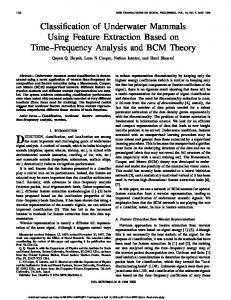
Figure 9: Time domain diagram of underwater noise.

Oim

xin n input neurons

M output neurons

After the value of 𝛽 is calculated, the training work of extreme learning machine classifier is finished. If a test sample 𝑋 of an unknown label is given, classification can be made by a well trained extreme learning machine classifier, whose category can be obtained by the calculation of formula (7):

M hidden layer neurons

Figure 8: Extreme learning machine classifier.

network, 𝑇𝑖 is the category label vector of number 𝑖 sample, 𝑤𝑖𝑗 is the weight vector connecting number 𝑖 sample and number 𝑗 neuron in hidden layer, 𝑏𝑗 is the bias of number 𝑗 neuron in hidden layer, and 𝑓(⋅) is activated function. Formula (4) can be written as the matrix form as shown in formula (5), and 𝐻𝑤,𝑥,𝑏 is called output matrix of hidden layer. 𝛽1𝑇

𝐻𝑤,𝑥,𝑏 𝛽 = 𝑇,

[ 𝑇] [ 𝑇] [𝛽 ] [𝑇 ] [ 2] [ 2] [ ] [ ] [ .. ] [ ] 𝛽 = [ . ] , 𝑇 = [ ... ] [ ] [ ] [ 𝑇] [ 𝑇] [𝛽 ] [𝑇 ] [ 1] [ 1] 𝑇 [𝛽𝑀]

𝐻𝑤,𝑥,𝑏

𝑇1𝑇

,

(5)

𝑇

[𝑇𝑁]𝑁×𝑀

𝑓 (𝑊1 ⋅ 𝑋1 + 𝑏1 ) ⋅ ⋅ ⋅ 𝑓 (𝑊𝑀 ⋅ 𝑋1 + 𝑏𝑀) [ ] [ ] .. .. =[ ] . (6) . d . [ ] 𝑓 (𝑊 ⋅ 𝑋 + 𝑏 ) ⋅ ⋅ ⋅ 𝑓 (𝑊 ⋅ 𝑋 + 𝑏 ) 1 𝑁 1 𝑀 𝑁 𝑀 ] [

What formula (5) expresses is a linear system. In case that the number of hidden layer neurons in the network is the same with the number of training sample, its output layer matrix is a square matrix, and it can be known from the two bold theories of Huang Guangbin that such square matrix is reversible; then the least square solution of such system is 𝛽 = 𝐻−1 𝑇. However, in fact, the number of nodes in hidden layer usually is less than the number of samples, so the matrix of output layer is not a square matrix. The least square solution of such linear system is 𝛽 = 𝐻+ 𝑇, in which, 𝐻+ is the generalized inverse matrix of 𝐻𝑤,𝑥,𝑏 . From the above analysis, we can see that the training process of the extreme learning machine classifier can be divided into the following three steps: (1) Initialize the input weight 𝑊𝑖 and bias 𝑏𝑖 (𝑖 = 1, 2, . . . , 𝑀) of the network at random; (2) Calculate the output matrix 𝐻𝑤,𝑥,𝑏 of the hidden layer and its generalized inverse matrix 𝐻+ ; (3) Calculate output weight 𝛽 by formula 𝛽 = 𝐻+ 𝑇.

𝑇𝑀 (𝑋) = 𝐻 (𝑋) 𝛽,

(7)

in which, 𝐻(𝑋) = [𝑓(𝑊1 , 𝑏1 , 𝑋) ⋅ ⋅ ⋅ 𝑓(𝑊𝑀, 𝑏𝑀, 𝑋)] is response of hidden layer to 𝑋.

5. Experiment Results and Analysis 5.1. Experiment Conditions and Parameters Setting. All experiments mentioned in this article are completed on the server of the laboratory, and the configuration of the server is as follows: 64 bits win 7 operation system, 64 GB memory, 24 cores of CPU and K40 GPU of NVIDIA Company, is equipped for accelerated calculation. Software used in the experiments is the latest version of MATLAB 2015a, latest version of VS2013, and the version of CUDA is 6.5. All data of the experiment come from the actual civil ship data samples. The experimental data come from the civil ship data sample, which is the waveform data from the original ship target radiated underwater noise passed through the sonar into the ADC converter output. Figure 9 shows a time domain diagram of the underwater acoustic signal of a civil boat sample and Figure 10 shows the frequency domain of the underwater acoustic signal of a civil boat sample. The colour scale represents energy and is measured in microvolts. Such dataset includes three kinds of civil ships, that is, small ship, big ship, and Bohai ferry, and the sampling place is the anchorage ground, and sampling frequency is 12800 Hz. In the experiment, eighty percent of each kind of samples are used as training set, and the rest twenty percent are used as test set. The feature extraction process of CNN involves large quantity of parameters, and this article gets the optimal network structure as shown in Table 1 through numerous experiments. In order to facilitate the programming realization, the full connection process is equivalent to using a convolutional kernel of 1∗1 to sum the convolution of all upper feature figures, and the number of feature figures equals to the number of neurons in current layer of full connection network. The first pool layer chooses maximum value pooling, and the second pool layer chooses mean value pooling. The combination of maximum value pooling and mean value pooling will


7 Table 1: CNN structure parameters.

Type Input layer Convolutional layer Sampling layer Convolutional layer Sampling layer Convolutional layer Full connection Full connection Full connection

Frequency (Hz)

Layer number (1) (2) (3) (4) (5) (6) (7) (8) (9)

Number of feature figures 1 64 64 128 128 500 2000 100 3

Size of feature figures 2176 ∗ 1 79 ∗ 1 39 ∗ 1 28 ∗ 1 14 ∗ 1 1∗1 1∗1 1∗1 1∗1

6000

Length of step — 25 2 1 2 1 1 1 1

0

4000

−50

2000 0

Size of kernel — 204 ∗ 1 2∗1 12 ∗ 1 2∗1 14 ∗ 1 1∗1 1∗1 1∗1

−100 0

50

100

150

200 250 Time (s)

300

350

400

Figure 10: Frequency domain diagram of underwater noise.

Table 2: Value choice and selection of typical parameters. Parameters Activated functions Size of learning rate Decay rate of learning rate Number of batch processing samples (Batch) Impulse magnitude

Scope ReLu 0.02∼0.05 0.0005/Batch 200 0.9

achieve better effects. The typical parameter value choice and selection involved in neural network training process are shown in Table 2. 5.2. Experiment Analysis. In pooling process, there are two commonly seen pooling methods: mean value pooling and maximum value pooling. This article compares the two different pooling methods and the chosen classifiers are all the extreme learning machines. The experiment results are shown in Table 3. Table 3 shows that choosing different pooling method in the pooling process has a big impact on the features extracted. The performance with both pool layers using mean value pooling is the worst one, while the combination of mean value pooling and maximum value pooling in the pooling process can achieve an ideal effect; besides, the effect with the last pool layer of the network using mean value pooling is superior to the one using maximum value pooling. This article compares the traditional “manual features” (Mel frequency cepstrum coefficient feature and HilbertHuang transform feature) and the features “automatically” extracted by deep convolutional networks as used by this article. All the classifiers chosen in the experiment are extreme learning machine classifiers; however, number of

neurons in hidden layer of extreme learning machine and the activated functions used by the learning machine are different. The experiment results are shown in Table 4. The Table 4 experiment shows that the features obtained by extracting the features of original sound signals through deep learning are effective, and the ELM algorithm can be used to realize separation to civil ship sound signals, and the recognition rate on the test set can reach 93.04%. Compared with traditional MFCC features and the features obtained from Hilbert-Huang transform, the features obtained from deep learning are easier to be classified. As to the recognition rate, the rates obtained from features adopted by this article are 5%∼10% higher than those obtained from traditional features, which is mainly because the traditional features are the ones generated “manually,” without fully considering the inner links of signal, while deep learning can realize “automatic” extraction of features. Besides, comparison is made on different features of extreme learning machine classifier mentioned in the article and traditional classifier. In such experiment, number of hidden layer neurons of extreme learning machine is 40, and Tables 5 and 6, respectively, give the effects of the three different classifiers on classification and recognition of MFCC features and features obtained from deep learning. In Table 6, both the training time and test time refer to mean time of single samples. It can be seen intuitionally from the table that though K neighboring classifier and SVM classifier can realize feature space division, the recognition rates of the two obviously are lower than the recognition rate of ELM classifier; what is more, training time and test time of the two far exceed the time used by ELM. The analysis made in the comparison experiment in Table 4 shows that the features obtained from “automatic” feature extraction using deep convolutional networks are

8

Computational Intelligence and Neuroscience Table 3: Comparison of different pooling methods.

Frame size 2176 2176 2176 2176

Pooling method Maximum value Mean value Maximum value-mean value Mean value-maximum value

Number of ELM hidden layer nodes 40 40 40 40

Recognition rate (%) 92.88 90.80 93.04 91.65

Table 4: Comparison of classification effects of different features. Feature types MFCC

HHT

Deep learning feature

Number of hidden layer neurons 40 60 80 60 40 60 40 60 40 60 20 40 60

ELM activated functions Sigmoid Sigmoid Sigmoid tanh Sigmoid Sigmoid tanh tanh Sigmoid Sigmoid tanh tanh tanh

Recognition rates (%) 84.64 84.48 84.41 82.39 81.06 82.34 81.72 82.04 90.39 92.69 92.40 93.04 92.29

Table 5: Comparison of performance of different classifiers (MFCC features). Names of classifier ELM SVM KNN

Training time (S) 3.73 × 10−5 1.69 × 10−4 —

Time of classification (S) 1.37 × 10−5 5.88 × 10−5 5.00 × 10−5

Recognition rate (%) 84.64 80.67 78.66

Table 6: Comparison of performance of different classifiers (convolutional networks features). Names of classifiers ELM SVM KNN

Training time (s) 3.82 × 10−5 1.12 × 10−4 —

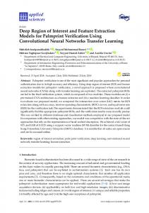
superior to the traditional features generated “manually”; however, a model extracted by using neural network is an issue worthy of thinking. Making an analysis on all parameters in the network obviously is not possible; however, we can analyze and process the convolutional kernels learnt from convolutional layer. Figure 11 gives part of the convolutional kernels obtained through learning in the first convolutional layer in the convolutional neural networks. The X-axis means the sequence number of the convolution kernel sequence, while the Y-axis means the value of the convolution kernel sequence. Apparently, these convolutional kernels serve as one and another band-pass filters and, respectively, respond to different frequency bands of transmission signals, and the convolutional kernels obtained from these learnings can be regarded as a matched filter. Through making research on the amplitude frequency features of the convolutional kernels

Time of classification (s) 1.24 × 10−5 4.05 × 10−5 9.73 × 10−5

Recognition rates (%) 93.04 82.67 86.67

obtained, we find that these filters are distributed nonlinearly and mostly located in low frequency band. It can be seen from Figure 11 that the useful components of the underwater noise signal of a civil ship are concentrated in the low frequency part of the frequency domain.

6. Conclusion This article conducts feature extraction to original waveform of underwater sound signal by adopting deep convolutional neural networks and takes the extracted features as the input features of extreme learning machine classifier and realizes the classification and recognition to underwater sound signals. This article compares the feature extraction method set forth in this article and the traditional feature extraction methods and validates the effectiveness of the


9

Filter 17

0.6

Filter 42

−0.02

0.4

Weight

Weight

−0.04 0.2

−0.06 0

−0.2

0

100

200

−0.08

300

0

100

Filter 44

0.2

200

300

0.2

Weight

Weight

300

Filter 56

0.4

0.1

0

0

−0.2

−0.1

−0.2

200 Simple

Simple

0

100

200

300

−0.4

0

100 Simple

Simple

Figure 11: The coefficients of some convolution kernels.

feature extraction methods used herein. Meanwhile, this article compares the classification effects and classification times of different classifiers at the classifier stage and highlights the advantages of the classifier used by this article in classification time and classification precision. Compared with the traditional MFCC and HTT, the recognition rate of 93.04% has been greatly improved on the actual civil ship data set. Experimental results show that CNN can be better used to extract the feature extraction and recognition of underwater target noise data.

Conflicts of Interest The authors declare that they have no conflicts of interest.

Acknowledgments This work is supported by the Underwater Measurement and Control Foundation of Key Laboratory (no. 9140C260505150C26115).

References [1] Y. LeCun, Y. Bengio, and G. Hinton, “Deep learning,” Nature, vol. 521, no. 7553, pp. 436–444, 2015. [2] A.-R. Mohamed, G. E. Dahl, and G. Hinton, “Acoustic modeling using deep belief networks,” IEEE Transactions on Audio, Speech and Language Processing, vol. 20, no. 1, pp. 14–22, 2012. [3] J. Chen, Y. Wang, and D. Wang, “A feature study for classification-based speech separation at low signal-to-noise ratios,” IEEE/ACM Transactions on Audio Speech and Language Processing, vol. 22, no. 12, pp. 1993–2002, 2014. [4] Y. Jiang, D. L. Wang, R. S. Liu, and Z. M. Feng, “Binaural classification for reverberant speech segregation using deep neural networks,” IEEE/ACM Transactions on Audio Speech and Language Processing, vol. 22, no. 12, pp. 2112–2121, 2014. [5] C. Cortes and V. Vapnik, “Support-vector networks,” Machine Learning, vol. 20, no. 3, pp. 273–297, 1995. [6] L. E. Peterson, “K-nearest neighbor,” Scholarpedia, vol. 4, no. 2, article 1883, 2009. [7] N. E. Huang and S. P. Shen, Hilbert-Huang Transform and Its Applications, World Scientific, Singapore, 2005.

10 [8] A. Jain and H. Harris, Speaker Identification Using MFCC and HMM Based Techniques, University of Florida, 2004. [9] Q.-J. Zeng, F. Wang, and G.-J. Huang, “Technique of passive sonar target recognition based on continuous spectrum feature extraction,” Journal of Shanghai Jiaotong University, vol. 36, no. 3, pp. 382–386, 2002. [10] S. Zhi-guang, H. Chuan-jun, and C. Sheng-yu, “Feature extraction of ship radiated noise base on wavelet multi-resolution decomposition,” Qingdao University, vol. 16, no. 4, pp. 44–48, 2003. [11] Z. Hua-xin and Z. Ming-xiao, “Researches on chaotic phenomena of noises radiated from ships,” ACTA ACUSTICA, vol. 23, no. 2, pp. 134–140, 1998. [12] X.-K. Li, L. Xie, and Y. Qin, “Underwater target feature extraction using Hilbert-Huang transform,” Journal of Harbin Engineering University, vol. 30, no. 5, pp. 542–546, 2009. [13] G. E. Hinton and R. R. Salakhutdinov, “Reducing the dimensionality of data with neural networks,” American Association for the Advancement of Science: Science, vol. 313, no. 5786, pp. 504–507, 2006. [14] H. Lee, L. Yan, P. Pham, and A. Y. Ng, “Unsupervised feature learning for audio classification using convolutional deep belief networks,” in Proceedings of the 23rd Annual Conference on Neural Information Processing Systems (NIPS ’09), vol. 9, pp. 1096–1104, December 2009. [15] N. Jaitly and G. Hinton, “Learning a better representation of speech soundwaves using restricted boltzmann machines,” in Proceedings of the 36th IEEE International Conference on Acoustics, Speech, and Signal Processing, (ICASSP ’11), pp. 5884– 5887, May 2011. [16] G. Hinton, L. Deng, D. Yu et al., “Deep neural networks for acoustic modeling in speech recognition: the shared views of four research groups,” IEEE Signal Processing Magazine, vol. 29, no. 6, pp. 82–97, 2012. [17] D. Palaz, R. Collobert, and M. Magimai-Doss, “Estimating phoneme class conditional probabilities from raw speech signal using convolutional neural networks,” in Proceedings of the 14th Annual Conference of the International Speech Communication Association, INTERSPEECH 2013, pp. 1766–1770, August 2013. [18] Y. LeCun, B. Boser, J. S. Denker et al., “Backpropagation applied to handwritten zip code recognition,” Neural Computation, vol. 1, no. 4, pp. 541–551, 1989. [19] O. Abdel-Hamid, A.-R. Mohamed, H. Jiang, L. Deng, G. Penn, and D. Yu, “Convolutional neural networks for speech recognition,” IEEE Transactions on Audio, Speech and Language Processing, vol. 22, no. 10, pp. 1533–1545, 2014. [20] G. B. Huang, Q. Y. Zhu, and C. K. Siew, “Extreme learning machine: a new learning scheme of feedforward neural networks,” in Proceedings of the IEEE International Joint Conference on Neural Networks, vol. 2, pp. 985–990, July 2004. [21] G. Huang, G.-B. Huang, S. Song, and K. You, “Trends in extreme learning machines: A review,” Neural Networks, vol. 61, pp. 32– 48, 2015.


Journal of

Advances in

Industrial Engineering

Multimedia

Hindawi Publishing Corporation http://www.hindawi.com

The Scientific World Journal Volume 2014


Volume 2014

Applied Computational Intelligence and Soft Computing

International Journal of

Distributed Sensor Networks Hindawi Publishing Corporation http://www.hindawi.com

Volume 2014


Volume 2014


Volume 2014

Advances in

Fuzzy Systems Modelling & Simulation in Engineering Hindawi Publishing Corporation http://www.hindawi.com


Volume 2014

Volume 2014

Submit your manuscripts at https://www.hindawi.com

Journal of

Computer Networks and Communications

Advances in

Artificial Intelligence Hindawi Publishing Corporation http://www.hindawi.com


Volume 2014


Biomedical Imaging

Volume 2014

Advances in

Artificial Neural Systems


Computer Engineering

Computer Games Technology



Advances in

Volume 2014

Advances in

Software Engineering Volume 2014


Volume 2014


Volume 2014


Volume 2014


Reconfigurable Computing

Robotics Hindawi Publishing Corporation http://www.hindawi.com


Advances in

Human-Computer Interaction

Journal of

Volume 2014


Volume 2014


Journal of

Electrical and Computer Engineering Volume 2014


Volume 2014


Volume 2014