Deep Learning with Cinematic Rendering - Fine ...

Deep Learning with Cinematic Rendering Fine-Tuning Deep Neural Networks Using Photorealistic Medical Images Faisal Mahmooda , Richard Chenb , Sandra Sudarskyc , Daphne Yuc , Nicholas J. Durra a Department

of Biomedical Engineering, Johns Hopkins University, Baltimore, MD of Computer Science, Johns Hopkins University, Baltimore, MD c Siemens Healthineers, Medical Imaging Technologies, Princeton, NJ, USA

b Department

Abstract Deep learning has emerged as a powerful artificial intelligence tool to interpret medical images for a growing variety of applications. However, the paucity of medical imaging data with high-quality annotations that is necessary for training such methods ultimately limits their performance. Medical data is challenging to acquire due to privacy issues, shortage of experts available for annotation, limited representation of rare conditions and cost. This problem has previously been addressed by using synthetically generated data. However, networks trained on synthetic data often fail to generalize to real data. Cinematic rendering simulates the propagation and interaction of light passing through tissue models reconstructed from CT data, enabling the generation of photorealistic images. In this paper, we present one of the first applications of cinematic rendering in deep learning, in which we propose to fine-tune synthetic data-driven networks using cinematically rendered CT data for the task of monocular depth estimation in endoscopy. Our experiments demonstrate that: (a) Convolutional Neural Networks (CNNs) trained on synthetic data and finetuned on photorealistic cinematically rendered data adapt better to real medical images and demonstrate more robust performance when compared to networks with no fine-tuning, (b) these fine-tuned networks require less training data to converge to an optimal solution, and (c) fine-tuning with data from a variety of photorealistic rendering conditions of the same scene prevents the network from learning patient-specific information and aids in generalizability of the model. Our empirical evaluation demonstrates that networks fine-tuned with cinematically rendered data predict depth with 56.87% less error for rendered endoscopy images and 27.49% less error for real porcine colon endoscopy images. Keywords: Convolutional Neural Networks, Deep Learning, Synthetic Data, Synthetic Medical Images, Cinematic Rendering, Transfer Learning, Fine Tuning, Endoscopy, Endoscopy Depth Estimation

Preprint submitted to Physics in Medicine and Biology.

May 22, 2018

1. Introduction Convolutional Neural Networks (CNNs) have revolutionized the fields of computer vision, machine and automation, achieving remarkable performance on previously-difficult tasks such as image classification, semantic segmentation, and depth estimation. [45, 16, 44, 55]. CNNs are particularly powerful in supervised learning tasks where it is difficult to build an accurate mathematical model for the task at hand. With recent improvements made in training CNNs such as utilizing dropout regularization, skip connections and the advancements made in high-performance computing due to graphical processing units [24, 14], deep learning models have become much easier to train and vastly more accessible. To achieve generalization, deep learning models require large amounts of data that are accurately annotated. Obtaining such a dataset for a variety of medical images is challenging because expert annotation can be expensive, time consuming [18, 29], and often limited by the subjective interpretation [23]. Moreover, other issues such as privacy and under-representation of rare conditions impede developing such datasets [53, 43]. This is supplemented with the cross-patient adaptability problem, where networks trained on data from one patient fail to adapt to another patient [38, 26]. For medical diagnostics, physicians are interested in diagnostic information which is common across patients rather than patient-specific information. 1.1. Training with Synthetic Medical Images Recently, the limited availability of medical data has been addressed by the use of synthetic data [27, 26, 28]. Computer graphics engines such as Blender and Unreal have the ability to construct realistic virtual worlds, but are limited by the diversity of 3D assets to create accurate, tissue-equivalent models [56]. Other methods for synthetic data generation include Generative Adversarial Networks (GANs), which train a generative deep network to learn and sample a target distribution of realistic images [15]. This approach, however, suffers from the mode collapse problem, a commonly encountered failure case in GANs where the support size of the learned distribution is low, and thus, the generated images are sampled with low variability [7]. Overall, networks trained on synthetic data often fail to generalize to real data, as both of these approaches in synthetic data generation fail to produce realistic, diverse examples necessary for training deep networks in medical images [26]. Cinematic rendering is a recently developed visualization technique that works by simulating the propagation and interaction of light passing through tissue models reconstructed from cross-sectional images such as CT, enabling the generation of photorealistic images that have not previously been possible [11]. In this paper, we use cinematic rendering to generate a wide range of healthy to pathologic colon tissue with ground truth depth, and fine-tune synthetic data-driven networks with these images to address the problem of the cross-patient adaptability in training deep networks. To our knowledge, this is the first application of cinematic rendering in deep learning for medical image analysis. We test this method for monocular

2

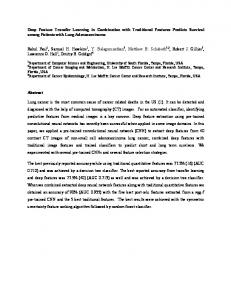
Figure 1: Data generation process for (a) Synthetically generated data for training (b) Cinematically rendered data for fine-tuning and (c) Pig colon data for validation.

depth estimation in endoscopy, a task with many clinical applications [10] but is challenging to acquire accurately. 1.2. Fine-Tuning Deep Networks CNNs are trained by solving a typically non-convex error function using local search algorithms such as stochastic gradient descent and other optimizations. Beginning with randomly initialized weights, CNNs seek to minimize their empirical risk over the training dataset by iteratively updating the network parameters in the opposite direction of its error gradient, such that the network’s performance converges towards a minimum on the loss surface [2]. With limited data, poor initialization, and a lack of regularization to control capacity, the network may fail to generalize, and convergence can become slow when traversing saddle points and also lead to sub-optimal local minima [32, 3, 54, 8, 42]. Initializing weights from a CNN trained for a similar task with a much larger dataset however, allows the network to converge much more easily to a good local minima and necessitates less labeled data [13]. This process is called transfer learning, and is widely used in classification and segmentation tasks such as lesion detection in medical imaging, where there exists a paucity of annotated data [35, 1, 12, 46, 57, 41]. In practice, transfer learning involves

3

Figure 2: Representative images of synthetically generated endoscopy data with ground truth depth for training (top), cinematically rendered CT data with ground truth depth for finetuning (middle) and real endoscopy data with ground truth depth from registered CT views for testing (bottom).

transferring weights from an existing network trained on a much larger dataset. For networks trained on similar tasks and datasets, the new network would freeze the first few layers, and train the remaining layers at a low learning rate. This process is called fine-tuning. Intuitively, the first few layers of a CNN hold low-level features that are shared across all types of images, and the last layers hold high-level features that are learned for a specific application [49, 58, 41]. In this specific context, we hypothesize that networks trained on synthetic medical data, that might not have previously adapted to real data, would generalize better if fine-tuned using cinematically rendered photorealistic data. We further hypothesize that such fine-tuned networks require less amount of training data, and would work well in low-resource settings such as endoscopy. 1.3. Depth Estimation for Endoscopy For the purpose of validating our hypotheses we focus on the task of depth estimation from monocular endoscopy images. Monocular depth estimation from endoscopy is a challenging problem and has a variety of clinical applications including topographical reconstruction of the lumen, image-guided surgery, endoscopy quality metrics, and enhanced polyp detection, as polyps can lie on convex surfaces and can be occluded by folds in the gastrointestinal tract [19, 59, 52]. Depth estimation is especially challenging because the tissue being imaged is often deformable, and endoscopes have a single camera with close light sources and a wide field of view. Current approaches either have limited accuracy due to 4

restrictive assumptions [20] or require modifying endoscope hardware which has significant regulatory and engineering barriers [34, 9]. Data-driven approaches for depth estimation in endoscopy are additionally complicated because of the lack of clinical images with available ground truth data, since it is difficult to include a depth sensor on an endoscope [30]. Moreover, networks trained on data from one patient fail to generalize to other patients since they start learning from patient-specific texture and color. Previous work has focused on generating synthetic data and adversarial domain adaptation to overcome these issues [27, 26]. In this paper, we will focus on using synthetic endoscopy data with ground truth depth for training and fine-tuning using photorealistic cinematically rendered data. 2. Methods 2.1. Endoscopy Depth Dataset Generation We generated three different datasets of endoscopy images with ground truth depth for three different purposes: (a) a large dataset of synthetic endoscopy images for training, (b) a small dataset of cinematically rendered images for fine-tuning, and (c) a small dataset of real endoscopy images of a porcine colon for validation. 2.1.1. Synthetic Endoscopy Data for Training Though synthetic data has been extensively used to train deep CNN models for real-world images [48, 17, 51, 36], this approach has been relatively limited for medical imaging. Recent work in generating synthetic data for medical images have been applying GANs to retinal images and histopathology images [6]. However, GANsynthesized medical data does not cater for the cross-patient adaptability problem. In general, synthetic medical imaging data can be generated given an anatomically correct organ model and a forward model of an imaging device (Fig. 1-Top). Forward models for diagnostic imaging devices are more complicated than typical cameras and anatomic models of organs need to represent a high degree of variation. We developed a forward model of an endoscope with a wide-angle monocular camera and two to three light sources that exhibit realistic inverse square law of intensity fall-off. We use a synthetically-generated and anatomically accurate colon model and image it using the virtual endoscope placed at a variety of angles and varying conditions to mimic the movement of an actual endoscope. We also generate pixel-wise ground truth depth for each rendered image. Using this model, we generated a dataset of 200,000 grayscale endoscopy images, each with a corresponding, perfect-accuracy ground truth depth map (Fig. 1-Top, Fig. 2).

5

2.2. Cinematically Rendered Data for Fine-Tuning The Cinematic VRT technology developed at Siemens Healthcare provides a natural and photorealistic 3D representation of medical scans, such as Computed Tomography (CT) or Magnetic Resonance Images (MRI) [5]. The physical rendering algorithm, based on a Monte Carlo path-tracing technique closely simulates the complex interaction of light rays with tissues found in the scanned volume. Compared to traditional volume ray casting, where only light emission and absorption along a straight ray is considered, path tracing considers light paths with multiple random scattering events and light extinction. Although this lighting model requires more computational power as hundreds of light paths must be calculated, it considerably enhances depth and shape perception. By putting the anatomical structures within the medical scans in a virtual lighting condition that mimics the physical lighting experienced in reality, soft shadows, ambient occlusions and volumetric scattering effects can be observed in the cinematic rendered images. Monte Carlo path tracing and interaction can be used to calculate the radiant flux, L at a distance x received from the direction ω along a ray using the following multidimensional rendering equation, Z  Z D −τ (x,x0 ) 0 0 0 0 0 (1) L(x, ω) = e σs (x ) p(ω, ω )Li (x , ω )dω dx0 , 0

Ω4π

0

where, ω represents all possible light directions and D represents the maximum distance. The optical properties of the tissue under consideration are defined by p(ω, ω 0 ), which describes the fraction of light traveling along a direction ω 0 being scattered into direction ω.Li (x0 , ω 0 ) is the radiance arriving at distance x0 from direction ω 0 . Surface interactions are modeled with a bidirectional reflectance distribution function (BRDF) and tissue scattering is modeled using R x0 a Henyey-Greenstein phase function [50]. τ (x, x0 ) = x σt (t)dt represents the optical depth and its corresponding excitation coefficient is represented by the sum of absorption and scattering coefficients, σt = σs + σa [5]. Compared to conventional medical rendering, this technique considerably enhances depth and shape perception by putting the anatomical structures within the medical scans in a virtual lighting condition that mimics the physical lighting experienced in reality. Cinematic rendering has been used for a variety of medical imaging visualization tasks [22, 40, 4, 39]. Using this Cinematic VRT technology, colonic images were generated together with their corresponding depth maps, by saving the gradient and the position of the rays once their accumulated opacity had reached a given threshold (Fig. 1-Middle). Four different sets of rendering parameters were used to generate a diverse set of renderings for each scene. This was done to prevent the network from learning texture and color in the renderings (Fig. 1-Middle, Fig. 2). We used a total of 1200 rendered images for fine-tuning from 300 different scenes. The CT colonoscopy data used was acquired from the NIH Cancer Imaging Archive (TCIA) [21].

6

Figure 3: Architecture of a CNN-CRF network with fine-tuning. The unary part is composed of 5 convolutional and 4 fully connected layers and the pairwise part is composed of a fully convolutional layer. Repeating units of this setup can be used for parallel processing.

2.3. Real Pig Colon Optical Endoscopy Data To validate our approach, we tested the depth-estimation performance on a dataset of real endoscopy images. We created a dataset of ex-vivo pig colon optical endoscopy images with ground truth depth determined from CT. In particular, we fixed a porcine colon to a tubular scaffold and conducted optical endoscopy imaging using a Misumi Endoscope (MO-V5006L). Subsequently, we collected cone beam CT data from the same scaffold. A 3D model of this fixed colon was reconstructed using filtered-back projection with a Ram-Lak filter [31]. The reconstructed density was then imaged using a virtual endoscope with same camera parameters as the optical Misumi endoscope. The resulting virtual endoscopy images were registered to optical endoscopy views using a one-plusone evolutionary optimizer [47, 60]. Once registered, the depth for each virtual endoscopy view was used as the depth for the corresponding optical endoscopy view (Fig.1-Bottom, Fig. 2). 2.4. Monocular Endoscopy Depth Estimation using CNN-CRF Joint Training To train an endoscopy depth estimation network using synthetic data and fine-tuning using cinematically rendered data we used a joint CNN and Conditional Random Fields (CRF) network similar to the setup described in [27, 25]. Intuitively, a CNN-CRF setup is more context-aware than a simple CNN, as it takes into account the smooth transitions and abrupt changes that are characteristic of an endoscopy depth map. Assuming g ∈ Rn×m is an endoscopy image which has been split into super-pixels, p, and y = [y1 , y2 , ..., yp ] ∈ R is the depth for each super-pixel. The conditional probability can be stated as, exp(E(y, x)) . exp(E(y, x))dy −∞

P r(y|x) = R ∞

7

(2)

where, E is the energy function of the conditional random fields. In order to predict the depth of a new image we need to solve a maximum aposteriori b = argmaxy P r(y|x). problem, y Let ξ and η be unary and pairwise potentials respectively represented over nodes N and edges S of x, the overall energy function can be simplified as, X X E(y, x) = ξ(yi , x; θ) + η(yi , yj , x; β), (3) i∈N

(i,j)∈S

where, ξ predicts the depth from a super-pixel and η encourages smoothness between pairwise superpixels. The two potentials are learned in a unified framework. As suggested in [25] the unary function is, ξ(yi , x; θ) = −(yi − hi (θ))2

(4)

where hi is the predicted depth of a superpixel and θ represents CNN parameters. The pairwise potential function is based on standard CRF models. Assuming β to be the parameters of the network and S be the similarity index k matrix where Si,j represents a similarity association metric between the ith and th j super-pixel. In this specific case, intensity and greyscale histogram was used to represent pairwise similarities. The pairwise potential can be written as, K 1X k (5) βk Si,j (yi − yj )2 . η(yi , yj ; β) = − 2 k=1

Simplifying the energy function, K X 1 X X k βk Si,j (yi − yj )2 . E=− (yi − hi (θ))2 − 2 i∈N

(6)

(i,j)∈S k=1

During the joint CNN-CRF training process the negative log likelihood of the probability density function which can be simplified from Eq. 1 is minimized with respect to the two learning parameters. Weight decay parameters (λθ , λβ ) were added to the objective function to reduce the influence of heavily weighted vectors. Let N be the number of images in the training data then the objective function can be written as, N X λθ λβ 2 2 (7) min − log P r(y|x; θ, β) + kθk2 + kβk2 . θ,β≥0 2 2 1 This joint CNN-CRF optimization problem is solved using stochastic gradient decent-based back propagation. Our network operates for the unary part on a 224 × 224 superpixel patch level and is composed of 5 convolutional and 4 fully connected layers (Fig. 3). The fully connected layers are fine-tuned using cinematically rendered data. The network architecture is illustrated in Fig. 3.

8

3. Results 3.1. Quantitative Evaluation We evaluated based on metrics our depth estimation paradigm and the capability of fine-tuning using the following metrics: P |y −y | 1. Relative Error (rel): N1 y gtygt est P 2. Average log10 Error (log10 ): N1 y |log10 ygt − log10 yest | q P 3. Root Mean Square Error (rms): N1 y (ygt − yest )2 Where ygt is the ground truth depth yest is the estimated depth and N is the total number of samples. Table 1 and 2 and Fig. 4 show results based on these metrics for cinematically data and porcine colon real endoscopy data. None of the test data was or images within the close proximity were used for training. Tables I and II validate our hypotheses that CNN-CRF fine-tuned networks (CNN-CRF-FT) works better than networks trained only on synthetic data and that a smaller amount of data is required for initial full training if the last layers are fine-tuned. We also observed that fine-tuning with four renderings of a scene improved performance over fine-tuning with just one rendering (Table 2). This is likely because in supplying multiple renderings of the same scene with the same depth map, the CNN-CRF was able to better learn the context-aware features for depth estimation such as intensity differences between superpixels, and overcome noisy details such as texture or color. As a result, the network was able to work well on real data such as the pig colon data used in this study. Table 3 shows that fine-tuning with just 300 images from one kind of rendering gives a worse result compared to fine-tuning with 75 images each from four different kinds of renderings. Table 1: Performance Evaluation for Cinematically Rendered Endoscopy Images

Method

Training

Fine-Tuning

rel ↓

log10 ↓

rms ↓

CNN-CRF CNN-CRF-FT CNN-CRF CNN-CRF-FT

200,000 200,000 100,000 100,000

None 1200 None 1200

0.394 0.166 0.477 0.189

0.241 0.078 0.319 0.081

1.933 0.708 2.590 0.756

4. Conclusion Despite the recent advances in computer vision and deep learning algorithms, their applicability to medical images is often limited by the scarcity of annotated data. The problem is further complicated by the underrepresentation of rare conditions. For example, getting annotated data for polyp localization is difficult because in a 20 minute colonoscopy examination of the 1.5 meter colon, only 9

Figure 4: Representative images of estimated depth and corresponding ground truth depth for cinematically rendered data and real pig colon endoscopy data.

10

Table 2: Performance Evaluation for Real Pig Colon Endoscopy Images

Method

Training

Fine-Tuning

rel ↓

log10 ↓

rms ↓

CNN-CRF CNN-CRF-FT CNN-CRF CNN-CRF-FT

200,000 200,000 100,000 100,000

None 1200 None 1200

0.411 0.298 0.495 0.329

0.258 0.171 0.392 0.196

2.318 1.387 2.897 1.714

Table 3: Performance Evaluation for Fine-Tuning with One vs Four Different Rendering (Pig Colon Data)

Method

Training

Fine-Tuning

rel ↓

log10 ↓

rms ↓

CNN-CRF-FT (1 × 300) CNN-CRF-FT (4 × 75)

200,000 200,000

300 300

0.471 0.364

0.363 0.221

2.614 2.153

a few 10 mm polyps may be present. Depending on the field-of-view of the camera, the polyps may also be occluded by folds in the gastrointestinal tract [52]. Using depth with RGB images has shown to improve localization in natural scenes by helping recover rich structural information with less annotated data and better cross-dataset adaptability [19]. Within the constrained setting of endoscopy, estimating depth from monocular views is difficult because ground truth depth is hard to acquire. Problems where ground truth is difficult or impossible to acquire have been tackled for natural scenes by generating synthetic data. However, there are few examples of synthetic data driven medical imaging applications [26, 27, 33]. This is because synthetic data-driven models often fail to generalize to the real datasets, and is often complimented by the cross patient network adaptability problem, where networks that work well on one patient do not generalize to other patients. In this work, we demonstrate one of the first successful uses of cinematically rendered data for generalizing a network trained on synthetic data to real data. Additionally, our approach successfully addresses the issue of the cross-patient adaptability. We show that a synthetic data-driven CNN-CRF model can be successfully trained for accurate depth estimation on real tissue given no real optical endoscopy training data. Beyond accurate depth estimation, future work will investigate semantic segmentation in endoscopy by fusing depth as an additional input [19]. Our future work will also focus on generalizing this concept to other medical imaging modalities. Acknowledgments The authors would like to thank Sermet Onel for his help with internal lighting and Kaloian Petkov for his help with multiple aspects of the cinematic renderer.

11

Disclaimer This feature is based on research, and is not commercially available. Due to regulatory reasons its future availability cannot be guaranteed. References [1] Azizpour H, Razavian A S, Sullivan J, Maki A and Carlsson S 2015 in ‘CVPRW DeepVision Workshop, June 11, 2015, Boston, MA, USA’ IEEE conference proceedings. [2] Bottou L 2010 in ‘Proceedings of COMPSTAT’2010’ Springer pp. 177–186. [3] Choromanska A, Henaff M, Mathieu M, Arous G B and LeCun Y 2015 in ‘Artificial Intelligence and Statistics’ pp. 192–204. [4] Chu L C, Johnson P T and Fishman E K 2018 Abdominal Radiology pp. 1–7. [5] Comaniciu D, Engel K, Georgescu B and Mansi T 2016 Medical image analysis 33, 19– 26. [6] Costa P, Galdran A, Meyer M I, Niemeijer M, Abr` amoff M, Mendon¸ca A M and Campilho A 2017 IEEE Transactions on Medical Imaging . [7] Creswell A, White T, Dumoulin V, Arulkumaran K, Sengupta B and Bharath A A 2018 in ‘IEEE Signal Processing Magazine’ Vol. 35 pp. 53–65. [8] Dauphin Y N, Pascanu R, Gulcehre C, Cho K, Ganguli S and Bengio Y 2014 in ‘Advances in neural information processing systems’ pp. 2933–2941. [9] Durr N J, Gonzlez G, Lim D and Traverso G 2014 in ‘Advanced Biomedical and Clinical Diagnostic Systems’ Vol. 8935 International Society for Optics and Photonics. [10] Durr N J, Gonzlez G and Parot V 2014 Expert Review of Medical Devices 11(2), 105– 107. [11] Eid M, Cecco C N D, Nance J W, Jr., Caruso D, Albrecht M H, Spandorfer A J, Santis D D, Varga-Szemes A and Schoepf U J 2017 American Journal of Roentgenology 209(2). [12] Girshick R, Donahue J, Darrell T and Malik J 2014 in ‘Proceedings of the IEEE conference on computer vision and pattern recognition’ pp. 580–587. [13] Glorot X and Bengio Y 2010 in ‘Proceedings of the thirteenth international conference on artificial intelligence and statistics’ pp. 249–256. [14] Goodfellow I, Bengio Y, Courville A and Bengio Y 2016 Deep learning Vol. 1 MIT press Cambridge. [15] Goodfellow I, Pouget-Abadie J, Mirza M, Xu B, Warde-Farley D, Ozair S, Courville A and Bengio Y 2014 in ‘Advances in neural information processing systems’ pp. 2672– 2680. [16] Greenspan H, van Ginneken B and Summers R M 2016 IEEE Transactions on Medical Imaging 35(5), 1153–1159. [17] Gupta A, Vedaldi A and Zisserman A 2016 in ‘Proceedings of the IEEE Conference on Computer Vision and Pattern Recognition’ pp. 2315–2324. [18] Gur Y, Moradi M, Bulu H, Guo Y, Compas C and Syeda-Mahmood T 2017 in ‘Intravascular Imaging and Computer Assisted Stenting, and Large-Scale Annotation of Biomedical Data and Expert Label Synthesis’ Springer pp. 87–95. [19] Hazirbas C, Ma L, Domokos C and Cremers D 2016 in ‘Asian Conference on Computer Vision’ Springer pp. 213–228. [20] Hong D, Tavanapong W, Wong J, Oh J and De Groen P C 2014 Computerized Medical Imaging and Graphics 38(1), 22–33. [21] Johnson C D, Chen M H, Toledano A Y, Heiken J P, Dachman A, Kuo M D, Menias C O, Siewert B, Cheema J I, Obregon R G et al. 2008 New England Journal of Medicine 359(12), 1207–1217. [22] Johnson P T, Schneider R, Lugo-Fagundo C, Johnson M B and Fishman E K 2017 American Journal of Roentgenology 209(2), 309–312. [23] Kerkhof M, Van Dekken H, Steyerberg E, Meijer G, Mulder A, De Brune A, Driessen A, Ten Kate F, Kusters J, Kuipers E and Siersema P 2007 Histopathology 50, 920–927. [24] LeCun Y, Bengio Y and Hinton G 2015 nature 521(7553), 436.

12

[25] Liu F, Shen C, Lin G and Reid I 2016 IEEE transactions on pattern analysis and machine intelligence 38(10), 2024–2039. [26] Mahmood F, Chen R and Durr N J 2017 arXiv preprint arXiv:1711.06606 . [27] Mahmood F and Durr N J 2017 arXiv preprint arXiv:1710.11216 . [28] Mahmood F and Durr N J 2018 in ‘Medical Imaging 2018: Image Processing’ Vol. 10574 International Society for Optics and Photonics p. 1057421. [29] Moradi M, Guo Y, Gur Y, Negahdar M and Syeda-Mahmood T 2016 in ‘International Conference on Medical Image Computing and Computer-Assisted Intervention’ Springer pp. 300–307. [30] Nadeem S and Kaufman A 2016 in ‘SPIE Medical Imaging’ International Society for Optics and Photonics pp. 978525–978525. [31] Natterer F 1986 The mathematics of computerized tomography Vol. 32 Siam. [32] Neyshabur B, Bhojanapalli S, McAllester D and Srebro N 2017 in ‘Advances in Neural Information Processing Systems’ pp. 5949–5958. [33] Nie D, Trullo R, Lian J, Petitjean C, Ruan S, Wang Q and Shen D 2017 in ‘International Conference on Medical Image Computing and Computer-Assisted Intervention’ Springer pp. 417–425. [34] Parot V, Lim D, Gonz´ alez G, Traverso G, Nishioka N S, Vakoc B J and Durr N J 2013 Journal of biomedical optics 18(7), 076017. [35] Penatti O A, Nogueira K and dos Santos J A 2015 in ‘Computer Vision and Pattern Recognition Workshops (CVPRW), 2015 IEEE Conference on’ IEEE pp. 44–51. [36] Planche B, Wu Z, Ma K, Sun S, Kluckner S, Chen T, Hutter A, Zakharov S, Kosch H and Ernst J 2017 arXiv preprint arXiv:1702.08558 . [37] Qin T, Liu T Y, Zhang X D, Wang D S and Li H 2009 in ‘Advances in neural information processing systems’ pp. 1281–1288. [38] Reiter A, L´ eonard S, Sinha A, Ishii M, Taylor R H and Hager G D 2016 in ‘Medical Imaging 2016: Image Processing’ Vol. 9784 International Society for Optics and Photonics p. 978418. [39] Rowe S P, Chu L C and Fishman E K 2018 Abdominal Radiology pp. 1–10. [40] Rowe S P, Zinreich S J and Fishman E K 2018 The British journal of radiology 91(xxxx), 20170826. [41] Samala R K, Chan H P, Hadjiiski L M, Helvie M A, Cha K H and Richter C D 2017 Physics in Medicine & Biology 62(23), 8894. [42] Samala R K, Chan H P, Hadjiiski L M, Helvie M A, Richter C and Cha K 2018 Physics in medicine and biology . [43] Schlegl T, Seeb¨ ock P, Waldstein S M, Schmidt-Erfurth U and Langs G 2017 in ‘International Conference on Information Processing in Medical Imaging’ Springer pp. 146–157. [44] Shen D, Wu G and Suk H I 2017 Annual Review of Biomedical Engineering (0). [45] Shin H C, Roth H R, Gao M, Lu L, Xu Z, Nogues I, Yao J, Mollura D and Summers R M 2016 IEEE Transactions on Medical Imaging 35(5), 1285–1298. ´ and L˝ [46] Sonntag D, Barz M, Zacharias J, Stauden S, Rahmani V, F´ othi A orincz A 2017 arXiv preprint arXiv:1709.01476 . [47] Styner M, Brechbuhler C, Szckely G and Gerig G 2000 IEEE transactions on medical imaging 19(3), 153–165. [48] Su H, Qi C R, Li Y and Guibas L 2015 in ‘Proceedings of the, IEEE International Conference on Computer Vision’ pp. 2686–2694. [49] Tajbakhsh N, Shin J Y, Gurudu S R, Hurst R T, Kendall C B, Gotway M B and Liang J 2016 IEEE transactions on medical imaging 35(5), 1299–1312. [50] Toublanc D 1996 Applied optics 35(18), 3270–3274. [51] Varol G, Romero J, Martin X, Mahmood N, Black M, Laptev I and Schmid C 2017 arXiv preprint arXiv:1701.01370 . [52] Wang H, Liang Z, Li L C, Han H, Song B, Pickhardt P J, Barish M A and Lascarides C E 2015 Physics in Medicine & Biology 60(18), 7207. [53] Wong K C, Karargyris A, Syeda-Mahmood T and Moradi M 2017 in ‘International Conference on Medical Image Computing and Computer-Assisted Intervention’ Springer pp. 471–479.

13

[54] Zhang C, Bengio S, Hardt M, Recht B and Vinyals O 2016 arXiv preprint arXiv:1611.03530 . [55] Zhang Y, Yang L, Chen J, Fredericksen M, Hughes D P and Chen D Z 2017 in ‘International Conference on Medical Image Computing and Computer-Assisted Intervention’ Springer pp. 408–416. [56] Zhang Y and Yuille A L 2016 arXiv preprint arXiv:1612.04647 . [57] Zhen X, Chen J, Zhong Z, Hrycushko B, Zhou L, Jiang S, Albuquerque K and Gu X 2017 Physics in Medicine & Biology 62(21), 8246. [58] Zhou Z, Shin J, Zhang L, Gurudu S, Gotway M and Liang J 2017 in ‘IEEE conference on computer vision and pattern recognition, Hawaii’ pp. 7340–7349. [59] Zhu H, Fan Y, Lu H and Liang Z 2010 Physics in Medicine & Biology 55(7), 2087. [60] Zitzler E, Laumanns M and Bleuler S 2004 in ‘Metaheuristics for multiobjective optimisation’ Springer pp. 3–37.

14