Deep Networks for Predicting Direction of Change in

Deep Networks for Predicting Direction of Change in Foreign Exchange Rates Svitlana Galeshchuk, Sumitra Mukherjee [email protected]; [email protected]

College of Engineering and Computing, Nova Southeastern University, Fort Lauderdale, FL, USA.

Abstract Trillions of dollars are traded daily on the foreign exchange market, making it the largest financial market in the world. Accurate forecasting of forex rates is a necessary element in any effective hedging or speculation strategy in the forex market. Time series models and shallow neural networks provide acceptable point estimates for future rates, but are poor at predicting the direction of change and are hence not very useful for supporting profitable trading strategies. Machine learning classifiers trained on input features crafted based on domain knowledge produce marginally better results. The recent success of deep networks is partially attributable to their ability to learn abstract features from raw data. This motivates us to investigate the ability of deep convolution neural networks to predict the direction of change in forex rates. Exchange rates for the following currency pairs – EUR/USD, GBP/USD, and JPY/USD – are used in experiments. Results demonstrate that trained deep networks achieve satisfactory out-of-sample prediction accuracy. Keywords deep network; financial prediction; feature engineering; foreign exchange

1. The Problem The foreign exchange (forex) market is the largest financial market in the world, facilitating trades worth trillions of dollars a day (Report on global foreign exchange market activity in 2013). Forex rates are quoted in terms of a base-quote currency pair; it represents the number of units of quote currency to be exchanged for each unit of the base currency. Organizations and individuals participate in the forex market for speculative purposes and as

Svitlana Galeshchuk, Sumitra Mukherjee

a hedge to reduce risks due to adverse currency fluctuations. Regardless of the objectives, accurate forecasting of forex rate trends is an essential element of any effective strategy for trading in the forex market (Lukas & Taylor, 2007) Econometric models to forecast exchange rates based on fundamental analysis have had limited success, especially when the forecast horizon is less than a year (Meese & Rogoff, 1983). Time series models produce acceptable point estimates in foreign exchange rate prediction tasks, but are poor at predicting the direction in which the rates move. Machine learning methods such as shallow artificial neural networks and support vector machines may be marginally better at predicting the direction of change, but their success depends critically on the input features used to train the models. However, this improvement comes at a considerable cost; obtaining a good set of features from raw input data may require significant efforts from domain experts. Deep neural networks have proven effective for difficult prediction problems in a variety of domains. Their success is attributable to their ability to learn abstract features from raw data (LeCun et al., 2015). This motivates us to investigate the effectiveness of deep networks to predict the direction of change in foreign exchange rates. Our main contribution is in demonstrating that deep convolution neural networks are significantly better at predicting directions of change in foreign exchange rates than time series models and shallow networks when raw exchange rate data are used as inputs to the models. Deep networks also outperform traditional machine learning classifiers such as shallow networks and support vector machines that are trained on derived features. We use the exchange rates between the US dollar and three major currencies: Euro, British Pound, and Japanese Yen in our computational experiments. Our prediction problem may be formalized as follows: Let 𝑦𝑡 and 𝑦𝑡+𝑘 denote the values of an exchange rate between a pair of currencies in periods 𝑡 and 𝑡 + 𝑘, respectively, for some 𝑘 > 0. Define the direction of change 𝑧𝑘 (𝑡) = 1 if the rate increases in 𝑘 periods, i.e. if 𝑦𝑡+𝑘 − 𝑦𝑡 > 0; otherwise, 𝑧𝑘 (𝑡) = 0. Our goal is to learn a function 𝑓𝑘 : ℝ𝑝 → {0,1} such that 𝑓𝑘 (𝑦𝑡 , 𝑦𝑡−1 , … , 𝑦𝑡−𝑝+1 ) = 𝑧𝑘 (𝑡). We train models to predict the direction of change. Let 𝑧̂𝑘 (𝑡) = 𝑓̂𝑘 (𝑦𝑡 , 𝑦𝑡−1 , … , 𝑦𝑡−𝑝+1 ) be the predicted direction of

2

Svitlana Galeshchuk, Sumitra Mukherjee

change 𝑘 periods forward, where 𝑓̂𝑘 is a function learnt by a model. A 𝑘 period forward prediction model model is evaluated by its classification accuracy on out-of-sample observations, where classification accuracy is defined as the percentage of test cases for which the predicted direction of change

𝑧̂𝑘 (𝑡) equals the true direction of change 𝑧𝑘 (𝑡).

The paper is organized as follows: Section 2 provides a brief review of the related literature. Section 3 describes the methodology. Section 4 presents results from our experiments. Section 5 concludes with some observations on our findings and identifies directions of future research.

2. Related Work Exchange rate forecasting methods may be classified into three main categories: econometric methods, time series models, and machine learning techniques. We provide a brief review these approaches in the sub-sections that follow and then discuss applications of deep networks that motivate our study. 2.1. Econometric Methods Econometric models forecast exchange rate based on underlying economic conditions. In contrast to technical analysis, econometric (monetary) models ignore investors’ psychological biases and assume that economic fundamentals determine long term trends. One can divide monetary models into two categories. The first class of monetary models expresses the current exchange rate as a function of the current stocks of domestic and foreign money and the current determinants of the demands for these moneys, including domestic and foreign income and interest rates. The Mundell-Fleming model (1962), Dornbusch’s (1976) asset-market approach to exchange-rates, and New Keynesian models fall under this class. The second class of monetary models focuses on the influence on the current exchange rate on the expected future path of money supplies and of factors affecting money demands. A survey of such models can be found in Engel’s paper (2013). These monetary models are widely used by a number of central bankers around the world. However, empirical studies indicate that their efficacy remains questionable when it comes to predicting exchange rates in the short term (Neely and Sarno, 2002). 3

Svitlana Galeshchuk, Sumitra Mukherjee

The study by Richard Meese and Kenneth Rogoff (1983) remains a benchmark against which econometric exchange rate forecasting models are judged. Meese and Rogoff demonstrate that structural models fail to outperform a random walk in out of sample predictions. Their conclusion about the ineffectiveness of econometric models for the short-term exchange rate prediction is still widely accepted. 2.2. Time Series Models Autoregressive Integrated Moving Average (ARIMA) models and Exponential Smoothing (ETS) models are commonly used time series models for foreign exchange rate forecasting. ARIMA models are general in the sense that they encompass autoregressive models and moving average models as special cases, and can deal with non-stationary data by differencing transformations if necessary. ETS models are non-stationary and can accommodate trends and seasonality. While time series models cannot be directly used for our classification problem of predicting the direction of move, we use ARIMA and ETS as baseline models in our study simply to show that though these models provide satisfactory point estimates for forex rates, the direction of move implied by these estimates are poor indicators of the true direction. An excellent treatment of time series forecasting models can be found in Box et al. (2015). 2.3. Artificial Neural Networks Artificial neural network (ANN) have been shown to outperform time series models in forecasting exchange rates. A number of studies employ ANN to predict monetary indicators. Dunis (2015) compares ANN with a moving average convergence-divergence technical model, an autoregressive moving average model, and a logistic regression model. The ANN outperforms all benchmarks. Thinyane and Millin (2011) find that the more complex the ANN, the better the prediction accuracy on the training data. However these networks are prone to overfitting and lead to unacceptably high generalization errors on out of sample forecasts. To overcome the shortcomings of the traditional ANN models, Nag (2002) provides an alternate approach using ANN and genetic algorithm optimization techniques for building forecasting models for exchange rates. He concludes that out-of-sample forecasts obtained 4

Svitlana Galeshchuk, Sumitra Mukherjee

using this approach are significantly better than those obtained using a traditional ones and statistical time series models. Galeshchuk (2016) demonstrates that multilayered perceptrons with a single hidden layer can provide point estimates for the exchange rates with high enough accuracy for practical use. However, the accuracy of the direction of change implied by these forecast is less than 60 percent. This renders the method less useful as a basis for creating profitable trading strategies. This motivates us to investigate the ability of deep networks to predict the direction of change in forex rates. 2.4. Deep Neural Networks Over the last decade brain inspired deep learning techniques, originally introduced by Hinton (2002, 2006) has been shown to be a robust and efficient machine learning method in a variety of application domains. These include face detection (Nasse et al., 2009; Osadchy et al.,2013), speech recognition (Sukittanon et al., 2004), general object recognition (Schmidhuber, 2005), document categorization (Hinton & Salakhutdinov, 2006; Simard et al., 2003; Huang & LeCun, 2006), and natural language processing (Lee et al., 2009). Deep learning networks are effective not only for pattern recognition tasks, but also for prediction problems for sequential data (Busseti et al., 2012; Langkvist et al., 2014). Some recent studies have used deep learning for financial predictions (Ribeiro & Noel, 2011; Chao et al.2011; Yeh et al., 2014; Lai et al.). The last study reports classification accuracy ranging from 63% to 73% in predicting the direction of change in trades. Restricted Boltzmann machines and auto encoders have been successfully used for unsupervised extraction of abstract input features for prediction problems (Hinton et al., 2006; Schmidhuber, 2005). The approach has also proved effective in financial predictions (Ribeiro & Noel, 2011). Auto-encoders and restricted Boltzmann machines have been widely used for dimensionality reduction and unsupervised pre-training tasks. Approaches for pre-training deep networks with SAE and stacked Restricted Boltzmann machines are discussed in Larochelle et al. (2009), Masci et al. (2011), Ranzato et al. (2007), Vincent et al. (2007). Recent developments in deep convolution neural networks (CNN) make them particularly attractive for high dimensional prediction and classification problems (LeCun et al 5

Svitlana Galeshchuk, Sumitra Mukherjee

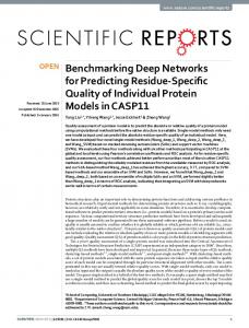
2015). CNNs are promising for financial predictions based on time series data for two main reasons: First, high level features abstracted by the network may serve the purpose that noise filters and dimensionality reduction techniques play in successful prediction models that use carefully crafted input features. Secondly, the temporally-local correlation between consecutive observations can be exploited to reduce the number of parameters to be estimated in the network by connecting only a small number of adjacent inputs to each unit in a hidden layer. Units in a CNN receive inputs from small contiguous sub-regions of the input space, called a receptive field that collectively cover the entire set of input features. This allows units to act as local filters and to exploit local correlation between contiguous inputs. Figure 1 shows three layers of a CNN where units in each layer are connected to only 3 adjacent units from the previous layer and thus have receptive fields of width 3. Notice, though, that the unit in layer h+1 is indirectly responsive to all 5 units in layer h-1. Units share weights and bias parameters to create a feature map; this results in a significant reduction in the number of parameters to be estimated and facilitates detection of features irrespective of their actual position in the input field. In figure 1 the red, green, and blue connections in each layer share the same weights. Thus only three weights connecting layer h-1 to layer h need to be estimated compared to 15 weights in a conventional network where all 5 inputs are connected to every unit in the next layer. This reduction in the number of parameters may be very significant as the number layers in the network and the number of units in each layer increases.

Figure 1. Local connectivity in a deep convolution neural network.

6

Svitlana Galeshchuk, Sumitra Mukherjee

The output of each unit in a convolution layer is obtained by applying a non-linear function – typically a rectified linear unit (ReLU) – to the dot product of its input vector and the corresponding weight vector; ReLU simply returns output max⁡(0, 𝑧) for an input 𝑧. Figure 2 shows the architecture of a CNN with several convolution layers interspersed with pooling layers. Pooling partitions the input space into disjoint sub-regions and returns the maximum value in the sub-region. This reduces the computational costs in the upper layers and provides translational invariance. The final layer is fully connected with a softmax function applied to the weighted sum of the inputs.

Figure 2. Architecture of a deep convolution neural network.

Langkvist et al (2014) provide a good review of deep learning for time-series modeling. Details of the CNN architecture in our study are presented in the methodology section. 3. Methodology We first describe the data sets used in this study. Next, we discuss baseline models including shallow neural network and support vector machines that are trained as classifiers using derived input features. Finally, the deep convolution neural network is explained. 3.1. Data used and evaluation measure We use the daily closing rates between three currency pairs: Euro and US Dollar (EUR/USD), British Pound and US Dollar (GBP/USD), and US Dollar and Japanese Yen (USD/JPY) to train and test our models; these are among the most traded currency pairs in 7

Svitlana Galeshchuk, Sumitra Mukherjee

the forex market. The rates are publicly available and may be downloaded from: http://www.global-view.com/forex-trading-tools/forex-history/. We use 3 different time series data sets, one for each currency pair: EUR/USD, GBP/USD, and USD/JPY. Figure 3. plots the data. Each data set has 1565 observations (representing 1565 daily closing rates for the years 2010 to 2015).

8

Svitlana Galeshchuk, Sumitra Mukherjee

Figure 3. Foreign exchange data used in the study. For each data set we predict the direction of change 𝑘 periods forward, with 𝑘 ranging from 1 to 30; we refer to each 𝑘 period forward classification problem as a “problem instance”. For each problem instance, the first 1043 observations (daily closing rates for the years 2010 to 2013) are used to train our models and the last 522 observations (daily closing rates for the years 2014 and 2015) are used to test the trained models. Thus two-thirds of our observations are used for training and the remaining one-third are used for testing. Note that for a 𝑘 period forward prediction problem the true directions of change are not available for the last 𝑘 test samples. 3.2. Baseline Models We use a naïve method, two time series models (ARIMA and ETS), and a single layered neural network as baseline models. The naïve method predicts the majority class in the training set as the output for any test example. That is, the class of a test example is predicted as 1 if the exchange rate increases in at least 50% of the training examples and predicted as 0 otherwise. We call this model MC (Majority Class). The purpose of this model is to check whether classification accuracy is simply an artifact of similar overall trends in the training and test data. The time series models (ARIMA and ETS) provide point estimates 𝑦̂𝑡+𝑘 for the rates. We predict output class 𝑧̂𝑘 (𝑡) = 1 if 𝑦̂𝑡+𝑘 > 𝑦𝑡 , and 0 otherwise. The predicted direction of change 𝑧̂𝑘 (𝑡) is compared with the actual direction of change 𝑧𝑘 (𝑡). Results for ARIMA and ETS are obtained using the auto.arima model and the ets model from the R library forecast with default parameters (Hyndman and Khandakar 2008). The neural network model (ANN) has a single hidden layer. After tuning the parameters of the network, best results on out-of-sample data were obtained using 10 hidden neurons. The units have sigmoid transfer functions and use gradient descent and backpropagation for training. The model is trained on vectors with 𝑝 features (𝑦𝑡 , 𝑦𝑡−1 , … , 𝑦𝑡−𝑝+1 ) as inputs and 𝑦𝑡+𝑘 as output to predict a point estimate 𝑦̂𝑡+𝑘 for the 𝑘 period forward rate. As in the case of the time series models, we predict the output class 𝑧̂𝑘 (𝑡) = 1 if 9

Svitlana Galeshchuk, Sumitra Mukherjee

𝑦̂𝑡+𝑘 > 𝑦𝑡 , and 0 otherwise to compare the actual and predicted directions of change. Results

are

obtained

using

the

R

package

nnet

(https://cran.r-project.org/web/packages/nnet/nnet.pdf). Models parameters were obtained using

the

tune

function

from

the

R

package

e1071

(https://cran.r-project.org/web/packages/e1071/e1071.pdf) that tunes hyperparameters of the model through cross-validation by performing a grid search over the parameter ranges. 3.3. Machine learning classifiers with derived features The baseline models are trained to provide point estimates while our goal is to predict the direction of change. For a fair comparison with our deep networks that are trained as classifiers, we also trained neural network models and support vector machines (SVM) as classifiers using the true direction of change 𝑧𝑘 (𝑡) as output labels for each 𝑘 period forward problem instance. To further improve classification accuracy, these models were trained with derived input features; moving averages were used as input features since they are commonly used in the financial because of their ability to filter out random noise(Lukas 2007) . We refer to the artificial neural network model trained on moving averages as input features as ANNMA to distinguish it from the artificial neural network model ANN that is trained on raw time series data as input features. ANNMA uses a single hidden layer with 10 units. The hidden units use sigmoid transfer functions while the output unit uses a sofmax transfer function. Models were trained using the R package nnet with gradient descent and backpropagation used for learning. The SVM models were trained using the R package svm from the e1071 library (https://cran.r-project.org/web/packages/e1071/vignettes/svmdoc.pdf) using polynomial kernels. We also ran experiments using linear and radial basis kernels, but the classification accuracies obtained these kernel functions were significantly lower than those obtained with the polynomial kernel. For both, ANNMA and SVM, the tune function from the R package e1071 was used to obtain best hyperparameters values through cross-validation. 3.4. Deep Networks 10

Svitlana Galeshchuk, Sumitra Mukherjee

Our deep convolution neural network (CNN) has 𝑙 layers of hidden units separating the input layer from the output unit. We use 𝑏𝑗𝑖 to denote the internal bias of the 𝑗th unit in the 𝑖 th layer and 𝑊𝑗𝑘𝑖 to represent the weight of the connection to that unit from the 𝑘th unit in the (𝑖 − 1)th layer. For an input vector 𝒙, the output of 𝑗th unit in the 𝑖 th layer is computed as ℎ𝑗𝑖 (𝒙) = 𝑅𝑒𝐿𝑈(𝑎𝑗𝑖 ), where 𝑎𝑗𝑖 = 𝑏𝑗𝑖 + ∑𝑘 𝑊𝑗𝑘𝑖 ℎ𝑘𝑖−1 (𝒙), and 𝑅𝑒𝐿𝑈(𝑎) = max⁡(0, 𝑎) is the rectified linear unit function. The output uses a softmax transfer function. Adam optimizer (Kigma et al 2015) is used to minimize a cross-entropy loss function. The open source library TensorFlow (https://www.tensorflow.org/) was used to create the CNN models. Ten-fold cross-validation was used to decide on parameter values. Results are reported with out-of-sample data using a network with 4 hidden layers with the following parameters: width = 5, height = 1, depth = 1, stride = 2, and padding=0. 4. Results Table 1 presents the mean of the absolute prediction error of the point estimates expressed as a percentage of the true value by ARIMA, ETS, and ANN for the three currency pairs. The only purpose of presenting these results is to illustrate that although these baseline models result in relatively low absolute errors for point estimates, they are poor at predicting the direction of change (see tables 2, 3, and 4). The absolute percentage error for a 𝑘-period for𝑦𝑡+𝑘 −𝑦̂𝑡+𝑘

ward prediction in period 𝑡 is given by as |

𝑦𝑡+𝑘

| ×100. The methods are very similar

in terms of the absolute percentage error of their point estimates. The errors are less than 2.4% in all instances, suggesting that these models provide satisfactory point estimates. With ANN, ANNMA, SVM, and CNN, we ran preliminary experiments with the number of input features 𝑝 ranging from 5 to 50. Classification accuracy across models was somewhat lower with 𝑝 < 20, but did not improve with 𝑝 > 30. In this paper we present results with 𝑝=30, but results are qualitatively similar for 𝑝 ranging between 25 and 30. Thus we use the rates from 30 previous periods as inputs since we predict rates up to 30 periods forward. For the classifiers ANNMA and SVM, we use fifth order moving averages rather than the closing rates as derived input features. Experiments were run with moving average orders ranging from 2 to 10 to settle upon moving averages of order 5 as the one that produced the best results in a plurality of problem instances. 11

Svitlana Galeshchuk, Sumitra Mukherjee

12

Svitlana Galeshchuk, Sumitra Mukherjee

Table 1. Mean absolute percentage error in predicted point estimates by baseline models. k 1 2 3 4 5 6 7 8 9 10 11 12 13 14 15 16 17 18 19 20 21 22 23 24 25 26 27 28 29 30

EUR/USD GBP/USD ARIMA ETS ANN ARIMA ETS 0.3% 0.3% 0.3% 0.3% 0.3% 0.4% 0.4% 0.4% 0.4% 0.4% 0.5% 0.5% 0.5% 0.5% 0.5% 0.5% 0.5% 0.5% 0.5% 0.5% 0.6% 0.6% 0.6% 0.6% 0.6% 0.7% 0.7% 0.7% 0.7% 0.7% 0.7% 0.7% 0.7% 0.7% 0.7% 0.7% 0.7% 0.7% 0.7% 0.7% 0.8% 0.8% 0.8% 0.8% 0.8% 0.8% 0.8% 0.8% 0.8% 0.8% 0.9% 0.9% 0.9% 0.9% 0.9% 0.9% 0.9% 0.9% 0.9% 0.9% 1.0% 1.0% 1.0% 0.9% 0.9% 1.0% 1.0% 1.0% 1.0% 1.0% 1.0% 1.1% 1.1% 1.0% 1.0% 1.1% 1.1% 1.1% 1.1% 1.1% 1.1% 1.1% 1.1% 1.1% 1.1% 1.1% 1.2% 1.1% 1.2% 1.2% 1.2% 1.2% 1.2% 1.2% 1.2% 1.2% 1.3% 1.2% 1.3% 1.3% 1.3% 1.3% 1.3% 1.3% 1.3% 1.3% 1.4% 1.3% 1.4% 1.4% 1.3% 1.4% 1.4% 1.4% 1.4% 1.4% 1.5% 1.4% 1.5% 1.5% 1.4% 1.5% 1.5% 1.5% 1.5% 1.5% 1.6% 1.5% 1.5% 1.5% 1.5% 1.6% 1.6% 1.6% 1.6% 1.5% 1.6% 1.6% 1.6% 1.6% 1.6% 1.7% 1.6% 1.7% 1.6% 1.6% 1.7% 1.7% 1.7% 1.7%

USD/JPY ANN ARIMA ETS ANN 0.3% 0.3% 0.3% 0.3% 0.4% 0.5% 0.5% 0.5% 0.5% 0.6% 0.6% 0.6% 0.5% 0.8% 0.8% 0.8% 0.6% 0.9% 0.9% 0.9% 0.7% 1.0% 1.0% 1.0% 0.7% 1.0% 1.0% 1.0% 0.7% 1.1% 1.1% 1.1% 0.8% 1.1% 1.2% 1.1% 0.8% 1.2% 1.2% 1.2% 0.9% 1.3% 1.3% 1.3% 0.9% 1.4% 1.4% 1.4% 0.9% 1.5% 1.4% 1.5% 1.0% 1.6% 1.5% 1.6% 1.0% 1.7% 1.6% 1.6% 1.1% 1.7% 1.6% 1.7% 1.1% 1.8% 1.7% 1.7% 1.2% 1.8% 1.7% 1.8% 1.2% 1.9% 1.8% 1.8% 1.3% 2.0% 1.8% 1.9% 1.3% 2.0% 1.9% 2.0% 1.4% 2.1% 2.0% 2.1% 1.4% 2.2% 2.1% 2.1% 1.5% 2.2% 2.1% 2.2% 1.5% 2.2% 2.2% 2.2% 1.5% 2.3% 2.2% 2.2% 1.6% 2.3% 2.2% 2.2% 1.6% 2.2% 2.3% 2.3% 1.6% 2.3% 2.3% 2.3% 1.7% 2.3% 2.4% 2.3%

13

Svitlana Galeshchuk, Sumitra Mukherjee

Figure 4 presents the out of sample classification accuracy obtained by the baseline models (MC, ARIMA, ETS, and ANN), the classifiers (ANNMA, and SVM), and the deep network (CNN) for forex rates EUR/USD, GBP/USD, and USD/JPY, respectively. Results are displayed for a 𝑘 period forward prediction problem with 𝑘 ranging from 1 to 30 along the horizontal axis. Tables 2, 3, and 4 present the same out-of-sample classification accuracies expressed as percentages rounded to the second decimal place. Recall that classification accuracy is measured as the percentage of test samples for which the direction of change is predicted accurately. The classification accuracy for the baseline models (MC, ARIMA, ETS, and NN) that provide point estimates using raw time series data as input features vary roughly between 40% and 60%, indicating that they are not significantly different from random guesses. The classifiers ANNMA and SVM that are trained using derived features (moving averages) as inputs and actual class labels for the direction of change do somewhat better with classification accuracies around 65%. Our deep convolution neural networks result in average classification accuracies over 75%. Table 5 presents results for paired two sample tests for means where the classification accuracy of CNN is compared to the best performing alternate classifier. That is, the highest classification accuracy obtained using any of the other models – MC, ARIMA, ETS, NN, ANNMA, or SVM – is compared to the classification accuracy produced by CNN. The sample size with each data set is 30, resulting from the 𝑘-period forward classification problem instances with 𝑘 ranging from 1 to 30. T-test results are presented with 𝛼 = 0.001. The null hypothesis that the mean classification accuracy of CNN is equal to the mean classification accuracy of the best of the alternate classifiers is rejected in favor of the alternate hypothesis that CNN results in a higher classification accuracy for all three exchange rate considered.

14

Svitlana Galeshchuk, Sumitra Mukherjee

Figure 4. Comparison of classification accuracy on out-of-sample data 15

Svitlana Galeshchuk, Sumitra Mukherjee

Table 2. Classification accuracy for EUR/USD. k 1 2 3 4 5 6 7 8 9 10 11 12 13 14 15 16 17 18 19 20 21 22 23 24 25 26 27 28 29 30 Mean min Q1 Median Q3 max

MC ARIMA ETS ANN ANNMA SVM CNN 47.92% 55.91% 58.93% 55.27% 60.81% 60.57% 78.53% 46.16% 53.53% 50.44% 64.37% 64.86% 65.43% 81.73% 41.04% 55.25% 52.94% 71.83% 73.19% 73.81% 89.55% 37.65% 56.94% 53.05% 70.30% 71.93% 70.54% 73.28% 64.09% 56.00% 43.93% 66.97% 68.44% 67.78% 71.65% 38.02% 57.28% 50.36% 68.89% 69.85% 69.63% 74.42% 32.49% 58.98% 50.19% 70.59% 71.30% 71.97% 88.21% 32.23% 61.42% 54.97% 60.89% 63.00% 62.66% 70.35% 29.88% 58.05% 50.05% 58.01% 59.12% 59.08% 73.67% 31.20% 58.21% 48.40% 57.26% 59.87% 59.02% 67.83% 29.53% 62.45% 53.10% 66.90% 67.76% 68.87% 78.36% 30.86% 51.69% 53.49% 59.04% 63.61% 62.20% 73.31% 33.67% 60.04% 57.28% 55.67% 60.87% 60.29% 73.67% 31.50% 61.77% 53.87% 54.29% 63.70% 62.33% 62.61% 32.71% 61.74% 55.09% 58.93% 62.30% 63.32% 71.35% 35.10% 58.83% 54.44% 56.32% 59.35% 59.46% 64.10% 31.28% 60.91% 55.90% 55.90% 62.57% 62.28% 73.89% 28.97% 60.94% 51.60% 53.93% 62.75% 61.52% 65.41% 29.16% 63.08% 50.95% 52.14% 63.49% 64.67% 73.46% 29.23% 62.62% 49.58% 53.55% 62.76% 63.09% 77.54% 26.19% 63.18% 50.52% 49.65% 63.70% 64.69% 71.51% 23.93% 64.38% 54.54% 50.20% 64.70% 66.17% 75.04% 26.11% 62.50% 53.21% 52.65% 64.42% 63.30% 73.75% 71.05% 61.69% 52.91% 56.20% 64.22% 62.74% 77.87% 70.81% 60.30% 50.24% 62.41% 71.45% 70.84% 84.06% 25.37% 62.81% 50.51% 54.24% 63.26% 63.98% 69.24% 23.80% 61.24% 51.06% 49.79% 62.35% 61.54% 78.41% 75.87% 63.63% 49.54% 54.89% 76.83% 76.06% 83.56% 76.80% 61.94% 51.37% 57.39% 67.16% 65.05% 80.60% 76.37% 64.17% 48.93% 51.47% 72.36% 71.02% 81.51% 40.30% 60.05% 52.05% 58.33% 65.40% 65.13% 75.28% 23.80% 51.69% 43.93% 49.65% 59.12% 59.02% 62.61% 29.31% 58.09% 50.27% 54.01% 62.62% 62.22% 71.55% 32.36% 61.09% 51.49% 56.26% 63.70% 63.65% 73.82% 44.88% 62.49% 53.77% 62.03% 68.27% 68.60% 78.50% 76.80% 64.38% 58.93% 71.83% 76.83% 76.06% 89.55%

16

Svitlana Galeshchuk, Sumitra Mukherjee

Table 3. Classification accuracy for GBP/USD. k 1 2 3 4 5 6 7 8 9 10 11 12 13 14 15 16 17 18 19 20 21 22 23 24 25 26 27 28 29 30 Mean min Q1 Median Q3 max

MC 50.71% 46.02% 45.95% 45.68% 43.56% 43.96% 40.44% 40.64% 40.09% 40.40% 38.60% 39.97% 36.95% 36.70% 39.19% 40.14% 37.96% 40.42% 40.11% 40.31% 39.97% 39.30% 40.51% 36.60% 37.12% 41.14% 39.29% 42.04% 41.26% 41.52% 40.88% 36.60% 39.29% 40.35% 41.45% 50.71%

ARIMA 47.62% 45.27% 49.35% 50.64% 51.77% 48.56% 50.48% 51.47% 51.42% 47.08% 51.70% 51.33% 50.71% 51.01% 48.90% 51.09% 53.53% 52.42% 55.68% 56.63% 53.21% 55.65% 56.33% 56.56% 57.32% 56.20% 55.55% 57.30% 57.39% 56.73% 52.63% 45.27% 50.66% 51.74% 56.07% 57.39%

ETS 48.74% 49.85% 48.18% 53.16% 47.02% 49.49% 51.54% 50.73% 47.56% 48.56% 48.62% 52.64% 53.55% 49.12% 46.53% 48.40% 47.65% 48.49% 48.81% 49.39% 48.82% 48.62% 49.01% 48.01% 46.52% 46.79% 48.41% 45.41% 50.34% 50.73% 49.02% 45.41% 48.05% 48.68% 49.76% 53.55%

ANN ANNMA SVM CNN 49.78% 52.60% 51.73% 56.29% 68.99% 73.04% 70.50% 77.81% 62.18% 71.49% 69.71% 75.39% 64.44% 71.22% 69.04% 76.55% 70.79% 75.16% 71.84% 79.31% 71.17% 69.88% 71.06% 80.01% 71.58% 74.93% 73.87% 72.49% 65.56% 66.67% 69.04% 74.24% 69.08% 74.40% 70.32% 77.66% 64.32% 68.83% 64.61% 74.72% 62.85% 65.75% 65.72% 73.48% 69.03% 71.72% 71.05% 81.80% 61.39% 64.80% 63.87% 79.59% 58.82% 60.05% 59.52% 73.60% 59.95% 64.20% 62.11% 63.79% 55.49% 56.78% 57.48% 68.30% 58.93% 61.80% 59.51% 72.65% 63.20% 68.36% 66.12% 76.77% 60.19% 62.44% 61.31% 78.41% 64.46% 68.06% 68.14% 75.35% 65.53% 69.65% 67.70% 78.61% 62.79% 64.33% 62.95% 68.81% 59.14% 63.22% 59.84% 69.30% 55.54% 59.59% 57.67% 69.43% 61.84% 65.70% 62.57% 70.48% 57.28% 63.05% 59.72% 70.48% 64.83% 68.43% 65.76% 74.86% 57.02% 60.18% 61.26% 71.12% 58.29% 63.33% 59.28% 67.92% 64.08% 67.36% 65.47% 83.72% 62.62% 66.23% 64.63% 73.77% 49.78% 52.60% 51.73% 56.29% 58.98% 63.10% 60.19% 70.48% 62.82% 66.21% 65.04% 74.48% 65.36% 69.82% 69.04% 77.77% 71.58% 75.16% 73.87% 83.72%

17

Svitlana Galeshchuk, Sumitra Mukherjee

Table 4. Classification accuracy for USD/JPY. k 1 2 3 4 5 6 7 8 9 10 11 12 13 14 15 16 17 18 19 20 21 22 23 24 25 26 27 28 29 30 Mean min Q1 Median Q3 max

MC 41.13% 43.47% 46.93% 54.88% 45.50% 39.78% 40.93% 42.90% 42.36% 45.26% 43.57% 56.00% 44.45% 41.08% 43.18% 42.25% 63.11% 62.82% 60.03% 63.75% 59.37% 40.25% 40.04% 38.11% 37.56% 37.11% 37.76% 32.29% 34.09% 34.53% 45.15% 32.29% 39.84% 42.63% 46.57% 63.75%

ARIMA 49.80% 48.97% 51.63% 48.79% 44.98% 44.56% 45.18% 43.43% 47.42% 48.90% 48.63% 47.71% 47.89% 42.52% 44.83% 47.28% 46.64% 47.64% 51.49% 49.80% 49.87% 48.59% 44.98% 45.51% 44.23% 47.63% 49.93% 50.54% 51.79% 50.70% 47.73% 42.52% 45.26% 47.80% 49.80% 51.79%

ETS 44.57% 50.24% 45.77% 47.69% 52.17% 51.94% 54.52% 50.20% 51.90% 49.12% 48.77% 52.96% 49.66% 49.53% 49.74% 53.22% 52.54% 51.29% 49.70% 45.33% 46.99% 46.44% 51.17% 55.19% 52.79% 55.77% 53.66% 52.43% 45.80% 47.17% 50.28% 44.57% 47.96% 50.22% 52.52% 55.77%

ANN ANNMA SVM CNN 39.82% 48.80% 47.07% 57.03% 68.00% 73.65% 70.86% 80.64% 63.06% 71.76% 74.84% 86.90% 69.23% 73.09% 71.66% 87.74% 69.71% 71.01% 69.44% 86.05% 62.20% 64.16% 67.04% 79.25% 64.34% 75.51% 66.91% 85.71% 65.86% 69.78% 65.99% 73.27% 69.56% 71.65% 73.13% 92.62% 62.87% 63.82% 62.95% 69.86% 68.09% 70.44% 68.81% 84.39% 61.40% 68.37% 65.77% 77.96% 60.89% 64.90% 67.44% 76.82% 60.31% 63.79% 64.46% 83.47% 59.30% 62.29% 65.75% 69.42% 62.46% 66.72% 62.04% 77.44% 61.49% 64.62% 65.38% 77.17% 59.72% 64.29% 61.02% 86.01% 68.42% 67.62% 68.95% 83.38% 66.75% 69.88% 68.40% 86.60% 57.29% 56.81% 58.51% 79.19% 53.93% 59.61% 58.67% 74.28% 60.87% 65.27% 63.35% 72.58% 57.00% 60.74% 60.17% 78.04% 59.84% 64.51% 62.75% 84.90% 63.70% 68.85% 63.54% 84.65% 63.18% 63.97% 63.36% 81.58% 53.86% 56.55% 59.21% 65.93% 56.76% 63.40% 60.01% 77.26% 59.83% 62.81% 66.36% 78.05% 61.66% 65.62% 64.80% 79.27% 39.82% 48.80% 47.07% 57.03% 59.75% 63.50% 62.21% 76.91% 61.84% 64.76% 65.57% 79.22% 65.48% 69.85% 68.16% 84.84% 69.71% 75.51% 74.84% 92.62%

18

Svitlana Galeshchuk, Sumitra Mukherjee

Table 5. Paired two sample test for mean classification accuracy: CNN vs best alternate. t statistics P(T