Deep neural networks for direct, featureless learning through observation: the case of 2d spin models K. Mills∗ Dept. of Physics, University of Ontario Institute of Technology
I. Tamblyn†
arXiv:1706.09779v1 [cond-mat.mtrl-sci] 29 Jun 2017
Dept. of Physics, University of Ontario Institute of Technology, University of Ottawa & National Research Council of Canada (Dated: June 30, 2017) We train a deep convolutional neural network to accurately predict the energies and magnetizations of Ising model configurations, using both the traditional nearest-neighbour Hamiltonian, as well as a long-range screened Coulomb Hamiltonian. We demonstrate the capability of a convolutional deep neural network in predicting the nearest-neighbour energy of the 4 × 4 Ising model. Using its success at this task, we motivate the study of the larger 8 × 8 Ising model, showing that the deep neural network can learn the nearest-neighbour Ising Hamiltonian after only seeing a vanishingly small fraction of configuration space. Additionally, we show that the neural network has learned both the energy and magnetization operators with sufficient accuracy to replicate the low-temperature Ising phase transition. Finally, we teach the convolutional deep neural network to accurately predict a long-range interaction through a screened Coulomb Hamiltonian. In this case, the benefits of the neural network become apparent; it is able to make predictions with a high degree of accuracy, 1600 times faster than a CUDA-optimized “exact” calculation.
INTRODUCTION
The collective behaviour of interacting particles, whether electrons, atoms, or magnetic moments, is the core of condensed matter physics. The difficulties associated with modelling such systems arise due to the enormous number of free parameters defining a nearinfinite configuration space for systems of many particles. In these situations, where exact treatment is impossible, machine learning methods have been used to build better approximations and gain useful insight. This includes the areas of dynamical mean-field theory, strongly correlated materials, phase classification, and materials exploration and design [1–8]. As an introductory many-particle system, one is commonly presented with the square two-dimensional Ising model, a ubiquitous example of a ferromagnetic system of particles. The model consists of an L × L grid of discrete interacting “particles” which either possess a spin up (σ = 1) or spin down (σ = −1) moment. The internal energy associated with a given configuration of spins ˆ = −J P σi σj where the is given by the Hamiltonian H sum is computed over all nearest-neighbour pairs (hi, ji), and J is the interaction strength. For J = 1, the system behaves ferromagnetically; there is an energetic cost of having opposing neighbouring spins, and neighbouring aligned spins are energetically favourable. The canonical Ising model defined on an infinite domain (i.e. periodic boundary conditions) is an example of a simple system which exhibits a well-understood continuous phase transition at a critical temperature Tc ≈ 2.269. At temperatures below the critical temperature, the system exhibits highly ordered behaviour,
with most of the spins in the system aligned. Above the critical temperature, the system exhibits disorder, with, on average roughly equivalent numbers of spin up and spin down particles. The “disorder” in the system can be represented by an order parameter known as the “magnetization” M , which is merely the average of all L2 individual spins. Configurations of the Ising model can be thought to belong to one of two phases. Artificial neural networks have been shown to differentiate between the phases [9, 10], effectively discovering phase transitions. This is, however, merely a binary classification problem based on the magnetization order parameter. The membership of a configuration to either the high- or low-energy class does not depend upon any interaction between particles within the configuration. Furthermore, convolutional neural networks have been trained to estimate critical parameters of Ising systems [11]. Machine learning methods have been demonstrated previously in many-body physics applications [6] and other two-dimensional topological models are discussed frequently [12, 13] in quantum field theory research. However, the use of deep convolutional neural networks remains infrequent, despite their recently presented parallels to renormalization group [14] and their frequent successes in difficult machine learning and computer vision tasks, some occurring a decade ahead of expectations [15, 16]. We demonstrate that a convolutional deep neural network, trained on a sufficient number of examples, can take the place of conventional operators. Traditional machine learning techniques depend upon the selection of a set of descriptors (features) [17]. Convolutional deep neural networks have the ability to establish a set of rel-
2 evant features without human intervention, by exploiting the spatial structure of input data (e.g. images, arrays). Without human bias, they detect and optimize a set of features, and ultimately map this feature set to a quantity of interest. For this reason, we choose to call deep convolutional neural networks “featureless learning”. Furthermore, we demonstrate that a neural network trained in this way can be practically applied in a simulation to accurately compute the temperature dependence of the heat capacity. In doing so, we observe its peak at the critical temperature, a well-understood [18] indication of the Ising phase transition.
METHODS Deep learning
We used a very simple deep neural network architecture, shown in Fig. 1. In previous work, we demonstrated that the same neural network structure, differing only in the number of repeat units, was capable of predicting quantities associated with the one-electron Schr¨odinger equation [19]. In this network, the convolutional layers work by successively mapping an image into a feature space where interpolation is possible using a nonlinear boundary. The final decision layers impose this boundary and produce an output value. A detailed overview of the network, training procedure, and data acquisition is presented in the Supplementary Information.
FIG. 1. Deep neural network architecture used for predicting Ising model operators. The network consists of 7 convolutional layers with two fully-connected layers at the top. On the left, the output of a given filter path is shown for an example Ising configuration. The final 2 × 2 output is fed into a wide fully-connected layer. ReLU (recified linear unit) activation is used on all convolutional layers.
2 10 3
RESULTS
We begin our investigation with the 4 × 4 Ising model, as the configuration space is of a manageable size that we can easily compute all possible configurations (65536 total unique configurations). Because of this, we can explicitly evaluate how well a model performs by evaluating the model on the entirety of configuration space. The energies of these configurations are discrete, taking on 15 possible values (for the 4×4 model) ranging from −32J to 32J. The discrete energy values allow us to treat energy prediction as a machine learning “classification problem”. In the areas of handwriting recognition and image classification, deep convolutional neural networks with such an output structure have excelled time and time again [20–23]. We generated three independent datasets, each consisting of 27,000 training examples (1800 examples per class), gathered in an intelligent way to sample across the entire range of energies (more information in the Supplementary Information). Each dataset contains less than 20% of configuration space. We trained our neural network
Energy per site
The 4 × 4 Ising model
1 10 2
0
10 1
1
2 1.0
0.5 0.0 0.5 Magnetization per site
1.0
10 0
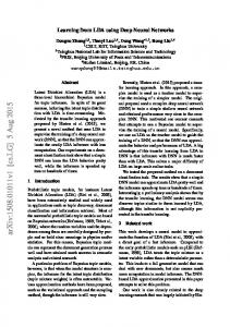
FIG. 2. Configuration space of the 4 × 4 Ising model. The colors represent the density of states.
architecture on each of these three datasets. The neural network was able to classify all but a handful of Ising configurations, on average. On one dataset, it achieved an accuracy of 100%. In all cases of misclassification, 100% of misclassified examples only have an error of ±1 energy level, indicating the neural network is just barely failing to classify such examples. All misclassified configurations had energies near zero. In this region there is considerable variation due to the degeneracy of the Ising
3 model (apparent in Fig. 2), and therefore predictions based on a uniform number of training examples per class are slightly more challenging. At the extremes energies (±32), individual configurations are repeated many times in order to fill the quota of training examples. It is worth noting again that this neural network had access to less than 20% of configuration space so it is clearly correctly inferring information about examples it has not yet seen.
The 8 × 8 Ising model
Although the 4 × 4 model is instructive, larger Ising models such as the 8 × 8 model are interesting since the 2 enormity of configuration space (28 ≈ 1019 ) precludes training on even a modest fraction of possible configurations, so the neural network truly needs to “learn” how to predict energies from seeing only a minuscule fraction of configuration space. The neural network achieves 99.922% accuracy, almost perfect performance, with a training dataset of 100,000 configurations, a vanishingly small subset of configuration space. Note that we can no longer report an accuracy computed over the entirety of configuration space, so we must report the accuracy of the model on a separate testing set of data. The testing dataset consists of 50,000 examples separated from the training dataset prior to training. No examples in the testing set appear in the training set. Importantly, as with the 4 × 4 model, in the few cases where the model did fail, it did not fail by very much: 100% of the time, the predicted class is either correct or only one energy class away from correct. The neural network does exceptionally well at predicting energies when only exposed to a small subset of configuration space during training.
Regression
In practice, a deep neural network capable of classifying configurations into well-defined bins is less appealing than one which could predict continuous variables. “Real-life” systems rarely exhibit observables and characteristics that are quantized at the scales relevant to the big-picture problem. The total energy of atomic configurations, vibrational frequencies, bond lengths, etc. all admit a continuum of values. As such, this is a good opportunity to investigate a form of deep neural network output structure known as “regression”. In a regression network, insead of the final fully connected layer having a width equal to the number of classes, we use a fully connected layer of width 1: a single output value. In this case, a softmax cross-entropy loss layer is no longer appropriate. The simplest form of loss function for a single-output regression network is the mean-squared error between network predictions and the true value of the
energy. We modify the deep neural network in this way to perform regression. Changing nothing about the training process other than the loss function, we see that the model performs quite well, with a median absolute error of 1.782J. With the Ising model, the allowed energy classes are separated by 4 energy units, so an error of 1.782J is consistent with the capability of the network to accurately classify examples into these bins of width 4. Additionally, we trained the deep neural network to learn the magnetization; it performs exceptionally well with a median absolute error of 4 × 10⁻³ per spin and 2 × 10⁻³ per spin for the 4 × 4 and 8 × 8 models, respectively. This is not particularly surprising as the magnetization is a very simple, non-interacting operator. This effectively amounts to using a convolutional neural network to compute the sum of an array; we present it merely as a demonstration of a neural network’s ability to learn multiple mappings.
Replicating the Ising Model phase transition
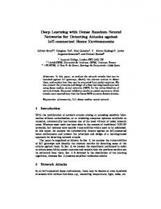
The Ising model defined on an infinite domain exhibits a phase transition at a critical temperature Tc ≈ 2.269. For a finite domain under periodic boundary conditions, however, a correction factor γ is necessary to compensate for the correlations between periodic lattice images. This behaviour is discussed in detail in Ferdinand and Fisher’s 1969 work (ref. [18]), and in this analysis we will denote the “theoretical” critical temperature as γTc . Using a Metropolis-Hastings algorithm, one can sample the configuration space accessible to the Ising model at a given temperature. Using a Boltzmann rejection ¯ can be computed probability, the mean energy per site, E for a given temperature. Repeating for various temper¯ against T and observe the atures allows one to plot E phase transition. The Metropolis-Hastings algorithm, and thus the demonstration of this phase transition depends on the accurate evaluation of Ising configuration energies. We generated the phase diagram for the 4 × 4 Ising model, evaluating the energy using the exact Hamiltonian. Then, we replaced the magnetization and energy operators with the trained deep neural networks. The phase diagrams match exactly, and are presented in Figs. 3 and 4. We repeated this exercise with the 8 × 8 classification model and observe the phase transition. Again, the deep neural network had learned the energy and magnetization operators with sufficient precision to replicate the phase transition, shown in Fig. 5.
4
0.5
Long-range interactions
1.0
¯ 2 E/n
0.8
Specific heat, C
¯ 2 Mean energy per site, E/n
1.2
1.0
0.6 1.5
0.4
1 E¯
C = n2
γ Tc
2.0 1
2
3 4 Temperature, T [kB ]
0.2
T
5
6
0.0
Mean absolute magnetization, M¯
FIG. 3. The average energy per site at various temperatures, as well as the heat capacity, C for the 4 × 4 Ising model. The solid lines and dots indicate the energy evaluation methods used: the exact Hamiltonian, and DNN, respectively. These results are averaged over 400 independent simulations. The standard deviation is negligibly small.
exact DNN, targeted sampling
1.0 0.8 0.6 0.4
γ Tc
0.2 0.0 1
2
3 4 Temperature, T [kB ]
5
6
FIG. 4. The magnetization per site at various temperatures for the 4 × 4 Ising model. The solid line denotes the simulation using the exact magnetization and energy operators, and the dots represent the deep-learned energy and magnetization operators. These results are averaged over 400 independent simulations. The standard deviation is negligibly small.
0.5
0.8
1.0
0.6 1.5
0.4
γ Tc
2.0 1
2
3 4 Temperature, T [kB ]
1 E¯
C = n2 5
Discussion
1.0
¯ 2 E/n
Specific heat, C
¯ 2 Mean energy per site, E/n
1.2
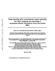
The traditional Ising Hamiltonian is a very short-range interation, including only nearest-neighbour interactions. Physical systems frequently depend on long-range interations. Herein, we demonstrate that the same deep neural network is able to learn the energies associated with a screened Coulomb Hamiltonian: the traditional pairwise Coulomb interation attenuated by an exponential term [24, 25]. We computed this energy for 120,000 8 × 8 Ising configurations using an explicit sum method and periodic boundary conditions, ensuring the infinite summation was converged sufficiently for the effective cutoff we used of 64 units, i.e. 8 times the size of the unit lattice. The summation is very computationally expensive, as it must be computed for every pair of spins between the unit lattice and all periodic images until the effective cutoff radius is reached and the sum converges. Since the algorithm is amenable to parallelization, we implemented it in CUDA for performance [26]. We trained our deep neural network on a set of 100,000 examples, and tested the network on a non-intersecting set of 20,000 examples. Our neural network is able to learn the Hamiltonian with considerable accuracy, performing with a median absolute error of 0.640J energy units. The performance of the model is shown in Fig. 6. While the accurate learning of the long-range interaction is in itself impressive, additionally the deep neural network drastically outperforms the explicit calculation in terms of speed. The deep neural network can make predictions at a rate 1600 times faster than the CUDA-enabled “exact” calculation (performing at comparable median error), when running on a single NVIDIA Tesla K40.
0.2
T
6
0.0
FIG. 5. The average energy per site at various temperatures, as well as the heat capacity for the 8 × 8 Ising model. The solid line denotes the simulation using the exact Hamiltonian, and the dots represent the deep-learned Hamiltonian. These results are averaged over 400 independent simulations. The standard deviation is negligibly small.
A question one may ask is whether deep neural networks are the right tool for the job. Certainly, there are other machine learning methods which do not involve such an expensive training process as deep neural networks demand. In addition to a deep convolutional neural network, we tried two other commonly-used machine learning algorithms, kernel ridge regression (KRR) and random forests (RF), on various dataset sizes. For the 8 × 8 regression model, KRR performed at best poorly with a median absolute error of 60.3J. RF performed much better than KRR with a MAE of 5.8J (still far inferior to the deep neural network). Additional machine learning methods have previously been demonstrated on the Ising model [27], and all present errors significantly greater than we observe with our deep neural network.
5
Predicted screened Coulomb energy
100
implementations and their ongoing successes in the technology sector motivate their consideration for physical and scientific problems.
80 60
ACKNOWLEDGEMENTS
40
The authors acknowledge funding from NSERC and SOSCIP. Compute resources were provided by SOSCIP, National Research Council of Canada, and an NVIDIA Faculty Hardware Grant.
20 0 20
∗
20
0
20 40 60 80 Actual screened Coulomb energy
100
FIG. 6. The deep neural network is able to learn a longrange interaction with high accuracy. Here we plot the predicted screened Coulomb energy against the true energy for the 20,000 examples in the test set.
Conclusion
We have trained a deep neural network to accurately classify Ising model configurations based on their energies. Earlier work on the Ising model has focused on the identification of phases or latent parameters through either supervised or unsupervised learning [9, 10]. Following this work, we focus on learning the operators directly. Our deep neural network learns to classify configurations based on an interacting Hamiltonian, and can use this information to make predictions about configurations it has never seen. We demonstrate the abilirt of a neural network to learn the interacting Hamiltonian operator and the non-interacting magnetization operator on both the 4 × 4 and the 8 × 8 Ising model. The performance of the larger 8 × 8 model demonstrates the ability of the model to generalize its intuition to neverbefore-seen examples. We demonstrate the ability of the deep neural network in making “physical” predictions by replicating the phase transitions using the trained energy and magnetization operators. In order to replicate this phase diagram, the deep neural network must use the intuition developed from observing a limited number of configurations, to evaluate configurations it has never before seen. Indeed it succeeds and is capable of reproducing the phase diagram precisely. Finally, we demonstrate the ability of a neural network to accurately predict the screened Coulomb interaction (a long-range interaction), and observe a speed up of three orders of magnitude over the CUDA-accelerated explicit summation. The rapid development of featureless deep learning
†
[1]
[2]
[3]
[4] [5] [6]
[7] [8] [9] [10] [11] [12] [13] [14] [15]
[16]
[17]
[email protected] [email protected] O. S. Ovchinnikov, S. Jesse, P. Bintacchit, S. TrolierMckinstry, and S. V. Kalinin, Physical Review Letters 103, 2 (2009). A. G. Kusne, T. Gao, A. Mehta, L. Ke, M. C. Nguyen, K. Ho, V. Antropov, C.-Z. Wang, M. J. Kramer, C. Long, and I. Takeuchi, Scientific Reports 4, 6367 (2015). S. Jesse, M. Chi, A. Belianinov, C. Beekman, S. V. Kalinin, A. Y. Borisevich, and A. R. Lupini, Scientific Reports 6, 26348 (2016). P. V. Balachandran, D. Xue, J. Theiler, J. Hogden, and T. Lookman, Scientific Reports 6, 19660 (2016). G. Carleo and M. Troyer, Science 355, 602 (2017). L.-F. Arsenault, A. Lopez-Bezanilla, O. A. von Lilienfeld, and A. J. Millis, Physical Review B 90, 155136 (2014), arXiv:1408.1143. K. Ch’ng, J. Carrasquilla, R. G. Melko, and E. Khatami, arXiv , 1 (2016), arXiv:1609.02552. E. P. L. van Nieuwenburg, Y.-H. Liu, and S. D. Huber, Nature Physics 13, 435 (2017), arXiv:1610.02048. J. Carrasquilla and R. G. Melko, Nature Physics 13, 431 (2017), arXiv:1605.01735. L. Wang, Physical Review B 94, 195105 (2016), arXiv:1606.00318. A. Tanaka and A. Tomiya, arXiv , 1 (2016), arXiv:1609.09087. A. Kitaev and J. Preskill, Physical Review Letters 96, 110404 (2006), arXiv:0510092 [hep-th]. M. Levin and X.-G. Wen, Physical Review Letters 96, 110405 (2006), arXiv:0510613 [cond-mat]. P. Mehta and D. J. Schwab, arXiv , 1 (2014), arXiv:1410.3831. V. Mnih, K. Kavukcuoglu, D. Silver, A. a. Rusu, J. Veness, M. G. Bellemare, A. Graves, M. Riedmiller, A. K. Fidjeland, G. Ostrovski, S. Petersen, C. Beattie, A. Sadik, I. Antonoglou, H. King, D. Kumaran, D. Wierstra, S. Legg, and D. Hassabis, Nature 518, 529 (2015). D. Silver, A. Huang, C. J. Maddison, A. Guez, L. Sifre, G. van den Driessche, J. Schrittwieser, I. Antonoglou, V. Panneershelvam, M. Lanctot, S. Dieleman, D. Grewe, J. Nham, N. Kalchbrenner, I. Sutskever, T. Lillicrap, M. Leach, K. Kavukcuoglu, T. Graepel, and D. Hassabis, Nature 529, 484 (2016). L. M. Ghiringhelli, J. Vybiral, S. V. Levchenko, C. Draxl, and M. Scheffler, Physical Review Letters 114, 105503 (2015), arXiv:arXiv:1411.7437v2.
6 [18] A. E. Ferdinand and M. E. Fisher, Physical Review 185, 832 (1969). [19] K. Mills, M. Spanner, and I. Tamblyn, (2017), arXiv:1702.01361. [20] Y. LeCun, L. Bottou, Y. Bengio, and P. Haffner, Proceedings of the IEEE 86, 2278 (1998), arXiv:1102.0183. [21] P. Simard, D. Steinkraus, and J. Platt, in Seventh International Conference on Document Analysis and Recognition, 2003. Proceedings., Vol. 1 (IEEE Comput. Soc, 2003) pp. 958–963. [22] D. C. Ciresan, U. Meier, J. Masci, L. M. Gambardella, J. Schmidhuber, D. C. Cirean, U. Meier, J. Masci, L. M. Gambardella, and J. Schmidhuber, in Proceedings of the 22nd International Joint Conference on Artificial Intelligence, Vol. 22 (2011) pp. 1237–1242. [23] C. Szegedy, W. Liu, Y. Jia, P. Sermanet, S. Reed, D. Anguelov, D. Erhan, V. Vanhoucke, and A. Rabinovich, in Proceedings of the IEEE Computer Society Conference on Computer Vision and Pattern Recognition, Vol. 07-12-June (IEEE, 2015) pp. 1–9, arXiv:1409.4842. [24] P. Debye and E. H¨ uckel, Physikalische Zeitschrift 24, 185 (1923). [25] H. Yukawa, in Proceedings of the Physico-Mathematical Society of Japan. 3rd Series, Vol. 17 (Cambridge University Press, 1935) Chap. I, pp. 48–57. [26] S. K. Lam, A. Pitrou, and S. Seibert, Proceedings of the Second Workshop on the LLVM Compiler Infrastructure in HPC - LLVM ’15 , 1 (2015). [27] N. Portman and I. Tamblyn, arXiv , 43 (2016), arXiv:1611.05891.