Deep Neural Networks with local connectivity and its Application to ...

Deep Neural Networks with local connectivity and its Application to Astronomical Spectral Data Ke Wang∗ , Ping Guo†∗ , A-Li Luo‡ , Xin Xin∗ and Fuqing Duan† ∗ School

of Computer Science and Technology Beijing Institute of Technology, Beijing 100081, P. R. China Email: [email protected]; [email protected] † Image Processing and Pattern Recognition Laboratory Beijing Normal University, Beijing 100875, P. R. China Email: [email protected]; [email protected] ‡ Key Laboratory of Optical Astronomy, National Astronomical Observatories, Chinese Academy of Sciences, Beijing 100012, P. R. China Email: [email protected] Abstract—The success of deep learning proves that deep models are able to achieve much better performance than shallow models in representation learning. However, deep neural networks with auto-encoder stacked structure suffer from low learning efficiency since common used training algorithms are variations of iterative algorithms based on the time-consuming gradient descent, especially when the network structure is complicated. To deal with this complicated network structure problem, we employ a “divide and conquer” strategy to design a locally connected network structure to decrease the network complexity. The basic idea of our approach is to force the basic units of the deep architecture, e.g., auto-encoders, to extract local features in an analytical way without iterative optimization and assemble these local features into a unified feature. We apply this method to process astronomical spectral data to illustrate the superiority of our approach over other baseline algorithms. Furthermore, we investigate visual interpretations of high level features and the model to demonstrate what exactly the model learn from the data.

I. I NTRODUCTION Representation learning or feature learning refers to the preprocessing which takes the raw data as input and output a representation of the data. The design of this data transformation procedure is essential for the machine learning tasks. The performance of algorithms in classification or regression tasks is heavily dependent on the choice of data representation [1]. Among various representation learning techniques, Hinton and Salakhutdinov’s work [2] can be considered as a breakthrough in representation learning. In their works, restricted Boltzmann machines (RBMs) are stacked in a multilayer deep model. RBMs in the deep model are pre-trained in a greedy layer-wise unsupervised way. The pre-training can be considered as a representation learning procedure which learns a new transformation composed with the previously learned transformations at different levels. Inspired by Hinton and Salakhutdinov’s work, deep learning has been applied with success in many fields, which proves that deep models can achieve much better performance than conventional shallow models [3]. c 978-1-5090-1897-0/16/$31.00 ⃝2016 IEEE

Variations of the gradient descent algorithm, i.e., back propagation (BP), is common used to training deep architectures. These algorithms suffer from slow training speed in large scale data set since the training procedure involves two phases (one per layer phase followed by a global fine-tuning phase), both of which require iterative optimization. Although deep learning techniques have been shown to yield good performance in representation learning, they are generally time-consuming. Another issue for most gradient descent based algorithms is the fact that users need to specify a series of control parameters, such as iterative epochs, learning rate and momentum. These parameters are usually essential for the performance of the algorithm. However, the parameter adjustment is usually difficult since it is task-specified and relies on empirical tricks. To address the aforementioned problems, Wang et al. propose an efficient learning scheme for the deep architectures and extend it to an incremental learning version [4]. This is achieved by adopting a pseudoinverse strategy for the learning of feedforward networks. This pseudoinverse based approach only adopts basic linear algebraic methods, e.g., pseudoinverse operations and matrix inner products. Therefore, it is more efficient than the iterative optimization algorithms. However, if the dimension of the raw data or features is large, the network becomes too complicated, which may results in not only a time-consuming training process, but also the increasing overfitting risk. In this paper, we adopt a “divide and conquer” strategy and design a locally connected network to substitute for the full connectivity in the naive implementation for the seek of further efficiency improvement. To demonstrate the practicality of our algorithm on the real world complicated application, we present an example of its application to astronomical spectral data. The astronomical application example we present is the spectrum recognition of real world spectroscopic survey in astronomy. The raw data we used here are the spectra of different type of star collected by the the Large Sky Area Multi-object Fiber Spectroscopic Telescope (LAMOST) [5]. We compare this improved algorithm with the original one and the common used ones in astronomical

scenario and also explore interpretations of the learned features through visualization. II. P RELIMINARY

N m

1 ∑∑

gj (xi , Θ) − oij 2 , 2N i=1 j=1

(1)

where it is assumed that Θ is the free parameter set which includes connection weight W and a bias parameter and gj (xi , Θ) is a function mapping the input vectors to output values of the j-th output neuron. The mapping function could be defined as gj (x, Θ) =

p ∑

1 σ( wi,j

i=1

d ∑

0 xk + θ), wk,i

(2)

k=1

where θ is a bias parameter in the input layer. For simplification, we can define the propagation of the single layer feedforward network (SLFN) in the matrix form: H = σ(XW0 + θ), X ∈ RN ×d , W0 ∈ Rd×p ,

(3)

where the hidden layer output is summarized into a matrix H. X is the input matrix consisting of N input vectors as its rows and d columns. W0 = [w10 , w20 , ..., wp0 ] is the input weight matrix and an arbitrary column of W0 , wi0 = 0 0 0 T [w1,i , w2,i , ..., wd,i ] , is the connection weight between all input neurons and the i-th hidden neuron. σ(·) is the so-called activation function which is a nonlinear piecewise continuous function, e.g., the sigmoidal function 1 1 + exp(−X)

(4)

exp(X) − exp(−X) exp(X) + exp(−X)

(5)

σ(X) = and the hyperbolic function σ(X) =

σ(X) = max(0, X).

(6)

The output of the network should be

Pseudoinverse learning (PIL) algorithm [6], [7] was originally proposed by Guo and Lyu as a supervised learning algorithm for the feedforward neural networks. The PIL algorithm only adopts generalized linear algebraic methods, e.g., pseudoinverse operations and matrix inner products. Hence, it is more efficient than the conventional back propagation (BP) algorithm and other gradient descent based learning algorithms. Besides, the PIL algorithm does not explicitly set any control parameters, i.e., step length, learning epochs and momentum which are usually specified empirically by the user without theoretical basis. For a supervised learning problem, the training set with N arbitrary distinct samples is denoted as D = {xi , oi }N i=1 , where xi = (x1 , x2 ,...,xd ) ∈ Rd is the i-th input sample and oi = (o1 , o2 ,...,om ) ∈ Rm is the corresponding expected output. Consider a single hidden layer feedforward network with p hidden neurons which are fully connected with d inputs neurons and m output neurons, the supervised learning task aims to find the weight matrix that minimizes the following sum of the square error: E=

and the rectifier function [8]:

G = HW1 , H ∈ RN ×p , W1 ∈ Rp×m ,

(7)

1 where W1 = [w11 , w21 , ..., wm ] is the output weight matrix 1 T 1 1 , ..., wp,i ] , is , w2,i and the i-th column of W1 , wi1 = [w1,i the connection weight between all hidden neurons and the i-th output neuron. Based on the above reformulation, the supervised learning problem can be formulated as 2

minimize : ∥HW1 − O∥ , W1

(8)

where O ∈ RN ×m is the target label matrix which consists of N label vectors as its rows and m columns. To solve the optimization problem defined in Eq.(8), Guo and Lyu proposed a solution by employing pseudoinverse as W1 = H+ O,

(9)

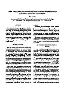
where H+ denotes the pseudoinverse of the of the hidden layer output matrix H. This solution is the best approximation for HW1 = O according to the theorem from linear algebra (see [6], [7], [9] for more details). This is equal to finding the matrix H so as to make HH+ −I = 0, where I denotes the identity matrix. However, when the rank of matrix H is low, the approximate solution can not satisfy the desired accuracy. In such a case, the task of training the network becomes equivalent to raise the rank of matrix H up to a full rank. This raising rank procedure is achieved by utilizing the nonlinearity of activation function of the networks. Once H becomes full rank, HH+ will be equal to I. To be specific, the PIL algorithm set the number of hidden neurons as N, 2 and let H = X in the initially. If ∥HH+ −I∥ is less than a pre-specified threshold, it calculates the output weights with Eq.(9). Otherwise it adds another layer and propagates the current activation value forward so as to raise the rank of matrix H layer by layer. It is worth noting that output weights can be calculated in an analytical way rather than iterative way. III. L OCALLY CONNECTED DEEP NEURAL NETWORKS A. Local connectivity Although traditional deep neural networks have been successfully used in many machine learning and pattern recognition tasks, due to the full connectivity between neurons they suffer from high model complexity which not only reduces the learning efficiency but also increases the overfitting risk. Besides, such fully connected network does not take into account the spatial structure of data, treating different dimensionality which are far apart or close together without distinction. Clearly, the fully connected network architecture is inefficient and wasteful while the huge number of parameters is associated with a greater risk of over-fitting. To address the aforementioned problems, we develop a locally connected network to substitute for the fully connected network structure. The proposed locally connected structure is

Wang et al. adopt the following pseudoinverse approximate solution to solve this optimization problem:

……

W = (HT H)−1 HT X.

W = (HT H + kI)−1 HT X, Output layer

Hidden layers

(12)

To overcome the over-fitting problem, a regularization term is added to improve the generalization performance:

……

……

……

Input layer

(11)

When the column vectors of H are linearly independent to each other, Eq.(11) can be solved as

……

……

……

……

W = H+ X.

……

……

……

……

……

……

……

……

……

……

……

……

……

……

……

Fig. 1. The locally connected network structure.

(13)

where k > 0 is a user-specified regularization parameter. In the locally connected scheme, we can train the network in a similar way by dividing the network into several sub-networks and train each one with the mentioned PIL algorithm. IV. A PPLICATION TO REAL WORLD DATA

shown in Fig. 1. In the proposed locally connected structure, it should be noted that a neuron is forced to be connected with a “segment” which is a subset of neighboring neurons in the adjacent layers. This network structure thus force the auto-encoder to learn local features which represent a spatially local input pattern. This local connectivity allows the network to first extract good features from small parts of the input data and then assemble these local representations into a unified feature vector. In addition to the local learning capability, this scheme also dramatically reduces the number of free parameters being learnt. For instance, considering an auto-encoder with 1,000 input neurons and 500 hidden neurons, the fully connected network structure would have 1,000×500+500×1,000=1,000,000 parameters (weights). Meanwhile, supposing that we divide the input data into 5 segments with equal size and the network also attempts to learn 500 dimensional features in the hidden layer from the 1,000 dimensional input data, the locally connected network would have only 200×100×5+200×100×5=200,000 parameters which are much less than the number of ones in the fully connected architecture with the same learning object. The reduce of parameters mitigates the risk of over-fitting while improves the learning efficiency.

To evaluate the efficiency and effectiveness of the proposed representation learning algorithm in astronomical spectral data, we conduct an experiment on the spectra recognition task. We divide the comparative experiment into two phases. The first one is the feature learning, in which the proposed PIL based algorithm is use for feature learning in an unsupervised way. This is followed by a classification phase. In the classification phase, we employ a softmax regression model as the classifier. For the trained network, we also visualise what hidden neurons learn and salient regions the network find given a specific spectrum as input. A. Data The data we used here are more than 50,000 stellar spectra randomly selected from LAMOST Data Release One [10]. The astronomical spectrum can be viewed as a plot of electromagnetic radiation intensity (flux) as a function of wavelength. It is a powerful tool for astrophysicists to study the properties of celestial bodies. These stellar spectra used here are labeled as F-type, G-type and K-type by the LAMOST spectral analysis

2000 1500 Flux

B. Training with PIL algorithm

2

minimize : ∥HW − X∥ . W

(10)

500 0

4000

4500

5000

5500

6000 6500 Wavelength

7000

7500

8000

8500

9000

4000

4500

5000

5500


7000

7500

8000

8500

9000

2 Normalized flux

The locally connected deep network is trained in a greedy layer-wise unsupervised way. We may regard each layer as a separated network consisting of several auto-encoders that set output to be equal to the inputs. Each auto-encoder is associated with a local segment. In Wang et al.’s previous work [4], PIL algorithm is used to training auto-encoders with imposing a additional constraint, O = X to original PIL and projecting the input data into a hidden layer with different dimensionality. Hence, the optimization object defined in Eq.(8) should be revised as

1000

1 0 −1 −2

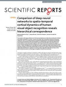
Fig. 2. Top to bottom: A random sample of raw spectra; the sample after preprocessing.

pipeline. These spectra cover the range 3,650-9,000 angstrom with a resolution R>1,800. Before employing our algorithm in spectra recognition, we need to perform a series of preprocessing for the raw spectral data. For a given input data set i d D = {xi , oi }N i=1 , where a vector x = (x1 , x2 ,...,xd ) ∈ R represents a spectrum. Here, d = 3, 601 and xi represents the flux at a certain wavelength. We down sample the spectrum to form a 721 dimensional vector. This preprocessing can reduce the complexity of the network with little to no effect on predictive performance and thus improves the learning efficiency. It should be noted that the fluxes in different wavelengths of the spectra vary greatly, that is, the range of values in different dimensionality of raw data varies widely. Therefore, it is necessary to perform the whitening normalization first. The comparison between the raw spectrum and the preprocessed one is shown in Fig. 2. B. Settings In this experiment, we compare our algorithm with other techniques employed in astronomy in terms of the feature learning time and accuracy. The accuracy is calculated as acc =

N 1 ∑ 1{f (xi ) = y i }, N i=1

TABLE I C OMPARISON BETWEEN PIL BASED AND OTHER

ALGORITHMS ON

SPECTRA

Algorithm PILDNN PILDNN* RBM PCA LLE

Feature Learning Time (seconds) 226.9495 1,103.4251 1,481.0040 1.9056 2,539.9331

Accuracy 0.8190 0.8232 0.7572 0.7464 0.7749

learning technique, the elapsed training time is more than 20 hours while our algorithm only needs several minutes. The reason why pseudoinverse based approach can improve the computational efficiency comparing to conventional deep learning algorithms is that it pre-trains the deep model analytically while the conventional algorithms require iterative optimization. Furthermore, unlike conventional deep learning models, we do not adopt a time-consuming global fine-tuning and simply employ a perceptor as the classifier. Besides, The local connectivity scheme also speeds up the learning procedure, which can be observed in the comparison between the PILDNN and PILDNN*.

(14)

where f (xi ) and y i denote the predicted label and true label, respectively. 1{·} takes on a value of 1 if its argument is true, and 0 otherwise. Bu et al. [11] apply RBM to spectral processing. Although RBM is always used as a building block to train deep models, Bu et al. use a single RBM rather than stack RBMs into a deep model. In additional, we also compare our proposed method with principal component analysis (PCA) and Locally Linear Embedding (LLE), both of which are widely used in spectra unsupervised feature extraction in astronomy [12], [13], [14], [15]. In this experiment, we training the neural network in two different way including our proposed training algorithm and the naive implementation with full connectivity. In the local connectivity scheme, the input spectra are split into 4 segments. To ensure the fairness of evaluation, both networks have the same architecture with layers of size 721-400-800-1,200-2,000-3, which means a network has 721 inputs corresponding to the dimensionality of re-binned spectrum, 4 hidden layers with 400, 800, 1,200 and 2,000 neurons, respectively and 3 outputs representing the 3 classes. C. Results TABLE I demonstrates the results of comparison on the spectral data. PILDNN and PILDNN* denote the PIL based deep neural networks with and without local connectivity, respectively. Comparison of the results obtained shows that our method has obvious advantages over conventional methods in accuracy. The reason lies in the limitation of shallow models, which means deep architectures might be able to represent more complicated functions while simpler and shallower architectures fail to represent. Although the deep model has better capacity, if we train it with the conventional deep

D. Visualizing and analysis The proposed deep neural networks with the efficient learning algorithm have demonstrated impressive performance on the real world spectral data. However this deep model still remains a black box since the activations in intermediate layers are very difficult to understand and there is also no clear understanding of how the model operates, why it achieves such good performance, or what it exactly learns from a standpoint of machine learning. Without clear understanding of the features in intermediate layers and what exactly the networks learn from the data, we could only develop or improve a model by trial-and-error. In this subsection, we aim at addressing two problems. The first one is to find good qualitative interpretations of what a neuron learns in hidden layers. The second one is to explore ways of visualizing the salient regions in the input space specific to a given spectrum. As to the first problem, we reproduce the input patterns which maximize the activation of a given hidden neuron with imposing a norm constraint to avoiding trivial solution. The reasoning behind this idea is that the input patterns maximizing the activation of a given hidden neuron illustrate what the neuron is looking for in such input space. Inspired by D. Erhan et al.’s work [16], we can consider the idea of maximizing the activation of a given neuron as an optimization problem. To be specific, Let Θ denote our neural network parameter set which includes connection weights and the bias. let hij denotes the i-th neuron in the j-th layer of the network. hij (Θ, x) can be viewed as a function mapping an input sample x to the activation of the given neuron. For a trained network, Θ is fixed, we can formulate the optimization problem as x∗ = arg max hij (Θ, x),

(15)

Flux

1 0.5

Flux

0 1 0.5

Flux

0 1 0.5

Flux

0 1 0.5

Flux

0 1 0.5

Flux

0 1 0.5 0

4000

4200

4400 Wavelength

4600

4800

4800

5000

5200


5800

6000 6000

6200

6400


7000

7200

7200 7400 7600 7800 8000 8200 8400 8600 8800 9000 Wavelength

Fig. 3. Visualization of patterns learnt by hidden neurons given a random selected spectrum as input. The top row shows the 4 input spectrum segments. For rows 2 to 6 we show the patterns which maximize the activation of the top 5 active neurons for each segment separately. The wavelengths are given in angstroms.

1

Flux

1

1

1

1

0.8

0.8

0.8

0.8

0.8

0.6

0.6

0.6

0.6

0.6

0.4

0.4

0.4

0.4

0.4

0.2

0.2

0.2

0.2

0.2

0

0

0

0

0

Flux

Flux

1

1

1

0.8

0.8

0.8

0.8

0.8

0.6

0.6

0.6

0.6

0.6

0.4

0.4

0.4

0.4

0.4

0.2

0.2

0.2

0.2

0.2

0

0

0

0

0

1

1

1

1

1

0.8

0.8

0.8

0.8

0.8

0.6

0.6

0.6

0.6

0.6

0.4

0.4

0.4

0.4

0.4

0.2

0.2

0.2

0.2

0.2

0

0

0

0

4000

5000


8000

9000

4000

5000


8000

9000

4000

5000


8000

9000

0 4000

5000


8000

9000

Fig. 4. Visualization of the importance of input patterns for the predicted results in three random selected spectra with different labels. We cover up different portions of the input spectra with a sliding window to see how the final classifier output changes. Rows 1 to 3 show the three sampled spectra separately. The size of the sliding window is specified as 1, 64, 128, 256 respectively in the columns 1 to 4. The wavelengths are given in angstroms.

where x∗ is the input pattern maximizing the activation of the given neuron and can be viewed as what this neuron has learnt. To be specific, an input sample is presented to the trained network and propagated throughout the first j layers. Then we can select top n most active neurons in the j-th layer and map values of these neurons back to the input layer by solving the aforementioned optimization problem. Since the most commonly used activation functions, e.g., the sigmoidal function and the hyperbolic function, are both continuous and have continuous first derivatives, the optimization problem can be solved with a gradient-based method. Fig. 3 shows what

neurons learn in the hidden layers of our model when the training has completed. For a given input spectrum consisting of 4 segments, we select top 5 most active neurons in an arbitrary hidden layer corresponding to each segments and map each activation separately back to the input space. The obtained patterns in the input space reveal the learning results of the selected hidden neurons. It can be observed that learnt patterns are similar to the input spectrum, which prove that the model is capable of learning the features of both continuum and strong lines. As to the second problem, we are inspired by Zeiler and

Fergus’s work [17] and evaluate the importance of different portions (sub-patterns) in the input sample by visualising the changes in the output space. In other words, each portion is assigned a contribution value to the final prediction. To this end, we occlude different parts of the input sample with a sliding window, and visualising the change in the output neuron. By doing this, we can get a function which maps the position of the sliding window to the saliency of the occluded portion. If occluding a certain portion causes a significant change in the final prediction, we can conclude that the network is more attentive to the certain patterns lying in the occluded portion. It should be noted that a portion may be occluded several times by the sliding window, hence we calculate the overall saliency by taking an average of them. The visualization is presented in Fig. 4 where the color reflects the relative importance of the individual pixels. A light-colored region therefore means that these portions of the input spectrum are important evidence for the predicted class, and support this decision. A dark-colored region means that these portions are unrelated to the prediction or even against the predicted class. For instance, we can see that almost the entire spectra are painted in dark color in the first column of Fig. 4. It implies that the trained network dose not “think” that any portions in the sliding windows provides important evidence for the final prediction. In fact, the window size is only 1 thus any single pixel in it actually provides little information for the final prediction. With the sliding window size increasing, it is interesting to observe how the network assess the importance of different input sub-patterns. With a proper window size, it can be observed that the trained network is more attentive to the portions near to the peak of blackbody radiation intensity. It is well known that the peak wavelength is associated with the temperatures of hot radiant objects, which is the criterion of stellar spectral classification. The importance of different input sub-patterns learnt by the network in turn reflects the capacity of the network to extract information with higher distinguishability. V. C ONCLUSIONS In this paper, we designed a deep neural network with locally connected structure and of which is trained with an efficient pseudoinverse learning algorithm. Compared with other baseline algorithms, our algorithm has obvious advantage in learning speed. In addition, with a locally connected network structure, even if the data dimension is large, the computation of pseudoinverse is also not the hard work because “divide and conquer” strategy is adopted. The capability and generality of our method is verified in an astronomical spectrum recognition application, the results demonstrate that our method is superior in the comprehensive performance. We also visualize and analyze the features learnt in hidden layers and what exactly the network learn from the data. In the future work, we also plan to apply our representation learning algorithm to other astronomical tasks such as special objects retrieval, defect spectra repairing in addition to the spectra recognition discussed in this paper.

ACKNOWLEDGMENT This work is fully supported by the grants from the National Natural Science Foundation of China (61375045), Beijing Natural Science Foundation (4142030) and the Joint Research Fund in Astronomy (U1531242) under cooperative agreement between the National Natural Science Foundation of China (NSFC) and Chinese Academy of Sciences (CAS). Dr. Ping Guo and Xin Xin are the authors to whom all the correspondence should be addressed. R EFERENCES [1] Y. Bengio, A. Courville, and P. Vincent, “Representation Learning: A Review and New Perspectives,” IEEE Transactions on Pattern Analysis and Machine Intelligence, vol. 35, no. 8, pp. 1798–1828, 2013. [2] G. Hinton and R. Salakhutdinov, “Reducing the Dimensionality of Data with Neural Networks,” Science, vol. 313, no. 5786, pp. 504–507, 2006. [3] Y. Bengio, “Learning deep architectures for AI,” Foundations and trends in Machine Learning, vol. 2, no. 1, pp. 1–127, 2009. [4] K. Wang, P. Guo, Q. Yin, A. Luo and X. Xin, “A Pseudoinverse Incremental Algorithm for Fast Training Deep Neural Networks with Application to Spectra Pattern Recognition,” in 2014 International Joint Conference on Neural Networks (IJCNN), Vancouver, Canada, Jul. 2016, in press. [5] X. Cui et al., “The Large Sky Area Multi-Object Fiber Spectroscopic Telescope (LAMOST),” Research in Astronomy and Astrophysics, vol. 12, no. 9, pp. 1197–1242, 2012. [6] P. Guo and M. Lyu, “Pseudoinverse Learning Algorithm for Feedforward Neural Networks,” in Advances in Neural Networks and Applications, (N. E. Mastorakis, Ed.), Puerto De La Cruz, Tenerife, Canary Islands, Spain, Feb. 2001, pp. 321–326. [7] P. Guo and M. Lyu, “A pseudoinverse learning algorithm for feedforward neural networks with stacked generalization applications to software reliability growth data,” Neurocomputing, vol. 56, pp. 101–121, 2004. [8] X. Glorot, A. Bordes, and Y. Bengio, “Deep sparse rectifier neural networks”, in the Fourteenth International Conference on Artificial Intelligence and Statistics (AISTATS 2011), Fort Lauderdale, USA, Apr. 2011, pp. 315–323. [9] T. Boullion and P. Odell, “Generalized Inverse Matrices”, John Wiley and Sons, Inc., New York, 1971. [10] A. Luo et al., “The first data release (DR1) of the LAMOST regular survey,”. Research in Astronomy and Astrophysics, vol. 15, no. 8, pp. 1095–1124, 2015. [11] Y. Bu, G. Zhao, A. Luo, J. Pan, and Y. Chen, “Restricted Boltzmann machine: a non-linear substitute for PCA in spectral processing”, Astronomy and Astrophysics, vol. 576, A96, 2015. [12] C. Whitney, “Principal components analysis of spectral data. IMethodology for spectral classification”, Astronomy and Astrophysics Supplement Series, vol. 51, pp. 443–461, 1983. [13] A. Connolly and A. Szalay, “A robust classification of galaxy spectra: Dealing with noisy and incomplete data,” The Astronomical Journal, vol. 117, no. 5, pp. 2052, 1999. [14] J. VanderPlas and A. Connolly, “Reducing the dimensionality of data: Locally linear embedding of sloan galaxy spectra”, The Astronomical Journal, vol. 138, no. 5, pp. 1365, 2009. [15] S. Daniel, A. Connolly, J. Schneider, J. VanderPlas, and L. Xiong, “Classification of stellar spectra with local linear embedding”, The Astronomical Journal, vol .142, no. 6, pp. 203, 2011. [16] D. Erhan, Y. Bengio, A. Courville, and P. Vincent, “Visualizing higherlayer features of a deep network,” University of Montreal, Tech. Rep, 2009. [17] M. Zeiler and R. Fergus, “Visualizing and understanding convolutional networks,” Computer Vision-ECCV 2014-13th European Conference, Zurich, Switzerland, Sep. 2014.