Dec 5, 2016 - recent examples in cyber security and autonomous vehicles. Despite the ... investigate this issue shared across previous research work and to propose a ...... examples taken from the DREBIN Android malware dataset.
Oct 4, 2016 - R. Giryes is with the School of Electrical Engineering, Faculty of Engineering, ... the Jacobian matrix of encoder for regularization of auto-encoders [27], ... constraints are usually enforced by training networks with weight decay ...
May 23, 2017 - Jure Sokolic, Student Member, IEEE, Raja Giryes, Member, IEEE, ... of Raja Giryes was supported in part by GIF, the German-Israeli Foundation ...
performance by deep learning relative to other machine learning approaches ... To verify the idea we study the use of auxiliary pose information to improve the ...
~Afl+ i;u!f' + 7~:: + FX~? :quaternion output of. (In particular. = 1 represent the bias inputs ,F;' n= 1,. . No is the input signal and Ff = n= 1,. ., Nu is the output). 4 0 ...
[12] P. Ginzberg and A. T. Walden, âTesting for quaternion propriety,â IEEE. Trans. Signal Process., vol.59, pp. 3025-3034, 2011. [13] J. VÃa, D. RamÃrez and L.
Mar 3, 2017 - experiments conducted on the designed benchmark reflect a successful congestion ...... Theano: A Python framework for fast com- putation of ...
Pooling Layer: The pooling layers apply a (usually) non-linear transform (Note that the ... which takes us one step closer to make an implementable network in ...
By analysing patterns of captured data from a network, IDS help to ... With the increasing value of big data, deep networks is an important element to capture in ...
Aug 21, 2017 - We evaluate the positioning accuracy of state-of-the-art CNNs with channel ... Index TermsâDeep Learning, Convolutional Neural Networks,.
Mar 14, 2017 - gained great attention of the research community [1, 2]. There is an ..... [17] A. Graves, A. rahman Mohamed, and G. Hinton, âSpeech recogni-.
Jun 16, 2017 - . Proceedings of the 34th ...... Yao, Yuan, Rosasco, Lorenzo, and Caponnetto, Andrea. On early stopping in ...
Jun 22, 2015 - We achieve a Dice Similarity Coefficient of 83.6±6.3% in training ..... K. Mori, and D. Rueckert (2013). Auto- mated abdominal multi-organ ...
for the class of cartoon functions introduced by Donoho, 2001. I. INTRODUCTION. Feature extractors based on so-called deep convolutional neural networks ...
Jan 27, 2015 - be extended to the more AI oriented domain of move pre- diction in Go. ... encoding schemes and network d
Jun 7, 2017 - Subset400: randomly selected 400 items from the test set. 4Music by a female vocalist is more often tagged as female vocalists than.
Jun 16, 2017 - Proceedings of the 34th International Conference on Machine. Learning, Sydney, Australia ..... We call x a critical sample if there exists a point x ..... was financially supported by the Samsung Advanced In- stitute of Technology ...
Apr 8, 2017 - Index TermsâDeep learning, convolutional neural network, dynamic ..... Output k-space samples ... xu. DS. C1. C2 ... Cndâ1. Crec xcnn xcnn. F.
Feb 17, 2018 - power of the network while keeping it simple by choosing best features. Based on such principles, we propose a simple architec- ture called ...
point arrays perform the multiply and add in the analog domain in contrast to the CMOS based digital approaches. Therefore, it is not clear yet whether the ...
Jul 2, 2016 - At the same time, it becomes .... is the use of l1 regularization, wherein we penalize the sum ...... gpu math compiler in python,â in Proc.
1Athinoula A. Martinos Center for Biomedical Imaging, Department of Radiology,. Massachusetts General ...... The Cancer Imaging Archive. (2016). Available at:.
Mar 30, 2018 - after the penultimate max-pooling layer and r = 4 for the last two newly ..... GT: ground truth saliency maps; DCL+: DCL with CRF refinement.
Feb 20, 2018 - we set a maximum compressed size ratio and had the ...... Ehsan Variani, Chanwoo Kim, Olivier Siohan, Mit
cjg7182@louisiana.edu. Anthony S. ... is a normalization technique called batch normalization [1] ... method can be seen in Highway Networks [2] and Residual.
arXiv:1712.04604v2 [cs.NE] 30 Jan 2018
Deep Quaternion Networks Chase J. Gaudet
Anthony S. Maida
School of Computing & Informatics University of Lousiana at Lafayette Lafayette, USA [email protected]
School of Computing & Informatics University of Lousiana at Lafayette Lafayette, USA [email protected]
Abstract—The field of deep learning has seen significant advancement in recent years. However, much of the existing work has been focused on real-valued numbers. Recent work has shown that a deep learning system using the complex numbers can be deeper for a fixed parameter budget compared to its real-valued counterpart. In this work, we explore the benefits of generalizing one step further into the hyper-complex numbers, quaternions specifically, and provide the architecture components needed to build deep quaternion networks. We go over quaternion convolutions, present a quaternion weight initialization scheme, and present algorithms for quaternion batch-normalization. These pieces are tested in a classification model by end-to-end training on the CIFAR-10 and CIFAR-100 data sets and a segmentation model by end-to-end training on the KITTI Road Segmentation data set. The quaternion networks show improved convergence compared to real-valued and complex-valued networks, especially on the segmentation task. Index Terms—quaternion, complex, neural networks, deep learning
I. I NTRODUCTION There have been many advances in deep neural network architectures in the past few years. One such improvement is a normalization technique called batch normalization [1] that standardizes the activations of layers inside a network using minibatch statistics. It has been shown to regularize the network as well as provide faster and more stable training. Another improvement comes from architectures that add so called shortcut paths to the network. These shortcut paths connect later layers to earlier layers typically, which allows for the stronger gradients to propagate to the earlier layers. This method can be seen in Highway Networks [2] and Residual Networks [3]. Other work has been done to find new activation functions with more desirable properties. One example is the exponential linear unit (ELU) [4], which attempts to keep activations standardized. All of the above methods are combating the vanishing gradient problem [5] that plagues deep architectures. With solutions to this problem appearing it is only natural to move to a system that will allow one to construct deeper architectures with as low a parameter cost as possible. Other work in this area has explored the use of complex and hyper-complex numbers, which are a generalization of the complex, such as quaternions. Using complex numbers in recurrent neural networks (RNNs) has been shown to increase learning speed and provide a more noise robust memory retrieval mechanism [6]–[8]. The first formulation of
complex batch normalization and complex weight initialization is presented by [9] where they achieve some state of the art results on the MusicNet data set. Hyper-complex numbers are less explored in neural networks, but have seen use in manual image and signal processing techniques [10]–[12]. Examples of using quaternion values in networks is mostly limited to architectures that take in quaternion inputs or predict quaternion outputs, but do not have quaternion weight values [13], [14]. There are some more recent examples of building models that use quaternions represented as real-values. In [15] they used a quaternion multi-layer perceptron (QMLP) for document understanding and [16] uses a similar approach in processing multi-dimensional signals. Building on [9] our contribution in this paper is to formulate and implement quaternion convolution, batch normalization, and weight initialization 1 . There arises some difficulty over complex batch normalization that we had to overcome as their is no analytic form for our inverse square root matrix. II. M OTIVATION AND R ELATED W ORK The ability of quaternions to effectively represent spatial transformations and analyze multi-dimensional signals makes them promising for applications in artificial intelligence. One common use of quaternions is for representing rotation into a more compact form. PoseNet [14] used a quaternion as the target output in their model where the goal was to recover the 6−DOF camera pose from a single RGB image. The ability to encode rotations may make a quaternion network more robust to rotational variance. Quaternion representation has also been used in signal processing. The amount of information in the phase of an image has been shown to be sufficient to recover the majority of information encoded in its magnitude by Oppenheim and Lin [17]. The phase also encodes information such as shapes, edges, and orientations. Quaternions can be represented as a 2 x 2 matrix of complex numbers, which gives them a group of phases potentially holding more information compared to a single phase. Bulow and Sommer [12] used the higher complexity representation of quaternions by extending Gabor’s complex signal to a quaternion one which was then used for texture segmentation. Another use of quaternion filters is shown in [11] where 1 Source
code located at https://github.com/gaudetcj/DeepQuaternionNetworks
they introduce a new class of filter based on convolution with hyper-complex masks, and present three color edge detecting filters. These filters rely on a three-space rotation about the grey line of RGB space and when applied to a color image produce an almost greyscale image with color edges where the original image had a sharp change of color. More quaternion filter use is shown in [18] where they show that it is effective in the context of segmenting color images into regions of similar color texture. They state the advantage of using quaternion arithmetic is that a color can be represented and analyzed as a single entity, which we will see holds for quaternion convolution in a convolutional neural network architecture as well in Section III-C. A quaternionic extension of a feed forward neural network, for processing multi-dimensional signals, is shown in [16]. They expect that quaternion neurons operate on multidimensional signals as single entities, rather than real-valued neurons that deal with each element of signals independently. A convolutional neural network (CNN) should be able to learn a powerful set of quaternion filters for more impressive tasks. Another large motivation is discussed in [9], which is that complex numbers are more efficient and provide more robust memory mechanisms compared to the reals [10]–[12]. They continue that residual networks have a similar architecture to associative memories since the residual shortcut paths compute their residual and then sum it into the memory provided by the identity connection. Again, given that quaternions can be represented as a complex group, they may provide an even more efficient and robust memory mechanisms. III. Q UATERNION N ETWORK C OMPONENTS This section will include the work done to obtain a working deep quaternion network. Some of the longer derivations are given in the Appendix. A. Quaternion Representation
This representation of quaternions is not unique, but we will stick to the above in this paper. It is also possible to represent H as M (2, C) where M (2, C) is a 2 x 2 complex matrix. With our real-valued representation a quaternion real-valued 2D convolution layer can be expressed as follows. Say that the layer has N feature maps such that N is divisible by 4. We let the first N/4 feature maps represent the real components, the second N/4 represent the i imaginary components, the third N/4 represent the j imaginary components, and the last N/4 represent the k imaginary components. B. Quaternion Differentiability
In 1833 Hamilton proposed complex numbers C be defined as the set R2 of ordered pairs (a, b) of real numbers. He then began working to see if triplets (a, b, c) could extend multiplication of complex numbers. In 1843 he discovered a way to multiply in four dimensions instead of three, but the multiplication lost commutativity. This construction is now known as quaternions. Quaternions are composed of four components, one real part, and three imaginary parts. Typically denoted as H = {a + bi + cj + dk : a, b, c, d ∈ R}
Since we will be performing quaternion arithmetic using reals it is useful to embed H into a real-valued representation. There exists an injective homomorphism from H to the matrix ring M (4, R) where M (4, R) is a 4x4 real matrix. The 4 x 4 matrix can be written as a −b −c −d 1 0 0 0 b a −d c = a 0 1 0 0 c d 0 0 1 0 a −b d −c b a 0 0 0 1 0 −1 0 0 1 0 0 0 + b 0 0 0 −1 0 0 1 0 0 0 −1 0 0 0 0 1 + c 1 0 0 0 0 −1 0 0 0 0 0 −1 0 0 −1 0 . (4) + d 0 1 0 0 1 0 0 0
(1)
In order for the network to perform backpropagation the cost function and activation functions used must be differentiable with respect to the real, i, j, and k components of each quaternion parameter of the network. As the complex chain rule is shown in [9], we provide the quaternion chain rule which is given in the Appendix section VII-A. C. Quaternion Convolution
where a is the real part, (i, j, k) denotes the three imaginary axis, and (b, c, d) denotes the three imaginary components. Quaternions are governed by the following arithmetic:
Convolution in the quaternion domain is done by convolving a quaternion filter matrix W = A+iB+jC+kD by a quaternion vector h = w + ix + jy + kz. Performing the convolution by using the distributive property and grouping terms one gets
i2 = j 2 = k 2 = ijk = −1
(2)
W ∗ h = (A ∗ w − B ∗ x − C ∗ y − D ∗ z)+
which, by enforcing distributivity, leads to the noncommutative multiplication rules
i(A ∗ x + B ∗ w + C ∗ z − D ∗ y)+ j(A ∗ y − B ∗ z + C ∗ w + D ∗ x)+
ij = k, jk = i, ki = j, ji = −k, kj = −i, ik = −j (3)
k(A ∗ z + B ∗ y − C ∗ x + D ∗ w).
(5)
Using a matrix to represent the components of the convolution we have:
R(W ∗ h) A I (W ∗ h) B J (W ∗ h) = C K (W ∗ h) D
−B A D −C
−C −D w x −D C ∗ A −B y B A z
(6)
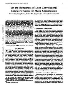
An example is shown in Fig. 1 where one can see how quaternion convolution forces a linear depthwise mixture of the channels. This is similar to a mixture of standard convolution and depthwise separable convolution from [19]. This reuse of filters on every layer and combination may help extract texture information across channels as seen in [18].
sition of V−1 where V is the covariance matrix given by: Vrr Vri Vrj Vrk Vir Vii Vij Vik V = Vjr Vji Vjj Vjk Vkr Vki Vkj Vkk Cov(R{x}, R{x}) Cov(I {x}, R{x}) = Cov(J {x}, R{x}) Cov(K {x}, R{x}) Cov(R{x}, I {x}) Cov(I {x}, I {x}) Cov(J {x}, I {x}) Cov(K {x}, I {x}) Cov(R{x}, J {x}) Cov(I {x}, J {x}) Cov(J {x}, J {x}) Cov(K {x}, J {x}) Cov(R{x}, K {x}) Cov(I {x}, K {x}) Cov(J {x}, K {x}) Cov(K {x}, K {x})
D. Quaternion Batch-Normalization
Batch-normalization [1] is used by the vast majority of all deep networks to stabilize and speed up training. It works by keeping the activations of the network at zero mean and unit variance. The original formulation of batch-normalization only works for real-values. Applying batch normalization to complex or hyper-complex numbers is more difficult, one can not simply translate and scale them such that their mean is 0 and their variance is 1. This would not give equal variance in the multiple components of a complex or hyper-complex number. To overcome this for complex numbers a whitening approach is used [9], which scales the data by the square root of their variances along each of the two principle components. We use the same approach, but must whiten 4D vectors. However, an issue arises in that there is no nice way to calculate the inverse square root of a 4 x 4 matrix. It turns out that the square root is not necessary and we can instead use the Cholesky decomposition on our covariance matrix. The details of why this works for whitening given in the Appendix section VII-B. Now our whitening is accomplished by multiplying the 0-centered data (x − E[x]) by W:
x ˜ = W(x − E[x])
(7)
where Cov(·) is the covariance and R{x}, I {x}, J {x}, and K {x} are the real, i, j, and k components of x respectively. Real-valued batch normalization also uses two learned parameters, β and γ. Our shift parameter β must shift a quaternion value so it is a quaternion value itself with real, i, j, and k as learnable components. The scaling parameter γ is a symmetric matrix of size matching V given by: Vrr Vri Vrj Vrk Vri Vii Vij Vik γ= (9) Vrj Vij Vjj Vjk Vrk Vik Vjk Vkk Because of its symmetry it has only ten learnable parameters. The variance of the components of input √ ˜x are variance 1 so the diagonal of γ is initialized to 1/ 16 in order to obtain a modulus of 1 for the variance of the normalized value. The off diagonal terms of γ and all components of β are initialized to 0. The quaternion batch normalization is defined as: BN(˜x) = γ˜x + β
(10)
E. Quaternion Weight Initialization The proper initialization of weights is vital to convergence of deep networks. In this work we derive our quaternion weight initialization using the same procedure as Glorot and Bengio [20] and He et al. [21]. To begin we find the variance of a quaternion weight: W = |W |e(cosφ1 i+cosφ2 j+cosφ3 k)θ = R{W } + I {W } + J {W } + K {W }.
where W is one of the matrices from the Cholesky decompo-
(8)
(11)
where |W | is the magnitude, θ and φ are angle arguments, and cos2 φ1 + cos2 φ2 + cos2 φ3 = 1 [22].
Fig. 1. An illustration of quaternion convolution.
Variance is defined as Var(W ) = E[|W |2 ] − (E[W ])2 ,
(12)
but since W is symmetric around 0 the term (E[W ])2 is 0. We do not have a way to calculate Var(W ) = E[|W |2 ] so we make use of the magnitude of quaternion normal values |W |, which follows an independent normal distribution with four degrees of freedom (DOFs). We can then calculate the expected value of |W |2 to find our variance Z ∞ E[|W |2 ] = x2 f (x) dx = 4σ 2 (13) ∞
where f (x) is the four DOF distribution given in the Appendix. And since Var(W ) = E[|W |2 ], we now have the variance of W expressed in terms of a single parameter σ: Var(W ) = 4σ 2 .
(14)
To follow the Glorot and Bengio [20] initialization we have Var(W ) = 2/(nin +nout ), where nin and nout are the number of input and output units respectivly. p Setting this equal to (14) and solving for σ gives σ = 1/ 2(nin + nout ). To follow He et al. [21] initialization that is specialized for rectified linear units (ReLUs) [23], then we have Var(W ) = 2/nin , which √ again setting equal to (14) and solving for σ gives σ = 1/ 2nin . As shown in (11) the weight has components |W |, θ, and φ. We can initialize the magnitude |W | using our four DOF distribution defined with the appropriate σ based on which initialization scheme we are following. The angle components are initialized using the uniform distribution between −π and π where we ensure the constraint on φ. IV. E XPERIMENTAL R ESULTS Our experiments covered image classification using both the CIFAR-10 and CIFAR-100 benchmarks and image segmentation using the KITTI Road Estimation benchmark. A. Classification We use the same architecture as the large model in [9], which is a 110 layer Residual model similar to the one in [3]. There is one difference between the real-valued network and the ones used for both the complex and hyper-complex valued networks. Because the datasets are all real-valued the network must learn the imaginary or quaternion components. We use the same technique as [9] where there is an additional block immediately after the input which will learn the hypercomplex components BN → ReLU → Conv → BN → ReLU → Conv. Since all datasets that we work with are real-valued, we present a way to learn their imaginary components to let the rest of the network operate in the complex plane. We learn the initial imaginary component of our input by performing the operations present within a single real-valued residual block
This means that to maintain the same approximate parameter count the number of convolution kernels for the complex network was increased. We however did not increase the number of convolution kernels for the quaternion trials so any increase in model performance comes from the quaternion filters and at a lower hardware budget. The architecture consists of 3 stages of repeating residual blocks where at the end of each stage the images are downsized by strided convolutions. Each stage also doubles the previous stage’s number of convolution kernels. The last layers are a global average pooling layer followed by a single fully connected layer with a softmax function used to classify the input as either one of the 10 classes in CIFAR-10 or one of the 100 classes in CIFAR-100. We also followed their training procedure of using the backpropagation algorithm with Stochastic Gradient Descent with Nesterov momentum [24] set at 0.9. The norm of the gradients are clipped to 1 and a custom learning rate scheduler is used. The learning scheduler is the same used in [9] for a direct comparison in performance. The learning rate is initially set to 0.01 for the first 10 epochs and then set it to 0.1 from epoch 10-100 and then cut by a factor of 10 at epochs 120 and 150. Table I presents our results along side the real and complex valued networks. Our quaternion model outperforms the real and complex networks on both datasets on a smaller parameter budget. Architecture [3] Real [9] Complex Quaternion
CIFAR-10 CIFAR-100 6.37 5.60 27.09 5.44 26.01 TABLE I C LASSIFICATION ERROR ON CIFAR-10 AND CIFAR-100. N OTE THAT [3] IS A 110 LAYER RESIDUAL NETWORK , [9] IS 118 LAYER COMPLEX NETWORK WITH THE SAME DESIGN AS THE PRIOR EXCEPT WITH ADDITIONAL INITIAL LAYERS TO EXTRACT COMPLEX MAPPINGS .
B. Segmentation For this experiment we used the same model as the above, but cut the number of residual blocks out of the model for memory reasons given that the KITTI data is large color images. The 110 layer model has 10, 9, and 9 residual blocks in the 3 stages talked about above, while this model has 2, 1, and 1 and does not perform any strided convolutions. This gives a total of 38 layers. The last layer is a 1 × 1 convolution with a sigmoid output so we are getting a heatmap prediction the same size as the input. The training procedure is also as above, but the learning rate is scheduled differently. Here we begin at 0.01 for the first 10 epochs and then set it to 0.1 from epoch 10-50 and then cut by a factor of 10 at 100 and 150. Table II presents our results along side the real and complex valued networks where we used Intersection over Union (IOU) for performance measure. Quaternion outperformed the other two by a larger margin compared to the classification tasks.
Architecture KITTI Real 0.747 Complex 0.769 Quaternion 0.827 TABLE II IOU ON KITTI ROAD E STIMATION BENCHMARK .
V. C ONCLUSIONS We have extended upon work looking into complex valued networks by exploring quaternion values. We presented the building blocks required to build and train deep quaternion networks and used them to test residual architectures on two common image classification benchmarks. We show that they have competitive performance by beating both the real and complex valued networks with less parameters. Future work will be needed to test quaternion networks for more segmentation datasets and for audio processing tasks. VI. ACKNOWLEDGMENT
[15] T. Parcollet, M. Morchid, P.-M. Bousquet, R. Dufour, G. Linar`es, and R. De Mori, “Quaternion neural networks for spoken language understanding,” in Spoken Language Technology Workshop (SLT), 2016 IEEE, pp. 362–368, IEEE, 2016. [16] T. Minemoto, T. Isokawa, H. Nishimura, and N. Matsui, “Feed forward neural network with random quaternionic neurons,” Signal Processing, vol. 136, pp. 59–68, 2017. [17] A. V. Oppenheim and J. S. Lim, “The importance of phase in signals,” Proceedings of the IEEE, vol. 69, no. 5, pp. 529–541, 1981. [18] L. Shi and B. Funt, “Quaternion color texture segmentation,” Computer Vision and image understanding, vol. 107, no. 1, pp. 88–96, 2007. [19] F. Chollet, “Xception: Deep learning with depthwise separable convolutions,” arXiv preprint arXiv:1610.02357, 2016. [20] X. Glorot and Y. Bengio, “Understanding the difficulty of training deep feedforward neural networks,” in Proceedings of the Thirteenth International Conference on Artificial Intelligence and Statistics, pp. 249–256, 2010. [21] K. He, X. Zhang, S. Ren, and J. Sun, “Delving deep into rectifiers: Surpassing human-level performance on imagenet classification,” in Proceedings of the IEEE international conference on computer vision, pp. 1026–1034, 2015. [22] R. Piziak and D. Turner, “The polar form of a quaternion,” 2002.
We would like to thank James Dent of the University of Louisiana at Lafayette Physics Department for helpful discussions. We also thank Fugro for research time on this project.
[23] V. Nair and G. E. Hinton, “Rectified linear units improve restricted boltzmann machines,” in Proceedings of the 27th international conference on machine learning (ICML-10), pp. 807–814, 2010.
R EFERENCES
[25] A. Kessy, A. Lewin, and K. Strimmer, “Optimal whitening and decorrelation,” The American Statistician, no. just-accepted, 2017.
[1] S. Ioffe and C. Szegedy, “Batch normalization: Accelerating deep network training by reducing internal covariate shift,” in International Conference on Machine Learning, pp. 448–456, 2015. [2] R. K. Srivastava, K. Greff, and J. Schmidhuber, “Training very deep networks,” in Advances in neural information processing systems, pp. 2377– 2385, 2015. [3] K. He, X. Zhang, S. Ren, and J. Sun, “Deep residual learning for image recognition,” in Proceedings of the IEEE conference on computer vision and pattern recognition, pp. 770–778, 2016. [4] D.-A. Clevert, T. Unterthiner, and S. Hochreiter, “Fast and accurate deep network learning by exponential linear units (elus),” arXiv preprint arXiv:1511.07289, 2015. [5] S. Hochreiter, “Untersuchungen zu dynamischen neuronalen netzen,” Diploma, Technische Universit¨at M¨unchen, vol. 91, 1991. [6] M. Arjovsky, A. Shah, and Y. Bengio, “Unitary evolution recurrent neural networks,” in International Conference on Machine Learning, pp. 1120–1128, 2016. [7] I. Danihelka, G. Wayne, B. Uria, N. Kalchbrenner, and A. Graves, “Associative long short-term memory,” arXiv preprint arXiv:1602.03032, 2016. [8] S. Wisdom, T. Powers, J. Hershey, J. Le Roux, and L. Atlas, “Fullcapacity unitary recurrent neural networks,” in Advances in Neural Information Processing Systems, pp. 4880–4888, 2016. [9] C. Trabelsi, O. Bilaniuk, D. Serdyuk, S. Subramanian, J. F. Santos, S. Mehri, N. Rostamzadeh, Y. Bengio, and C. J. Pal, “Deep complex networks,” arXiv preprint arXiv:1705.09792, 2017. [10] T. B¨ulow, Hypercomplex spectral signal representations for the processing and analysis of images. Universit¨at Kiel. Institut f¨ur Informatik und Praktische Mathematik, 1999. [11] S. J. Sangwine and T. A. Ell, “Colour image filters based on hypercomplex convolution,” IEE Proceedings-Vision, Image and Signal Processing, vol. 147, no. 2, pp. 89–93, 2000. [12] T. Bulow and G. Sommer, “Hypercomplex signals-a novel extension of the analytic signal to the multidimensional case,” IEEE Transactions on signal processing, vol. 49, no. 11, pp. 2844–2852, 2001. [13] A. Rishiyur, “Neural networks with complex and quaternion inputs,” arXiv preprint cs/0607090, 2006. [14] A. Kendall, M. Grimes, and R. Cipolla, “Posenet: A convolutional network for real-time 6-dof camera relocalization,” in Proceedings of the IEEE international conference on computer vision, pp. 2938–2946, 2015.
[24] Y. Nesterov, “A method of solving a convex programming problem with convergence rate o (1/k2),”
VII. A PPENDIX
A. The Generalized Quaternion Chain Rule for a Real-Valued Function
We start by specifying the Jacobian. Let L be a real valued loss function and q be a quaternion variable such that q = a + i b + j c + k d where a, b, c, d ∈ R then,
E[ZZT ] = I E[W(X − µ)(W(X − µ))T ] = I E[W(X − µ)(X − µ)T WT ] = I WΣWT = I WΣWT W = W WT W = Σ−1
(18)
From (18) it is clear that the Cholesky decomposition provides a suitable (but not unique) method of finding W. C. Cholesky Decomposition Cholesky decomposition is an efficient way to implement LU decomposition for symmetric matrices, which allows us to find the square root. Consider AX = b, A = [aij ]n×n , and aij = aji , then the Cholesky decomposition of A is given by A = LL0 where l11 0 . . . 0 .. l21 l22 . . . . (19) L= . . . . . . . . 0 . ln1 ln2 ... lnn Let lki be the k th row and ith column entry of L, then k