Deep Syntactic Processing by Combining Shallow Methods - CiteSeerX

Proceedings of the 41st Annual Meeting of the Association for Computational Linguistics, July 2003, pp. 431-438.

Deep Syntactic Processing by Combining Shallow Methods P´eter Dienes and Amit Dubey Department of Computational Linguistics Saarland University PO Box 15 11 50 66041 Saarbr¨ucken, Germany {dienes,adubey}@coli.uni-sb.de

Abstract We present a novel approach for finding discontinuities that outperforms previously published results on this task. Rather than using a deeper grammar formalism, our system combines a simple unlexicalized PCFG parser with a shallow pre-processor. This pre-processor, which we call a trace tagger, does surprisingly well on detecting where discontinuities can occur without using phase structure information.

1 Introduction In this paper, we explore a novel approach for finding long-distance dependencies. In particular, we detect such dependencies, or discontinuities, in a two-step process: (i) a conceptually simple shallow tagger looks for sites of discontinuties as a preprocessing step, before parsing; (ii) the parser then finds the dependent constituent (antecedent). Clearly, information about long-distance relationships is vital for semantic interpretation. However, such constructions prove to be difficult for stochastic parsers (Collins et al., 1999) and they either avoid tackling the problem (Charniak, 2000; Bod, 2003) or only deal with a subset of the problematic cases (Collins, 1997). Johnson (2002) proposes an algorithm that is able to find long-distance dependencies, as a postprocessing step, after parsing. Although this algorithm fares well, it faces the problem that stochastic parsers not designed to capture non-local dependencies may get confused when parsing a sentence with

discontinuities. However, the approach presented here is not susceptible to this shortcoming as it finds discontinuties before parsing. Overall, we present three primary contributions. First, we extend the mechanism of adding gap variables for nodes dominating a site of discontinuity (Collins, 1997). This approach allows even a context-free parser to reliably recover antecedents, given prior information about where discontinuities occur. Second, we introduce a simple yet novel finite-state tagger that gives exactly this information to the parser. Finally, we show that the combination of the finite-state mechanism, the parser, and our new method for antecedent recovery can competently analyze discontinuities. The overall organization of the paper is as follows. First, Section 2 sketches the material we use for the experiments in the paper. In Section 3, we propose a modification to a simple PCFG parser that allows it to reliably find antecedents if it knows the sites of long-distance dependencies. Then, in Section 4, we develop a finite-state system that gives the parser exactly that information with fairly high accuracy. We combine the models in Section 5 to recover antecedents. Section 6 discusses related work.

2 Annotation of empty elements Different linguistic theories offer various treatments of non-local head–dependent relations (referred to by several other terms such as extraction, discontinuity, movement or long-distance dependencies). The underlying idea, however, is the same: extraction sites are marked in the syntactic structure and this mark is connected (co-indexed) to the control-

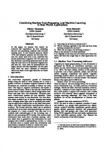
Type NP – NP WH – NP PRO – NP COMP – SBAR UNIT WH – S WH – ADVP CLAUSE COMP – WHNP ALL

Freq. 987 438 426 338 332 228 120 118 98 3310

Example

SBAR

Sam was seen * the woman who you saw * T *

S     

NP

* to sleep is nice

who

Sam said 0 Sasha snores

VP     

NP

$ 25 * U *

you

Sam had to go, Sasha said * T * Sam told us how he did it * T *

saw

Sam had to go, Sasha said 0 the woman 0 we saw * T *

Table 1: Most frequent types of EE s in Section 0.

ling constituent. The experiments reported here rely on a training corpus annotated with non-local dependencies as well as phrase-structure information. We used the Wall Street Journal (WSJ) part of the Penn Treebank (Marcus et al., 1993), where extraction is represented by co-indexing an empty terminal element (henceforth EE ) to its antecedent. Without committing ourselves to any syntactic theory, we adopt this representation. Following the annotation guidelines (Bies et al., 1995), we distinguish seven basic types of EE s: controlled NP -traces (NP ), PRO s (PRO ), traces of A -movement (mostly wh-movement: WH), empty complementizers (COMP ), empty units (UNIT ), and traces representing pseudo-attachments (shared constituents, discontinuous dependencies, etc.: PSEUDO ) and ellipsis (ELLIPSIS ). These labels, however, do not identify the EE s uniquely: for instance, the label WH may represent an extracted NP object as well as an adverb moved out of the verb phrase. In order to facilitate antecedent recovery and to disambiguate the EE s, we also annotate them with their parent nodes. Furthermore, to ease straightforward comparison with previous work (Johnson, 2002), a new label CLAUSE is introduced for COMP - SBAR whenever it is followed by a moved clause WH – S . Table 1 summarizes the most frequent types occurring in the development data, Section 0 of the WSJ corpus, and gives an example for each, following Johnson (2002). For the parsing and antecedent recovery experiments, in the case of WH-traces (WH –


) and

V

NP     

* WH - NP *

Figure 1: Threading gap+WH-NP. controlled NP -traces (NP – NP ), we follow the standard technique of marking nodes dominating the empty element up to but not including the parent of the antecedent as defective (missing an argument) with a gap feature (Gazdar et al., 1985; Collins, 1997).1 Furthermore, to make antecedent co-indexation possible with many types of EE s, we generalize Collins’ approach by enriching the annotation of non-terminals with the type of the EE in question (eg. WH – NP ) by using different gap+ features (gap+WH-NP; cf. Figure 1). The original nonterminals augmented with gap+ features serve as new non-terminal labels. In the experiments, Sections 2–21 were used to train the models, Section 0 served as a development set for testing and improving models, whereas we present the results on the standard test set, Section 23.

3 Parsing with empty elements The present section explores whether an unlexicalized PCFG parser can handle non-local dependencies: first, is it able to detect EE s and, second, can it find their antecedents? The answer to the first question turns out to be negative: due to efficiency reasons and the inappropriateness of the model, detecting all types of EE s is not feasible within the parser. Antecedents, however, can be reliably recovered provided a parser has perfect knowledge about EE s occurring in the input. This shows that the main bottleneck is detecting the EE s and not finding their antecedents. In the following section, therefore, we explore how we can provide the parser with information about EE sites in the current sentence without 1 This

technique fails for 82 sentences of the treebank where the antecedent does not c-command the corresponding EE.

relying on phrase structure information. 3.1

Method

There are three modifications required to allow a parser to detect EE s and resolve antecedents. First, it should be able to insert empty nodes. Second, it must thread the gap+ variables to the parent node of the antecedent. Knowing this node is not enough, though. Since the Penn Treebank grammar is not binary-branching, the final task is to decide which child of this node is the actual antecedent. The first two modifications are not difficult conceptually. A bottom-up parser can be easily modified to insert empty elements (c.f. Dienes and Dubey (2003)). Likewise, the changes required to include gap+ categories are not complicated: we simply add the gap+ features to the nonterminal category labels. The final and perhaps most important concern with developing a gap-threading parser is to ensure it is possible to choose the correct child as the antecedent of an EE . To achieve this task, we employ the algorithm presented in Figure 2. At any node in the tree where the children, all together, have more gap+ features activated than the parent, the algorithm deduces that a gap+ must have an antecedent. It then picks a child as the antecedent and recursively removes the gap+ feature corresponding to its EE from the non-terminal labels. The algorithm has a shortcoming, though: it cannot reliably handle cases when the antecedent does not c-command its EE . This mostly happens with PSEUDO s (pseudo-attachments), where the algorithm gives up and (wrongly) assumes they have no antecedent. Given the perfect trees of the development set, the antecedent recovery algorithm finds the correct antecedent with 95% accuracy, rising to 98% if PSEUDO s are excluded. Most of the remaining mistakes are caused either by annotation errors, or by binding NP -traces (NP – NP ) to adjunct NP s, as opposed to subject NPs. The parsing experiments are carried out with an unlexicalized PCFG augmented with the antecedent recovery algorithm. We use an unlexicalized model to emphasize the point that even a simple model detects long distance dependencies successfully. The parser uses beam thresholding (Goodman, 1998) to

for a tree T , iterate over nodes bottom-up for a node with rule P C0


Cn N  multiset of E E s in P M  multiset of E E s in C0


Cn foreach E E of type e in M  N pick a j such that e allows C j as an antecedent  pick a k such that k  j and Ck dominates an E E of type e if no such j or k exist, return no antecedent else bind the E E dominated by Ck to the antecedent C j

Figure 2: The antecedent recovery algorithm. ensure efficient parsing. PCFG probabilities are calculated in the standard way (Charniak, 1993). In order to keep the number of independently tunable parameters low, no smoothing is used. The parser is tested under two different conditions. First, to assess the upper bound an EE detecting unlexicalized PCFG can achieve, the input of the parser contains the empty elements as separate words (PERFECT ). Second, we let the parser introduce the EE s itself (INSERT ). 3.2

Evaluation

We evaluate on all sentences in the test section of the treebank. As our interest lies in trace detection and antecedent recovery, we adopt the evaluation measures introduced by Johnson (2002). An EE is correctly detected if our model gives it the correct label as well as the correct position (the words before and after it). When evaluating antecedent recovery, the EE s are regarded as four-tuples, consisting of the type of the EE , its location, the type of its antecedent and the location(s) (beginning and end) of the antecedent. An antecedent is correctly recovered if all four values match the gold standard. The precision, recall, and the combined F-score is presented for each experiment. Missed parses are ignored for evaluation purposes. 3.3

Results

The main results for the two conditions are summarized in Table 2. In the INSERT case, the parser detects empty elements with precision 64.7%, recall 40.3% and F-Score 49.7%. It recovers antecedents

Condition Empty element detection (F-score) Antecedent recovery (F-score) Parsing time (sec/sent) Missed parses

PERFECT

INSERT

–

49 7%

91 4%

43 0%

25 1 6%

21 44 3%

  wi  X; wi
1  X;   wi 1 X X is a prefix of wi ,  X  4 X is a suffix of wi , X 4 wi contains a number wi contains uppercase character wi contains hyphen li
1  X posi  X; posi
1  X; posi  1 posi
1 posi  XY posi
2 posi
1 posi  XY Z posi posi  1  XY posi posi  1 posi  2  XY Z

Table 2: EE detection, antecedent recovery, parsing times, and missed parses for the parser



X

Table 3: Local features at position i  1. with overall precision 55.7%, recall 35.0% and Fscore 43.0%. With a beam width of 1000, about half of the parses were missed, and successful parses take, on average, 21 seconds per sentence and enumerate 1.7 million edges. Increasing the beam size to 40000 decreases the number of missed parses marginally, while parsing time increases to nearly two minutes per sentence, with 2.9 million edges enumerated. In the PERFECT case, when the sites of the empty elements are known before parsing, only about 1.6% of the parses are missed and average parsing time goes down to 2 5 seconds per sentence. More importantly, the overall precision and recall of antecedent recovery is 91.4%. 3.4

Discussion

The result of the experiment where the parser is to detect long-distance dependencies is negative. The parser misses too many parses, regardless of the beam size. This cannot be due to the lack of smoothing: the model with perfect information about the EE -sites does not run into the same problem. Hence, the edges necessary to construct the required parse are available but, in the INSERT case, the beam search loses them due to unwanted local edges having a higher probability. Doing an exhaustive search might help in principle, but it is infeasible in practice. Clearly, the problem is with the parsing model: an unlexicalized PCFG parser is not able to detect where EE s can occur, hence necessary edges get low probability and are, thus, filtered out. The most interesting result, though, is the difference in speed and in antecedent recovery accuracy between the parser that inserts traces, and the parser which uses perfect information from the treebank about the sites of EE s. Thus, the question

naturally arises: could EE s be detected before parsing? The benefit would be two-fold: EE s might be found more reliably with a different module, and the parser would be fast and accurate in recovering antecedents. In the next section we show that it is indeed possible to detect EE s without explicit knowledge of phrase structure, using a simple finite-state tagger.

4 Detecting empty elements This section shows that EE s can be detected fairly reliably before parsing, i.e. without using phrase structure information. Specifically, we develop a finite-state tagger which inserts EE s at the appropriate sites. It is, however, unable to find the antecedents for the EE s; therefore, in the next section, we combine the tagger with the PCFG parser to recover the antecedents. 4.1

Method

Detecting empty elements can be regarded as a simple tagging task: we tag words according to the existence and type of empty elements preceding them. For example, the word Sasha in the sentence Sam said COMP – SBAR Sasha snores. will get the tag EE = COMP – SBAR , whereas the word Sam is tagged with EE =* expressing the lack of an EE immediately preceding it. If a word is preceded by more than one EE , such as to in the following example, it is tagged with the concatenation of the two EE s, i.e., EE = COMP – WHNP PRO – NP . It would have been too late COMP – WHNP PRO – NP to think about on Friday.

Target NP – NP NP – NP PRO - NP




WH – ADVP UNIT

Explanation passive to-infinitive

[,:]  ( V ,)

gerund lookahead for that

N

COMP – SBAR WH – NP

Matching regexp BE RB * VBN RB * to RB * VB

! IN

 

RB * VBG  !that * ( MD  V )

WP WDT COMP – WHNP



! WH – NP *

lookback for pending WHNPs

V

WRB ! WH – ADVP* V ! WH – ADVP* $ CD*

[.,:]

lookback for pending WHADVP before a verb $ sign before numbers

Table 4: Non-local binary feature templates; the EE -site is indicated by Although this approach is closely related to POStagging, there are certain differences which make this task more difficult. Despite the smaller tagset, the data exhibits extreme sparseness: even though more than 50% of the sentences in the Penn Treebank contain some EE s, the actual number of EE s is very small. In Section 0 of the WSJ corpus, out of the 46451 tokens only 3056 are preceded by one or more EE s, that is, approximately 93.5% of the words are tagged with the EE =* tag. The other main difference is the apparently nonlocal nature of the problem, which motivates our choice of a Maximum Entropy (ME) model for the tagging task (Berger et al., 1996). ME allows the flexible combination of different sources of information, i.e., local and long-distance cues characterizing possible sites for EE s. In the ME framework, linguistic cues are represented by (binary-valued) features ( fi ), the relative importance (weight, λ i ) of which is determined by an iterative training algorithm. The weighted linear combination of the features amount to the log-probability of the label (l) given the context (c): p  l c 

1 exp  ∑i λi fi  l c 

Z  c

(1)

where Z  c is a context-dependent normalizing factor to ensure that p  l c be a proper probability distribution. We determine weights for the features with a modified version of the Generative Iterative Scaling algorithm (Curran and Clark, 2003). Templates for local features are similar to the ones employed by Ratnaparkhi (1996) for POS-tagging (Table 3), though as our input already includes POStags, we can make use of part-of-speech information as well. Long-distance features are simple hand-

written regular expressions matching possible sites for EE s (Table 4). Features and labels occurring less than 10 times in the training corpus are ignored. Since our main aim is to show that finding empty elements can be done fairly accurately without using a parser, the input to the tagger is a POS-tagged corpus, containing no syntactic information. The best label-sequence is approximated by a bigram Viterbi-search algorithm, augmented with variable width beam-search. 4.2

Results

The results of the EE -detection experiment are summarized in Table 5. The overall unlabeled F-score is 85 3%, whereas the labeled F-score is 79 1%, which amounts to 97 9% word-level tagging accuracy. For straightforward comparison with Johnson’s results, we must conflate the categories PRO – NP and NP – NP . If the trace detector does not need to differentiate between these two categories, a distinction that is indeed important for semantic analysis, the overall labeled F-score increases to 83 0%, which outperforms Johnson’s approach by 4%. 4.3

Discussion

The success of the trace detector is surprising, especially if compared to Johnson’s algorithm which uses the output of a parser. The tagger can reliably detect extraction sites without explicit knowledge of the phrase structure. This shows that, in English, extraction can only occur at well-defined sites, where local cues are generally strong. Indeed, the strength of the model lies in detecting such sites (empty units, UNIT ; NP traces, NP – NP ) or where clear-cut long-distance cues exist (WH – S , COMP – SBAR ). The accuracy of detecting uncon-

EE

LABELED UNLABELED NP – NP WH – NP PRO – NP COMP – SBAR UNIT WH – S WH – ADVP CLAUSE COMP – WHNP

Prec. Here 86.5% 93.3% 87.8% 92.5% 68.7% 93.8% 99.1% 94.4% 81.6% 80.4% 67.2%

Rec. Here 72.9% 78.6% 79.6% 75.6% 70.4% 78.6% 92.5% 91.3% 46.8% 68.3% 38.3%

F-score Here Johnson 79.1% – 85.3% – 83.5% – 83.2% 81.0% 69.5% – 85.5% 88.0% 95.7% 92.0% 92.8% 87.0% 59.5% 56.0% 73.8% 70.0% 48.8% 47.0%

Table 5: EE -detection results on Section 23 and comparison with Johnson (2002) (where applicable).

trolled PRO s (PRO – NP ) is rather low, since it is a difficult task to tell them apart from NP traces: they are confused in 10 15% of the cases. Furthermore, the model is unable to capture for. . . to+INF constructions if the noun-phrase is long. The precision of detecting long-distance NP extraction (WH – NP ) is also high, but recall is lower: in general, the model finds extracted NP s with overt complementizers. Detection of null WHcomplementizers (COMP – WHNP ), however, is fairly inaccurate (48 8% F-score), since finding it and the corresponding WH – NP requires information about the transitivity of the verb. The performance of the model is also low (59 5%) in detecting movement sites for extracted WH-adverbs (WH – ADVP ) despite the presence of unambiguous cues (where, how, etc. starting the subordinate clause). The difficulty of the task lies in finding the correct verb-phrase as well as the end of the verb-phrase the constituent is extracted from without knowing phrase boundaries. One important limitation of the shallow approach described here is its inability to find the antecedents of the EE s, which clearly requires knowledge of phrase structure. In the next section, we show that the shallow trace detector and the unlexicalized PCFG parser can be coupled to efficiently and successfully tackle antecedent recovery.

Condition Antecedent recovery (F-score) Parsing time (sec/sent) Missed parses

NOINSERT

INSERT

72 6%

69 3%

27 2 4%

25 5 3%

Table 6: Antecedent recovery, parsing times, and missed parses for the combined model

5 Combining the models In Section 3, we found that parsing with EE s is only feasible if the parser knows the location of EE s before parsing. In Section 4, we presented a finite-state tagger which detects these sites before parsing takes place. In this section, we validate the two-step approach, by applying the parser to the output of the trace tagger, and comparing the antecedent recovery accuracy to Johnson (2002). 5.1

Method

Theoretically, the ‘best’ way to combine the trace tagger and the parsing algorithm would be to build a unified probabilistic model. However, the nature of the models are quite different: the finite-state model is conditional, taking the words as given. The parsing model, on the other hand, is generative, treating the words as an unlikely event. There is a reasonable basis for building the probability models in different ways. Most of the tags emitted by the EE tagger are just EE =*, which would defeat generative models by making the ‘hidden’ state uninformative. Conditional parsing algorithms do exist, but they are difficult to train using large corpora (Johnson, 2001). However, we show that it is quite effective if the parser simply treats the output of the tagger as a certainty. Given this combination method, there still are two interesting variations: we may use only the EE s proposed by the tagger (henceforth the NOINSERT model), or we may allow the parser to insert even more EE s (henceforth the INSERT model). In both cases, EE s outputted by the tagger are treated as separate words, as in the PERFECT model of Section 3. 5.2

Results

The NOINSERT model did better at antecedent detection (see Table 6) than the INSERT model. The

Type OVERALL NP – NP WH – NP PRO – NP COMP – SBAR UNIT WH – S WH – ADVP CLAUSE COMP – WHNP

Prec. Here 80.5% 71.2% 91.6% 68.7% 93.8% 99.1% 86.7% 67.1% 80.4% 67.2%

Rec. Here 66.0% 62.8% 71.9% 70.4% 78.6% 92.5% 83.9% 31.3% 68.3% 38.8%

F-score Here Johnson 72.6% 68.0% 66.8% 60.0% 80.6% 80.0% 69.5% 50.0% 85.5% 88.0% 95.7% 92.0% 84.8% 87.0% 42.7% 56.0% 73.8% 70.0% 48.8% 47.0%

Table 7: Antecedent recovery results for the combined NOINSERT model and comparison with Johnson (2002).

NOINSERT model was also faster, taking on average 2.7 seconds per sentence and enumerating about 160,000 edges whereas the INSERT model took 25 seconds on average and enumerated 2 million edges. The coverage of the NOINSERT model was higher than that of the INSERT model, missing 2.4% of all parses versus 5.3% for the INSERT model.

Comparing our results to Johnson (2002), we find that the NOINSERT model outperforms that of Johnson by 4.6% (see Table 7). The strength of this system lies in its ability to tell unbound PRO s and bound NP – NP traces apart. 5.3

Discussion

Combining the finite-state tagger with the parser seems to be invaluable for EE detection and antecedent recovery. Paradoxically, taking the combination to the extreme by allowing both the parser and the tagger to insert EE s performed worse. While the INSERT model here did have wider coverage than the parser in Section 3, it seems the real benefit of using the combined approach is to let the simple model reduce the search space of the more complicated parsing model. This search space reduction works because the shallow finitestate method takes information about adjacent words into account, whereas the context-free parser does not, since a phrase boundary might separate them.

6 Related Work Excluding Johnson (2002)’s pattern-matching algorithm, most recent work on finding head– dependencies with statistical parser has used statistical versions of deep grammar formalisms, such as CCG (Clark et al., 2002) or LFG (Riezler et al., 2002). While these systems should, in theory, be able to handle discontinuities accurately, there has not yet been a study on how these systems handle such phenomena overall. The tagger presented here is not the first one proposed to recover syntactic information deeper than part-of-speech tags. For example, supertagging (Joshi and Bangalore, 1994) also aims to do more meaningful syntactic pre-processing. Unlike supertagging, our approach only focuses on detecting EE s. The idea of threading EE s to their antecedents in a stochastic parser was proposed by Collins (1997), following the GPSG tradition (Gazdar et al., 1985). However, we extend it to capture all types of EE s.

7 Conclusions This paper has three main contributions. First, we show that gap+ features, encoding necessary information for antecedent recovery, do not incur any substantial computational overhead. Second, the paper demonstrates that a shallow finite-state model can be successful in detecting sites for discontinuity, a task which is generally understood to require deep syntactic and lexical-semantic knowledge. The results show that, at least in English, local clues for discontinuity are abundant. This opens up the possibility of employing shallow finite-state methods in novel situations to exploit non-apparent local information. Our final contribution, but the one we wish to emphasize the most, is that the combination of two orthogonal shallow models can be successful at solving tasks which are well beyond their individual power. The accent here is on orthogonality – the two models take different sources of information into account. The tagger makes good use of adjacency at the word level, but is unable to handle deeper recursive structures. A context-free grammar is better at finding vertical phrase structure, but cannot exploit linear information when words are separated

by phrase boundaries. As a consequence, the finitestate method helps the parser by efficiently and reliably pruning the search-space of the more complicated PCFG model. The benefits are immediate: the parser is not only faster but more accurate in recovering antecedents. The real power of the finite-state model is that it uses information the parser cannot.

Acknowledgements The authors would like to thank Jason Baldridge, Matthew Crocker, Geert-Jan Kruijff, Miles Osborne and the anonymous reviewers for many helpful comments.

References Adam L. Berger, Stephen A. Della Pietra, and Vincent J. Della Pietra. 1996. A maximum entropy approach to natural language processing. Computational Linguistics, 22(1):39–71. Ann Bies, Mark Ferguson, Karen Katz, and Robert MacIntyre, 1995. Bracketting Guidelines for Treebank II style Penn Treebank Project. Linguistic Data Consortium. Rens Bod. 2003. An efficient implementation of a new dop model. In Proceedings of the 11th Conference of the European Chapter of the Association for Computational Linguistics, Budapest. Eugene Charniak. 1993. Statistical Language Learning. MIT Press, Cambridge, MA. Eugene Charniak. 2000. A maximum-entropy-inspired parser. In Proceedings of the 1st Conference of North American Chapter of the Association for Computational Linguistics, Seattle, WA. Stephen Clark, Julia Hockenmaier, and Mark Steedman. 2002. Building deep dependency structures with a wide-coverage CCG parser. In Proceedings of the 40th Annual Meeting of the Association for Computational Linguistics, Philadelphia. Michael Collins, Jan Hajiˇc, Lance Ramshaw, and Christoph Tillmann. 1999. A statistical parser for Czech. In Proceedings of the 37th Annual Meeting of the Association for Computational Linguistics, University of Maryland, College Park. Michael Collins. 1997. Three generative, lexicalised models for statistical parsing. In Proceedings of the 35th Annual Meeting of the Association for Computational Linguistics and the 8th Conference of the European Chapter of the Association for Computational Linguistics, Madrid.

James R. Curran and Stephen Clark. 2003. Investigating GIS and smoothing for maximum entropy taggers. In Proceedings of the 11th Annual Meeting of the European Chapter of the Association for Computational Linguistics, Budapest, Hungary. P´eter Dienes and Amit Dubey. 2003. Antecedent recovery: Experiments with a trace tagger. In Proceedings of the Conference on Empirical Methods in Natural Language Processing, Sapporo, Japan. Gerald Gazdar, Ewan Klein, Geoffrey Pullum, and Ivan Sag. 1985. Generalized Phase Structure Grammar. Basil Blackwell, Oxford, England. Joshua Goodman. 1998. Parsing inside-out. Ph.D. thesis, Harvard University. Mark Johnson. 2001. Joint and conditional estimation of tagging and parsing models. In Proceedings of the 39th Annual Meeting of the Association for Computational Linguistics and the 10th Conference of the European Chapter of the Association for Computational Linguistics, Toulouse. Mark Johnson. 2002. A simple pattern-matching algorithm for recovering empty nodes and their antecedents. In Proceedings of the 40th Annual Meeting of the Association for Computational Linguistics, Philadelphia. Aravind K. Joshi and Srinivas Bangalore. 1994. Complexity of descriptives–supertag disambiguation or almost parsing. In Proceedings of the 1994 International Conference on Computational Linguistics (COLING-94), Kyoto, Japan. Mitchell P. Marcus, Beatrice Santorini, and Mary Ann Marcinkiewicz. 1993. Building a large annotated corpus of English: The Penn Treebank. Computational Linguistics, 19(2):313–330. Adwait Ratnaparkhi. 1996. A Maximum Entropy Partof-Speech tagger. In Proceedings of the Empirical Methods in Natural Language Processing Conference. University of Pennsylvania. Stefan Riezler, Tracy H. King, Ronald M. Kaplan, Richard Crouch, John T. Maxwell, and Mark Johnson. 2002. Parsing the Wall Street Journal using a Lexical-Functional Grammar and discriminative estimation techniques. In Proceedings of the 40th Annual Meeting of the Association for Computational Linguistics, Philadelphia.