Default Risk Codependence in the Global Financial System: Was the Bear Stearns Bailout Justified?
Jorge A. Chan-Lau*
International Monetary Fund and The Fletcher School of Law and Diplomacy, Tufts University Email:
[email protected] Preliminary Please do not circulate
December 2008
_________ * The views expressed in this paper do not reflect those of IMF nor IMF policy. The author is solely responsible for any errors or omissions.
2
Default Risk Codependence in the Global Financial System: Was the Bear Stearns Bailout Justified?
Abstract The current subprime crisis has encouraged renewed efforts to understand systemic risk. The assessment of systemic risk requires measuring default risk codependence, or in other words, how the default risk of a specific institution affects the conditional default risk of another institution. This paper proposes a methodology for assessing default risk codependence among financial institutions based on quantile regression after accounting for the impact of fundamental and technical factors. Results are reported for a sample of 25 financial institutions in Europe, Japan, and the United States. Consistent with the earlier contagion literature, the results indicate that risk codependence is stronger during distress periods. The results also cast some light on the controversy surrounding the bailout of Bear Stearns and AIG, and the bankruptcy of Lehman Brothers and suggest that there is room for improving information disclosure and transparency in regards to policy decisions.
Keywords: default risk, systemic risk, contagion, financial institutions, quantile regression. JEL Classification: G21, G14, F37, C20
3 1.
Why Risk Codependence Matters
The increased globalization of financial markets, the deepening of financial integration, and the rapid pace of financial innovation have created a global financial system that transcends national boundaries. While the system has brought substantial benefits such as increased capital flows, lower borrowing costs, and better price discovery and risk diversification, the system has also strengthened and created news channels for the transmission of negative shocks across borders and across markets. The worldwide financial crisis that started in 2007 is a stark reminder of the risks posed by a more integrated and globalized financial system. The 2007–8 crisis has encouraged renewed efforts in four interconnected areas: the definition and measurement of systemic risk, the development of early warning indicators of financial crises, the enhancement of supervisory and regulatory frameworks, and the strengthening of current crisis management and bank resolution frameworks. Work in these four areas is currently under way in central banks and multilateral financial institutions as policy makers attempt to find an effective and prompt solution to the problems posed by the crisis and seek to avoid future crises. This paper contributes to work in the first area, the measurement of systemic risk, by proposing a methodology for assessing default risk codependence among financial institutions. Risk codependence is defined as the default risk of one institution conditional on the default risk of another institution after correcting for the effect of common observable fundamental and technical factors. Default risk codependence, therefore, is a manifestation of contagion that can be implied from observable security prices. Given observed default risk measures, it is possible to construct risk codependence measures using quantile regression. Why does risk codependence matters? Risk codependence is closely linked to contagion and financial crises spillovers. In this context the measures of risk codependence derived in this paper are associated with unobservable factors likely related to the interconnectedness among financial institutions. The interconnectedness arises from direct linkages, such as counterparty risk from interbank claims, or indirect linkages such as exposure to common risk factor such as reliance on wholesale markets for funding and feedback effects from market volatility due to the adoption of similar risk management and accounting practices. When markets are efficient, these linkages are priced in by market participants and lead to comovements among institutions’ security prices and risk measures as market participants. 1
1
Common risk measures for financial institutions include distance-to-default, credit default swaps spreads, and the VaR of their trading portfolios. All these measures depend on market data and are considered forwardlooking since current prices should reflect market expectations of earnings and discount rates.
4 The results obtained from analyzing credit default swap spreads for a sample of 25 financial institutions in Europe, Japan, and the United States suggest that risk codependence is stronger during distress periods, a finding consistent with the earlier empirical literature on contagion. More interestingly, the results also cast some light on the controversy surrounding the bailout of Bear Stearns and AIG, and the bankruptcy of Lehman Brothers. Contagion effects, as implied from credit default swap spreadsdo not appear to justify the policy decision to bailout AIG and Bear Stearns instead of Lehman Brothers. In the latter case, the apparent contradiction between what markets imply and the policy decision suggests that credit derivatives markets exhibit, at best, semi-strong efficiency and do not incorporate private information. 2 It also suggests that there is room for improving the communication of private information relevant to policy decisions. The remainder of this paper is structured as follows. Section 2 explains why quantile regression is appropriate for measuring risk codependence among financial institutions. Section 3 describes in detail the specification of the econometric model and defines two measures of conditional risk codependence. Section 4 describes the data used to estimate the risk codependence measures and section 5 presents and analyzes the results. Section 6 concludes. 2.
Measuring Risk Codependence using Quantile Regressions
For risk management, regulatory, and surveillance purposes it is important to design and implement measures of risk codependence that account for large negative shocks. Accordingly, extreme-value theory measures appear suitable for capturing the risk codependence of institutions subject to large negative shocks. 3 One common problem associated to extreme value measures, though, is that a significant amount of information from the whole data sample is lost as the analysis uses only the tail realizations of the series. This problem is more acute the shorter the length of the data sample is. As an alternative to extreme value theory, this paper introduces two conditional codependence measures that use all the information available in the sample. The measure is constructed using quantile regression, a simple approach that helps examining how risk codependence changes conditional on the level of risk of an individual institution. 4
2
Fama (1970).
3
See among others Hartman, Straetmans and De Vries (2001); Chan-Lau, Mathieson and Yao (2004); and references therein.
4
We extend the analysis of Adrian and Brunnermeier (2008). For a detailed exposition of quantile regression techniques, see Koenker (2005), and for an intuitive exposition, Koenker and Hallock (2001).
5 Quantile regression is a technique that expands on standard least squares estimation and provides an extensive analysis of the relationship among random variables. Quantile regression extends the notions of ordering, sorting and ranking the data by ascending (or descending) order of univariate statistical analysis to regression models. As a result, it is possible to estimate the functional relationship among variables at different quantiles. In other words, in addition to computing the conditional mean function, as done through ordinary least squares, quantile regression also computes the full family of conditional quantile functions. The use of conditional quantile functions in addition to the conditional mean function is important in the presence of regime switches since functional relationships may differ from one regime to the other. The existence of a multi-regime approach is usually assumed formally or intuitively when analyzing the impact of a financial crisis and the appropriate policy responses. In the empirical literature on contagion and financial crises, at least two different regimes are usually identified: a tranquil regime and a volatile regime. The volatile regime is usually characterized by rapidly falling security prices and a substantial increase of the risk of institutions. In the context of quantile regression, if risk measures or security prices are sorted by quantiles, the tranquil regime and volatile regimes are associated with the lower and higher conditional quantile functions respectively. In the context of the current crisis, moreover, there is a special emphasis on designing a regulatory framework where policy measures are contingent on whether the economy is in a pre-crisis, crisis, or post-crisis regime. 5
Before describing the methodology in detail, we review briefly some other ways to measure systemic risk in the financial sector that complement the approach in this paper. Equity price comovements could be used as a proxy for risk codependence in the financial system since they exhibit a high degree of commonality. 6 Furthermore, equity return data has also been used to estimate the probability of the simultaneous defaults of a group of banks. 7 Similarly, the availability of prices for credit default swaps, which are insurance-like contracts, and estimates of asset return correlation derived from equity returns can be used to construct a default probability-based measure of systemic. 8
5
See Financial Stability Forum (2008) and the special issued of the Journal of Financial Stability edited by Goodhart (2008).
6
Hawkesby, Marsh, and Stevens (2007).
7
Lehar (2005) and Allenspach and Monnin (2006).
8
Huang, Zhou, and Zhu (2008).
6 3.
Model Specification and Risk Codependence Measures
As explained in Koenker and Hallock (2001), given N observations, the estimation of a quantile regression relies on the minimization of the sum of residuals. The residuals are weighted asymmetrically according to: (1)
N
min ∑ ρτ ( y i − ξ ( xi , β )) , β
i
where y is the dependent variable, ξ ( xi , β ) is a linear function of the parameters, and (2)
ρτ (u ) = u (τ − 1(u < 0) ) ,
is the residual weight function for the quantile τ . The minimization can be solved using standard linear programming techniques and the covariance matrices are usually estimated using bootstrap techniques which are valid even if the residuals and explanatory variables are not independent (Koenker, 2005). When analyzing risk codependence, the relevant issue is to assess how the risk of institution i, denoted by Risk i , is affected by the risk of institution j, denoted by Risk j , after correcting for the effect of K aggregate risk factors, Rk . The aggregate risk factors account for the impact of fundamental factors such as the stage of the business cycle and technical factors such as investor sentiment. The minimization problem of interest, therefore, is given by: (3)
N
K
i
k
min ∑ ρτ ( Risk i − ∑ β k ,τ Rk − β j ,τ Risk j )) . β
The equation above is solved for different quantiles τ in order to examine how the risk codependence between any two firms varies at different levels of risk. Indeed, the risk codependence is implicitly captured by the set of parameters β j ,τ so we will refer to this coefficient as the risk codependence coefficient. The behavior of β j ,τ as a function of τ illustrates how the risk of institution j affects institution i. An upward sloping pattern suggests that the riskier institution j is, the greater the impact is on the risk of institution i. Therefore, we can interpret the coefficient β j ,τ as a risk codependence measure. Furthermore, since the quantile regressions include aggregate observable risk factors, the coefficient β j ,τ can be interpreted as a proxy for the “frailty” effect, or an unobserved latent risk factor. Empirical studies using data on U.S. corporations
7 suggest that the frailty effect is an important explanatory factor of correlated default in the sector. 9 In addition to examining the behavior of β j ,τ as a function of τ , it is also possible to quantify the risk codependence between institutions i and j in terms of the conditional codependence function for a specific quantile, as first suggested by Adrian and Brunnermeier (2008). The conditional risk codependence measure, or CRC measure, is defined as: CoRisk ij (τ ) = {Risk i (τ ) | Risk j (τ ), R K },
(4)
where Riski (τ ) is the level of risk of firm i for quantile τ . An alternative way to express the conditional risk measure is in terms of percent increase in the unconditional risk of firm i:
⎛ {Risk i (τ ) | Risk j (τ ), RK } ⎞ CoRisk ij (τ )(in percent ) = 100 × ⎜⎜ − 1⎟⎟ Risk i (τ ) ⎠ ⎝
(5)
The next section describes the data used to estimate equation (3) and its associated conditional risk codependence coefficient, β j ,τ , and construct the CRC measure. 4.
Data
The quantile regressions were estimated using daily market data for the period July 1, 2003 – September 30, 2008. One advantage of using market data is that market data is available at high frequencies and on a timely fashion. Another advantage is that, provided market efficiency holds, market data is forward looking in general and captures market expectations on changes in the risk and performance of financial institutions. Yields, spreads, and equity returns were obtained from Primark Datastream; credit default swap mid-price quotes were obtained from Blooomberg and Primark Datatream. The U.S. institutions included in this study are AIG, Bank of America, Bear Stearns, Citigroup, Goldman Sachs, JP Morgan, Lehman Brothers, Merrill Lynch, Morgan Stanley, Wachovia, and Wells Fargo; the European institutions are Fortis, Banque Nationale Paribas, Societe Generale, Deusche Bank, Commerzbank, BBVA, Santander, Credit Suisse, UBS, Barclays, and HSBC; and the Japanese institutions are Mitsubishi, Mizuho, and Sumitomo. The risk measure chosen was the price of credit default swaps. The price of credit default swaps, which is quoted in bps as spreads over Libor, is generally considered the best market 9
See Das et al (2006, 2007), Duffie et al (2008), and Giesecke and Azizpour (2008).
8 proxy for default risk since they reference the credit risk of the issuer directly and because of its informational advantage vis-à-vis the prices of other securities. 10 Because of liquidity considerations, only 5-year contracts referencing senior debt were used. The set of regressors could be classified into two categories, fundamental and market indicators. Fundamental indicators included the excess stock market return, the slope of the U.S. yield curve, and the corporate spread. The excess stock market return was set equal to the daily return of the S&P 500 index in excess of the U.S. 3-month Treasury bill. The inclusion of this variable attempted to capture overall market effects on the default risk of the financial institutions. 11 The slope of the U.S. yield curve, measured as the yield spread between the 10-year and the 3-month Treasury rates, was included as a business cycle indicator. Another business-cycle leading indicator, the corporate spread, was constructed as the yield spread of BAA rated corporate bonds and the 10-year Treasury bond. 12 Market indicators included the Libor spread, a liquidity spread, and a market sentiment indicator. The one-year Libor spread over 1-year constant maturity U.S. Treasury yield was used as a proxy for systemic risk in the financial sector, as the Libor spread is usually regarded as a measure of the default risk in the interbank system. Liquidity shortages in the interbank and money markets may have distorted the information content of the Libor spread. To compensate for it, a short-term liquidity spread was included among the regressors. The liquidity spread series were constructed as the yield spread between the 3-month general collateral repo rate and the 3-month Treasury rate. 13 Finally, the implied volatility index (VIX) reported by the Chicago Board Options Exchange was used as a proxy for investor sentiment. 5.
Financial Institutions as Sources of Risk and Vulnerability
Figure 1 summarizes the results corresponding to the estimation of equation (3) above. The figure illustrates how the default risk of financial institutions in a specific region, or “source region,” affect the default risk of financial institutions in other region, or “recipient region.” For a given level of default risk in the source region, denoted by the quantile τ , the default 10
Empirical studies suggest that CDS spreads have an informational lead over bond spreads and equity prices, especially for forecasting default events. See Hull and White (2004), Blanco et al (2005), Longstaff (2005) and Chan-Lau and Kim (2006). 11
At least for U.S. institutions, there appears to be a risk premium associated to default risk. See Vassalou and Xing (2004), and Chan-Lau (2006). 12
Empirical evidence supporting the business cycle properties of the corporate spread is presented in Chan-Lau and Ivaschenko (2001) among others. 13
An alternative measure is the overnight index swap spread.
9 risk codependence arising from the source region is measured as the average value of the coefficient β j ,τ in equation (3) estimated while setting the default risk of financial institutions in the “recipient region” as the dependent variable. 14 Figure 1. Risk codependence among financial institutions The figure plots the average risk codependence coefficient for banks in the “recipient” region in the vertical axis as a function of the default risk of the financial institutions in the “source” region sorted by quantiles in the horizontal axis. Higher quantiles correspond to higher levels of default risk. Europe to Rest of the World
U.S. to Rest of the World
Japan to Rest of the World
1.5
3
1.5
1
2
1
0.5
1
0.5
0
0
20
40
60
80
100
0
0
20
U.S. to U.S.
40
60
80
100
0
0
20
Europe to U.S.
2
4
1.5
3
1
2
40
60
80
100
80
100
80
100
80
100
Japan to U.S. 2 1
0.5
0
20
40
60
80
100
1
0
20
U.S. to Europe
40
60
80
100
0
0
20
Europe to Europe
0.8
4
0.6
3
0.4
2
40
60
Japan to Europe 1
0.5
0.2
0
20
40
60
80
100
1
0
20
U.S. to Japan
40
60
80
100
0
0
20
Europe to Japan
0.4
1
0.2
0.5
40
60
Japan to Japan 3 2 1
0
0
20
40
60
80
100
0
0
20
40
60
80
100
0
0
20
40
60
The upward sloping pattern evident in Figure 1 suggests risk codependence is stronger in bad times (high quantiles) than in good times (low quantiles) regardless of what the source and recipient regions are. Although there is no underlying structural model, the results provide evidence supporting the existence of a “contagion” or transmission channel across financial institutions beyond that explained by the exposure to common aggregate shocks. The 14
All coefficients are significant at the 95 percent confidence level. Detailed results available upon request.
10 interconnectedness of the financial system arguably plays an important role supporting this transmission channel. The interconnectedness can arise through direct exposure and counterparty risk, as in the case of interbank lending. The interconnectedness can also arise indirectly from feedback mechanisms such as mark-to-market accounting and economic capital procyclicality driven by risk management systems or regulatory requirements. Table 1. Conditional risk codependence among financial institutions worldwide Each cell reports the increase, in percent, of the default risk of the financial institution listed in the row relative to its unconditional 95th percent quantile when the default risk of the institution listed in the column is at its 95th percent quantile holding the common explanatory factors constant.
Panel A: Bank of America Bear Stearns Citigroup Goldman Sachs JPMorgan Lehman Merrill Lynch Morgan Stanley Wachovia Wells Fargo AIG Fortis Banque Nationale Paribas Societe Generale Deutsche Bank Commerzbank BBVA Santander Credit Suisse UBS Barclays HSBC Mitsubishi Mizuho Sumitomo Average Minimum Maximum
Bank of America 154 32 93 18 56 20 70 59 15 262 31 41 33 39 48 36 38 43 40 12 69 50 32 47 56 12 262
Bear Stearns 28 29 31 39 27 13 25 14 25 97 43 46 58 40 63 47 45 49 50 27 41 50 -7 28 38 -7 97
Citigroup 9 135 71 9 58 16 71 41 18 209 32 25 24 26 39 22 25 28 19 10 53 40 33 40 44 9 209
Goldman Sachs JP Morgan 9 11 117 114 12 15 50 6 36 66 17 25 22 44 23 44 14 14 58 206 23 17 23 28 21 20 19 27 32 38 22 21 23 26 25 28 14 16 7 9 46 52 33 34 32 36 32 39 28 41 6 9 117 206
Table 1 presents the results from a different angle using the conditional risk codependence measure defined in equation (5) above. The conditional risk codependence (CRC) measure
11 assesses by how much the conditional default risk of an institution, when the default risk of another institution is at its 95th percent quantile, exceeds its unconditional risk at the 95th percent quantile. Table 1 (continued). Conditional risk codependence among financial institutions worldwide Each cell reports the increase, in percent, of the default risk of the financial institution listed in the row relative to its unconditional 95th percent quantile when the default risk of the institution listed in the column is at its 95th percent quantile holding the common explanatory factors constant.
Panel B: Bank of America Bear Stearns Citigroup Goldman Sachs JPMorgan Lehman Merrill Lynch Morgan Stanley Wachovia Wells Fargo AIG Fortis Banque Nationale Paribas Societe Generale Deutsche Bank Commerzbank BBVA Santander Credit Suisse UBS Barclays HSBC Mitsubishi Mizuho Sumitomo Average Minimum Maximum
Lehman Brothers 12 158 24 49 17 16 36 22 15 92 34 31 22 40 50 34 34 40 36 16 64 33 14 32 38 12 158
Merrill Lynch 13 176 36 97 22 61 82 76 21 255 37 47 41 43 51 37 44 50 46 20 76 52 29 42 61 13 255
Morgan Stanley 13 163 19 35 18 68 20 31 18 97 29 32 30 34 45 33 35 41 26 10 59 43 30 43 41 10 163
Wachovia 16 180 36 41 18 38 20 40 17 131 37 41 41 38 51 38 42 48 41 18 74 36 28 37 46 16 180
Wells Fargo 8 142 31 80 17 53 20 48 39 255 27 37 32 31 46 30 32 39 34 14 63 34 33 37 49 8 255
12
Table 1 (continued). Conditional risk codependence among financial institutions worldwide Each cell reports the increase, in percent, of the default risk of the financial institution listed in the row relative to its unconditional 95th percent quantile when the default risk of the institution listed in the column is at its 95th percent quantile holding the common explanatory factors constant.
Panel C: Bank of America Bear Stearns Citigroup Goldman Sachs JPMorgan Lehman Merrill Lynch Morgan Stanley Wachovia Wells Fargo AIG Fortis Banque Nationale Paribas Societe Generale Deutsche Bank Commerzbank BBVA Santander Credit Suisse UBS Barclays HSBC Mitsubishi Mizuho Sumitomo Average Minimum Maximum
AIG 13 248 30 20 12 55 25 14 35 17 32 34 32 32 46 27 28 37 39 13 66 36 32 41 40 12 248
Fortis 19 129 14 32 13 76 31 39 48 19 136 20 12 23 33 14 16 26 16 15 42 38 33 38 37 12 136
Banque Nationale Paribas 26 119 27 71 20 83 45 73 72 27 246 14 6 17 29 16 17 15 30 24 28 24 36 30 46 6 246
Societe Generale 25 148 24 85 18 82 40 78 72 26 237 14 17 25 34 15 21 24 36 22 41 30 33 33 49 14 237
Deutsche Bank 22 99 19 62 20 72 33 66 62 23 219 15 13 9 27 13 15 13 18 17 31 28 33 27 40 9 219
13
Table 1 (continued). Conditional risk codependence among financial institutions worldwide Each cell reports the increase, in percent, of the default risk of the financial institution listed in the row relative to its unconditional 95th percent quantile when the default risk of the institution listed in the column is at its 95th percent quantile holding the common explanatory factors constant.
Panel D: Bank of America Bear Stearns Citigroup Goldman Sachs JPMorgan Lehman Merrill Lynch Morgan Stanley Wachovia Wells Fargo AIG Fortis Banque Nationale Paribas Societe Generale Deutsche Bank Commerzbank BBVA Santander Credit Suisse UBS Barclays HSBC Mitsubishi Mizuho Sumitomo Average Minimum Maximum
Commerzbank 24 96 11 19 14 73 43 41 61 21 189 -3 4 1 6 8 7 7 1 17 21 19 51 22 31 -3 189
BBVA 18 113 17 77 16 69 28 67 69 22 241 5 12 7 14 30 8 20 28 21 30 34 33 32 42 5 241
Santander 14 116 20 67 14 65 28 66 67 20 228 7 12 10 17 29 6 21 32 19 30 36 33 36 41 6 228
Credit Suisse 26 104 25 52 20 85 42 61 68 27 237 14 15 14 13 25 19 21 21 23 34 21 34 24 43 13 237
UBS 22 141 19 62 12 60 34 68 45 23 157 31 20 24 20 36 21 24 19 17 51 29 33 32 42 12 157
14
Table 1 (concluded). Conditional risk codependence among financial institutions worldwide Each cell reports the increase, in percent, of the default risk of the financial institution listed in the row relative to its unconditional 95th percent quantile when the default risk of the institution listed in the column is at its 95th percent quantile holding the common explanatory factors constant.
Panel E: Bank of America Bear Stearns Citigroup Goldman Sachs JPMorgan Lehman Merrill Lynch Morgan Stanley Wachovia Wells Fargo AIG Fortis Banque Nationale Paribas Societe Generale Deutsche Bank Commerzbank BBVA Santander Credit Suisse UBS Barclays HSBC Mitsubishi Mizuho Sumitomo Average Minimum Maximum
Barclays 19 159 26 75 22 66 26 105 54 21 227 53 37 32 31 41 27 33 39 33 58 46 33 48 55 19 227
HSBC 19 80 16 54 15 67 37 50 60 21 215 0 12 9 12 18 5 7 19 17 20 31 36 33 36 0 215
Mitsubishi Mizuho 25 31 129 147 14 12 24 16 17 18 70 77 39 46 43 32 63 57 22 23 197 157 17 14 18 19 15 17 20 27 37 42 17 25 21 27 22 30 8 7 16 19 53 49 33 60 10 30 40 40 8 7 197 157
Sumitomo 25 153 10 22 13 70 40 40 63 23 176 13 16 12 21 36 20 23 21 5 15 48 10 60 39 5 176
15 In light of the debate surrounding the bankruptcy of Lehman Brothers, and the rescue of Bear Stearns and AIG, Table 1 presents two interesting results. First, Bear Stearns and AIG are among the institutions that are more vulnerable to default risk spillovers from other institutions. For all the institutions in the sample, the average conditional default risk increases by 40 percent relative to their unconditional value. For Bear Stearns, the average increase is of 134 percent and for AIG is 187 percent. For Lehman Brothers, while still vulnerable, the average increase is only 61 percent. If the averages are restricted only to risk spillovers from U.S. financial institutions, the average increase in conditional default risk is still substantial for Bear Stearns, (148 percent) and AIG (172 percent) relative to Lehman Brothers (55 percent). Among non-US banks, risk spillovers appear to be modest, with HSBC, which reports an average increase of 44 percent, being the most vulnerable institution. What makes these particular institutions stand out as the most vulnerable to the default risk of other institutions? Arguably, and partly with the benefit of hindsight, the vulnerability can be traced to the active participation of these institutions in the credit risk transfer market. For instance, a survey conducted by Fitch Ratings in mid-2007 reported that AIG was a large seller of protection thorough structured finance and corporate synthetic CDOs, with a gross sold position of $ 500 billion by end-2006. Bear Stearns and Lehman Brothers were ranked as the top twelfth and seventh counterparties by trade count in 2006. 15 The high exposure of these institutions to the credit risk transfer market, and especially to the most leveraged and riskiest credit derivatives contracts, could also be judged from the relationship between their equity prices and the prices of synthetic CDO tranches. 16 The analysis above considered financial institutions as “risk recipients.” When the institutions are analyzed as “risk sources,” the results indicate that Bear Stearns is not among the riskiest institutions. Among U.S. banks, it shares with Lehman Brothers the second lowest CRC of 38 percent. Only Goldman Sachs has a lower CRC of 28 percent. In the case of AIG, its average CRC is 40 percent and is not significantly different than the average CRC of Bear Stearns and Lehman Brothers. In contrast, the riskiest institutions are Merrill Lynch, Bank of America, and Barclays, with average CRC of 61, 56, and 55 percent respectively. Under the assumption that systemic risk corresponds to a CRC of 50 percent or above, Bear Stearns posed systemic risk to AIG, Commerzbank and UBS; AIG to Bear Stearns, HSBC, and Lehman Brothers; and Lehman Brothers to Bear Stearns, AIG, HSBC, and Commerzbank. These results suggest that AIG, Bear Stearns, Lehman Brothers in the U.S.,
15
See Linnell et al (2007).
16
Chan-Lau and Ong (2007).
16 and Commerzbank, HSBC, and UBS could be grouped as one common systemic group of institutions. 6.
Conclusion: Was the Bailout Justified?
Assessing the risk codependence, or spillovers, among financial institutions is a major building block for monitoring financial stability in an increasingly integrated global financial system. This paper makes a contribution towards achieving this goal by proposing a simple methodology for measuring default risk codependence using quantile regression. The results indicate that default risk codependence is stronger during periods of distress, a finding that is consistent with and reinforces earlier results from the empirical contagion literature. Furthermore, the results also cast some light on the controversy surrounding the bailout of Bear Stearns and AIG, and the bankruptcy of Lehman Brothers. Namely, publicly available price information from the credit derivatives market suggests that, from a financial stability perspective, Bear Stearns, AIG, and Lehman Brothers were among the most vulnerable institutions to an increase in the default risk of other financial institutions. On the other hand, the risk these institutions posed to the financial system was of similar magnitude. Therefore, either the government should have supported the three institutions or let both of them gone bankrupt. The latter conclusion, however, relies exclusively on the analysis of market price data so some caveats apply. In the analysis, there is the implicit assumption that markets are efficient. This may not necessarily be the case, as anecdotal evidence, theoretical arguments, and empirical studies indicate that markets tend to over-react and/or under-react to new information. In particular, limits to arbitrage, herding behavior and investment constraints may prevent prices from adjusting rapidly to their fundamental prices. It follows that market prices are weakly or semi-strongly efficient and only reflect the impact of past prices and past and current public information. In contrast, the decision to support a financial institution takes into account private information collected by regulators. This information is not usually available to market participants. Therefore, a definite conclusion derived from analyzing only available market prices may not be enough to judge the merits of the bailout of Bear Stearns and AIG and the bankruptcy of Lehman Brothers. It is important, therefore, for regulators to communicate clearly to the public the reasoning and more importantly, the information sources supporting policy decisions and to integrate quantitative and qualitative data carefully when building surveillance and monitoring systems. 17
17
For instance, see Haldane, Hall and Pezzini (2007); Huang , Zhou, and Zhu (2008); and Chan-Lau (2008).
17 References
Adrian, Tobias, and Markus K. Brunnermeier, 2008, “CoVaR,” Federal Reserve Bank of New York Staff Report No. 348 (New York). Allenspach, Nicole, and Pierre Monnin, 2006, “International Integration, Common Exposures and Systemic Risk in the Banking Sector: An Empirical Investigation,” mimeo (Swiss National Bank). Azispour, Shariar, and Kay Giesecke, 2008, “Self-Exciting Corporate Defaults: Contagion vs. Fraility,” mimeo (Palo Alto: Stanford University). Blanco, Roberto, Simon Brennan, and Ian W. Marsh, 2005, “An Empirical Analysis of the Dynamic Relationship between Investment Grade Bonds and Credit Default Swaps,” Journal of Finance. Chan-Lau, Jorge A., 2007, “Is Systematic Risk Priced in Equity Returns? A Cross-Section Analysis Using Credit Derivatives Prices,” ICFAI Journal of Derivatives Markets, Vol. 4, pp. 76–87. _____, 2008, “Macro-Finance: Old Ideas in New Clothes?,” mimeo, unpublished. _____, and Iryna I. Ivaschenko, 2001, “Corporate Bond Risk and Real Activity: An Empirical Analysis of Yield Spreads and their Systematic Components,” IMF Working Paper 01/158. _____, and Yoon S. Kim, 2005, “Equity Prices, Bond Spreads, and Credit Default Swaps in Emerging Markets,” ICFAI Journal of Derivatives Markets, Vol. 2, pp. 7–23. _____, Donald J. Mathieson, and James Y. Yao, 2004, “Extreme Contagion,” IMF Staff Papers, Vol. 51, pp. 386–408. _____, and Li Lian Ong, 2007, “Estimating the Exposure of Major Financial Institutions to the Global Credit Risk Transfer Market: Are They Slicing the Risks or Dicing with Danger?” Journal of Fixed Income, Vol. 17, pp. 90–8. Das, Sanjiv, Darrell Duffie, Nikunj Kapadia, and Leandro Saita, 2007, “Common Failings: How Corporate Defaults are Correlated,” Journal of Finance, Vol. 62, pp. 93–117. Das, Sanjiv, Laurence Freed, Gary Geng, and Nikunj Kapadia, 2006, “Correlated Default Risk,” Journal of Fixed Income, Vol. 16, pp. 7–32.
18 Duffie, Darrel, Andreas Eckener, Guillaume Horel and Landro Saita, 2008, “Frailty Correlated Default,” forthcoming in Journal of Finance. Duffie, Darrel, Leandro Saita, and Ke Wang, 2006, “Multi-period Corporate Default Prediction with Stochastic Covariates,” Journal of Financial Economics, Vol. 83, pp. 635–65. Fama, Eugene F., 1970, “Efficient Capital Markets: A Review of the Theory and Empirical Work,” Journal of Finance, Vol. 25, pp. 383–417. Financial Stability Forum, 2008, Report of the Financial Stability Forum on Enhancing Market and Institutional Resilience, mimeo. Goodhart, Charles A.E., editor, 2008, Journal of Financial Stability Special Issue: Regulation and the Financial Crisis of 2007-08: Review and Analysis, Vol. 4, Number 4, December. Haldane, Andrew, Simon Hall, and Silvia Pezzini, 2007, “Developing a Framework for Stress Testing of Financial Stability,” Financial Stability Paper No. 2 (London: Bank of England). Hartmann, Philipp, Stefan Straetmans, and Caspar G. de Vries, 2001, “Asset Market Linkages in Crisis Periods,” CEPR Discussion Paper No. 2916 (London). Hawkesby, Christian, Ian W. Marsh, and Ibrahim Stevens, 2007, “Comovements in the Equity Prices of Large Complex Financial Institutions,” Journal of Financial Stability, Vol. 2, pp. 391–411. Huang, Xin, Hao Zhou, and Haibin Zhu, 2008, “A Framework for Assessing the Systemic risk of Major Financial Institutions,” mimeo (University of Oklahoma, Board of Governors of the Federal Reserve, and Bank for International Settlements). Hull, John, Mirela Predescu, and Alan White, 2004, “The Relationship between Credit Default Swap Spreads, Bond Yields, and Credit Rating Announcements,” Journal of Banking and Finance, Vol. 28, pp. 2789–811. Koenker, Roger, 2005, Quantile Regression (Cambridge: Cambridge University Press). Koenker, Roger, and Kevin F. Hallock, 2001, “Quantile Regression,” Journal of Economic Perspectives, Vol. 15, pp. 143–56.
19 Lehar, Alfred, 2005, “Measuring Systemic Risk: a Risk Management Approach,” Journal of Banking and Finance, Vol. 29, pp. 2577–603. Linnell, Ian, Krishnan Ramadurai, Eileen Fahey, Julie Burke, Thomas Abruzzo, James Batterman, Roger Merritt, and Eric Rosenthal, 2007, CDX Survey – Market Volumes Continue Growing while New Concerns Emerge (New York: FitchRatings). Longstaff, Francis, Sanjay Mithal, and Eric Neis, 2005, “Corporate Yield Spreads: Default Risk or Liquidity? New Evidence from the Credit-Default Swap Market,” Journal of Finance, Vol. 60, pp. 2213– 53. Vassalou, Maria, and Yuhang Xing, 2004, “Default Risk in Equity Returns,” Journal of Finance, Vol. 59, pp. 831–68.