A Lax Pair for the Dynamics of DNA Modeled as a Shearable and Extensible Elastic Rod: III. Discretization of the Arc Length and Time Yaoming Shi(a), W.M. McClain(b), and John E. Hearst(a) (a)Department of Chemistry, University of California, Berkeley, CA 94720-1460 (b)Department of Chemistry, Wayne State University, Detroit, MI 48202 Contact:
[email protected] July 24, 2003
ABSTRACT We find a Lax pair for the geometrically exact discrete Hamiltonian equations for the discrete elastic rod. This is paper III in a series.
III. Lax Pair for Discrete Dynamics of Discrete Elastic DNA
Shi, McClain, and Hearst
I. INTRODUCTION In paper I[1], we derived a Lax Pair for the geometrically exact Hamiltonian equations for the elastic rod. In that paper, two independent parameters, t and s, were considered to be continuous. In paper II[2], we provided a parallel treatment for the case in which t is continuous and s is discrete. In this paper, we derive a Lax Pair for the t-discrete and s-discrete case.
II. THE CONFIGURATION SPACE OF THE ELASTIC ROD IN 3D We treat duplex DNA as a bendable, twistable, extensible, and shearable thin elastic rod. Here and elsewhere in this paper the terms “elastic rod” and “DNA” have the same meaning; so do “the centerline of the rod” and “the axis of DNA”. Let l and k be two integers. In order to simplify our notations, we will express any function f ( s, t) as f ( k ∆s, l ∆t) = f ( k, l ) . At a given time t = l ∆t and at each point s = k ∆s on the centerline r (k , l) of the rod, a localized Cartesian coordinate frame (or director frame), {dˆ 1 (k , l), dˆ 2 (k, l ), dˆ 3 ( k, l ) }, is affixed with the unit vectors dˆ 1 (k , l) and dˆ 2 ( k, l ) in the direction of the principal axes of inertia tensor of the rod cross section. The third unit vector dˆ 3 ( k, l ) is in the normal direction of the cross section. Because the shear is included, the unit vector dˆ 3 ( k, l ) does not necessarily coincide with the tangent vector Γ (k , l) of the centerline of the elastic rod r (k , l) . Unit vectors dˆ a (k , l) in the director frame (or body-fixed frame) are related to the unit vectors aˆ a in the lab frame via an Euler rotation matrix Λ according to dˆ a (k , l) = Λ (ϕ ( k, l),θ (k , l),ψ (k , l)) ⋅ aˆ a = Λ ( k, l) ⋅ aˆ a , (a = 1, 2, 3 ) . (2.1) 3 Since r ∈ R and Λ ∈ SO(3) , the configuration space of the elastic rod is 3 3 E = R × SO( 3) . The orientation of the local frame at s + ∆s = ( k + 1) ∆s is obtained by a tiny rotation of the coordinate frame at s = k ∆s . The velocity of the rotation is the matrix T Ω ( k, l) = [Λ (k , l)] ⋅ [Λ ( k + 1, l ) − Λ ( k, l )] ∆s . (2.2) It can be shown that Ω b c (k , l) = ε a b cΩ a (k , l) + O(∆ s) (2.3)
2
III. Lax Pair for Discrete Dynamics of Discrete Elastic DNA
Shi, McClain, and Hearst
where Ω a ( k, l ) are the local components of the Darboux vector in the rod frame, namely Ω ( k, l ) = Ω a (k , l) dˆ a (k , l) . (2.4) Here and after, double occurrence of an index in the subscript means summation over its range. Vectors dˆ a (k , l) change with k by moving perpendicular to themselves and to the rotation axis Ω ( k, l ) according to 2 dˆ a (k + 1, l) = dˆ a (k , l) + ∆s Ω ( k, l ) × dˆ a (k , l) + O (∆s ) . (2.5) The relative position of the origin of the localized rod frame at s + ∆s = ( k + 1) ∆s is obtained by a tiny translation of the origin of the localized frame at s = k ∆s , i.e., r (k + 1, l) = r (k , l) + ∆s Γ (k , l) + O (∆ s 2 ) . (2.6) The velocity of the translation is the tangent vector Γ (k , l) with local components Γ (k , l) = Γa ( k, l ) dˆ a ( k, l ) . (2.7) The parameter s = k ∆s , usually chosen as the arclength parameter for the undeformed (or relaxed) elastic rod, is no longer the current arclength parameter for the deformed rod, ˜s (s, t) , since there are deformations of shear and extension. The current arclength of the deformed rod, ˜s (s, t) , is then given by k ˜s (k, l ) = ∆ s∑ n = 1 Γ (n, l) . The orientation of the local frame at time t + ∆t = ( l + 1) ∆ t is obtained by an infinitesimal rotation of the coordinate frame at time t = l ∆t . The velocity of the rotation is the matrix T −1 ω ( k, l ) = (∆t ) [Λ (k, l )] ⋅ [Λ ( k, l + 1) − Λ (k , l)] . (2.8) It can be shown that ω a b (k ,l ) = ε a b c ω c (k ,l ) + O (∆ t ) (2.9) where ω c (k , l) are the local frame components of the angular velocity vector ω (k,l) , namely, ω (k , l) = ω c (k , l) dˆ c ( k, l ) , (2.10) obeying 2 dˆ a (k , l + 1) = dˆ a (k , l) + ∆ t ω (k , l) × dˆ a (k, l ) + O(∆ t ). (2.11) The relative position of the origin of the localized rod frame at t + ∆ t = ( l + 1) ∆ t is obtained by a tiny translation of the origin of the localized frame at t = l ∆t . The velocity of the translation is the linear velocity vector γ (k , l) : r (k , l + 1) = r (k , l) + ∆t γ (k , l) + O (∆ t 2 ) (2.12) γ (k , l) = γ a (k , l) dˆ a (k , l) . (2.13)
3
III. Lax Pair for Discrete Dynamics of Discrete Elastic DNA
Shi, McClain, and Hearst
Three dependent variables are used for describing strains (or deformations) of bending1 [ Ω1(k,l )], bending2 [ Ω 2 (k,l) ], and twisting [ Ω 3 (k,l) ]. Another three are used for describing the strains (or deformations) of shear1 [ Γ1(k,l )], shear2 [ Γ2 (k,l) ], and extension [ Γ3 (k,l) ]. For DNA, these strains are related the relative motion between adjacent base pairs. For example, if we pick ∆s = 0.328nm , to be the distance between DNA base pairs, then quantities Ω1 (k ,l )∆s = Roll , Ω 2 (k ,l )∆s = Tilt , Ω3 (k ,l )∆s = Twist , [] Γ1 (k ,l )∆s = Slide , Γ2 (k ,l )∆s = Shift , and Γ3 (k ,l )∆s = Rise . Figure 1 3 in Appendix A shows 6 drawings of these six kinds of motions between adjacent base pairs. Still another three are used for describing the linear velocity1 [ γ1 (k,l) ], linear velocity2 [ γ 2 (k,l )], and linear velocity3 [ γ 3 (k,l )] for the translation of the centroid of the elastic rod cross section at position s = k ∆s and time t = l ∆t . The last three are used for describing the angular velocity1 [ ω1(k,l )], angular velocity2 [ ω 2 (k,l) ], and angular velocity3 [ ω 3 (k,l) ] for the rotation of the elastic rod cross section at position s = k ∆s and time t = l ∆t . The stresses (internal torques and forces) corresponding to the strains are denoted by dependent variables M 1( k, l ) , M 2 (k , l) , M 3 (k , l) , P1( k, l ) , P2 (k , l) , and P3 (k , l) . Since each cross section has its mass and moment of inertia tensor, an angular momentum m(k, l ) of the cross section and a linear momentum p(k, l ) of the center of the cross section can be naturally introduced. The local components of the angular momentum are m1 ( k, l ) , m2 (k , l) , m3 (k , l) , and the local components of the linear momentum are p1 ( k, l ) , p2 (k , l) , p3 (k , l) . From this point on, the letters Ω(k,l), Γ (k,l), M (k,l), P (k,l), ω(k,l ), γ (k,l), m(k,l ), p(k,l ), without subscripts will be understood as vectors, whether bold or not. The plane face letter Ω means T Ω = (Ω 1, Ω 2 , Ω 3 ) and the bold face letter Ω means Ω = Ω 1 dˆ 1 + Ω 2 dˆ 2 + Ω 3 dˆ 3 .
III. LAX PAIR FOR THE DISCRETE SMK EQUATIONS Let J a and K a (a = 1, 2, 3 ) be the generator matrices of Lie group SO(4) , given by
4
III. Lax Pair for Discrete Dynamics of Discrete Elastic DNA
Shi, McClain, and Hearst
⎛0 ⎜ ⎜0 J1 = ⎜ ⎜0 ⎜ ⎝0
⎛0 0⎞ ⎟ ⎜ 0 −1 0⎟ ⎜0 ⎟ , J2 = ⎜ 1 0 0⎟ ⎜ −1 ⎟ ⎜ 0 0 0⎠ ⎝0
⎛ 0 −1 0 0⎞ 0 1 0⎞ ⎟ ⎜ ⎟ 0 0 0⎟ ⎜ 1 0 0 0⎟ ⎟, J =⎜ ⎟ 0 0 0⎟ 3 ⎜ 0 0 0 0⎟ ⎟ ⎜ ⎟ 0 0 0⎠ ⎝ 0 0 0 0⎠
(3.1a)
⎛0 ⎜ ⎜0 K1 = ⎜ ⎜0 ⎜ ⎝1
⎛0 0 0 −1⎞ ⎟ ⎜ 0 0 0⎟ ⎜0 ⎟ , K2 = ⎜ 0 0 0⎟ ⎜0 ⎟ ⎜ 0 0 0⎠ ⎝0
⎛0 0⎞ ⎟ ⎜ 0 0 −1⎟ ⎜0 ⎟ , K3 = ⎜ 0 0 0⎟ ⎜0 ⎟ ⎜ 1 0 0⎠ ⎝0
(3.1b)
0
0
0 0
0⎞ ⎟ 0 0 0⎟ ⎟. 0 0 −1⎟ ⎟ 0 1 0⎠ 0 0
These generators satisfy the relations [ J a , J b ]= ε a b c J c , [ J a , K b ]= ε a b c K c , [ Ka , K b ]= ε a b c J c (3.1c) where εa b c is the Levi-Civita symbol. In order to simplify the notation further, we will also express symbol f a (k,l, λ ) as f a (k,l, λ ) = f a0,0 (k,l, λ ) = f a and symbol f (k + 1,l, λ ) as 1 1 f a (k + 1,l, λ ) = f a (k,l, λ ) = f a and symbol f a (k,l + 1, λ ) as f a (k,l + 1, λ ) = f a ,1 (k,l, λ ) = f a ,1 . Now consider the linear system Φ1 = U˜ Φ Φ = V˜ Φ
(3.2a) (3.2b)
1
where V and V are defined as U˜ = 14 + ∆s U V˜ = 14 + ∆t V U = A + −1 B V = C + −1 D and where 14 is the 4-by-4 identity matrix and A,B,C,D are given by A = − (Ω a J a + λ2 Γa Ka )
(3.3a) (3.3b) (3.3c) (3.3d)
(3.4) B = − λ ( pa J a + λ ma Ka ) (3.5) 2 C = − (ω a J a + λ γ a K a ) (3.6) 2 D =− λ (Pa J a + λ Ma K a ). (3.7) In system (3.4-3.7), symbols Ω a , Γa , M a , Pa , ω a , γ a , ma , pa , are real functions of k , l and λ , the real spectral parameter. The integrability condition for the linear system (3.2) is then given by: U˜1 V˜ = V˜ 1 U˜ . (3.8) Substituting (3.3) into (3.8) and separating the real part from the imaginary part, we obtain: 2
5
III. Lax Pair for Discrete Dynamics of Discrete Elastic DNA
Shi, McClain, and Hearst
(∆t )−1 (Γc,1 − Γc )− (∆s)−1 (γ 1c − γ c )
(3.9a)
− ε a b c (Γa ω1b + Ωa,1 γ b )− (λ ) εa b c (Ma, l pb,1 − ma Pb1 )= 0 2
(∆t )−1 (Ω a ,1 − Ωa )− (∆s)−1 (ω1a − ω a ) − (Ω a+1 ω 1a +2 − ω a+1 Ωa +2,1 )− (λ ) (Pa+1 pa +2,1 − pa+1 Pa1+2 ) 2
(3.9b)
+ (λ ) (Γa +1,1 γ a+ 2 − γ1a+1 Γa +2 )+ (λ ) (M 1a+1 ma+ 2 − ma +1,1 Ma +2 )= 0 4
(p − (p
(∆t )
6
−1
− pa )− (∆s)
−1
a,1
a+1
(P
1 a
− Pa )
ω a1 +2 − ω a+1 pa +2,1 )+ (Pa+1 Ωa +2,1 − Ω a+1 Pa1+2 )
.
(3.9c)
1 1 + (λ ) (Γa +1 M a+ 2 − Ma +1 Γa+ 2,1 )+ (λ ) (γ a+1 m a+ 2 − m a +1,1 γ a+ 2 ) = 0 4
4
−1 −1 (∆t ) (mc,1 − mc )− (∆s) (M 1c − Mc )
− ε a b c (pa,1 γ b + Γa Pb + Ωa,1 Mb + ma ω b ) = 0 1
1
(3.9d)
In (3.9) above, index a runs 1,2,3. Index a + 1 and index a + 2 are assumed to take the values of modula 3. In Appendix B we provide a different derivation of Eqs.(3.9a-d) using a different Lax pair. When ∆s = ∆ t → 0 , k → ∞ , l → ∞ , but k ∆s = (k + 1)∆s = s and l∆t = (l + 1)∆t = t remain finite, system (3.9) reduces to its s-t-continuous counterpart [(3.5) in Paper I[4]]. When ∆t → 0 , l → ∞ , but l ∆t = (l + 1) ∆t = t remain finite, system (3.9) reduces to its t-continuous and s-discrete counterpart [Eq.(3.9) in paper II[5]]. Since system (3.9a-d) contains 12 scalar equations for 24 real dependent variables, Ω a , Γa , ω a , γ a , M a , Pa , ma , pa (a = 1, 2, 3 ) , we have the freedom to pick twelve real “constitutive” relations. In elastic work one uses the twelve scalar equations implied by the four vector equations ∂ H (Ω,Γ ) ∂Γa ∂ Ma = H (Ω,Γ ) ∂Ω a Pa =
(3.10a) (3.10b)
6
III. Lax Pair for Discrete Dynamics of Discrete Elastic DNA
Shi, McClain, and Hearst
∂ h(ω ,γ ,t ) ∂γ a ∂ ma = h(ω ,γ ,t ) ∂ωa pa =
(3.10c) (3.10d)
where (a = 1, 2, 3 ) , H (Ω,Γ ) is the elastic energy function, and h(ω ,γ ) is the kinetic energy function. But in other problems one might use other relations, which we write symbolically as H A (Ω,Γ,M , P,ω ,γ ,m, p,λ ) = 0 , ( A =1,2,…, 12). (3.11) System (3.9) and (3.11) can describe a very large class of Partial-DifferenceEquations [24 dependent variables in (1+1) dimension]. Some members of this class will be discussed in detail in Section IV, below. What is new about this Lax pair and the resulting system of 12 PartialDifference-Equations? The pure kinematic approach[6] for recasting a the nonlinear Partial-Difference-Equations of a general curve into Lax representation focuses only on what we call the strain-velocity compatibility (integrability) relations for equations like 1 Φ = Q(Ω, Γ, λ ) Φ and Φ1 = R (ω , γ , λ ) Φ where Ω and Γ are strains and ω and γ are velocities. But we treat strain-velocity and stress-momentum on an equal footing, so our equations are 1 Φ = U (Ω, Γ, p, m, λ ) Φ and Φ1 = V (ω, γ, P,M, λ ) Φ where the new variables P and M are stresses (force and torque, respectively) and p and m are momenta (linear and angular, respectively). The Lax equations for the two cases look identical Q1 R = R1 Q versus U1 V = V 1 U , and quantities Q , R , U , and V are all 4-by-4 arrays, but Q and R are real, whereas our U and V are complex and contain twice as many dependent variables. We emphasize that the stress-momenta appear as naturally as the strainvelocities, and the resulting nonlinear Partial-Difference-Equations are dynamic elastic equations rather than just kinematic equations. Expanding the dependent variables X a = X a (λ ) and the constitutive relations H A (Ω,Γ,M , P,ω ,γ ,m, p,λ ) in Taylor series in λ , ∞
∞
X a (λ) = ∑ λ n X a ( n ) and H A (λ ) = ∑ λ n H A
( n)
,
(3.12)
n=0
n= 0
and taking the limit λ → 0 , we find that the leading terms in the expansions (3.9) are the s-and-t-discrete SMK equations:
(∆t )
−1
(Γ
c,1
− Γc )− (∆s) (γ 1c − γ c ) −1
− ε a b c (Γa ω b + Ωa ,1 γ b ) = 0 1
7
(3.13a)
III. Lax Pair for Discrete Dynamics of Discrete Elastic DNA
(∆t )
−1
(Ω
Shi, McClain, and Hearst
− Ωa )− (∆s ) (ω1a − ω a ) −1
a ,1
(3.13b)
− (Ω a +1 ω a +2 − ω a +1 Ωa +2,1 ) = 0 1
(p − (p
(∆t )
−1
− pa )− (∆s)
−1
a ,1
(P
− Pa )
1 a
1 1 a +1 ω a +2 − ω a +1 pa +2,1 )+ (Pa +1 Ωa +2,1 − Ω a +1 Pa +2 )= 0
(∆t )
−1
(m
− mc )− (∆s)
−1
c,1
(M
1 c
.
− Mc )
− ε a b c (pa ,1 γ b + Γa Pb + Ωa ,1 Mb + ma ω b ) = 0 1
1
(3.13c)
(3.13d)
In (3.13) above, index a runs 1,2,3. Index a + 1 and index a + 2 are assumed to take the values of modula 3. When ∆s = ∆ t → 0 , k → ∞ , l → ∞ , but k ∆s = (k + 1)∆s = s and l∆t = (l + 1)∆t = t remain finite, System (3.13) reduces to its s-continuous and t-continuous SMK equations [(2.1) in paper I[7]]. When ∆t → 0 , l → ∞ , but l∆t = (l + 1)∆t = t remain finite, System (3.13) reduces to its t-continuous and s-discrete SMK equations [(3.13)) in paper II[8]].
IV. SPECIALIZATION OF THE SMK EQUATIONS Case 1. The Static Elastic Rod Setting velocities and momenta ω a = γ a = ma = pa = 0 in (3.13) and assuming that everything else is independent variable l or l + 1, we find that the s-and-tdiscrete SMK equations (3.13) reduce to the following difference equations: (∆s)−1 (Pa1 − Pa )− (Pa+1 Ωa +2 − Ω a+1 Pa1+2 )= 0 (4.1a)
(∆s)−1 (M 1c − Mc ) +ε a b c (Γa
Pb + Ω a Mb ) = 0 1
∂ H (Ω,Γ ) ∂Γa ∂ Ma = H (Ω,Γ ) . ∂Ω a Pa =
(4.1b) (4.1c) (4.1d)
System (4.1) describes the equilibrium configurations of a discrete elastic rod with elastic energy function H (Ω,Γ ) . Subcase 1.1 Static Elastic Rod with Linear Constitutive Relations Let H (Ω, Γ ) of (4.1c) and (4.1d) be given by 8
III. Lax Pair for Discrete Dynamics of Discrete Elastic DNA
(
)(
H (Ω,Γ ) = 12 Aab Ω a −Ω (aintrinsic ) Ωb −Ωb(intrinsic )
( )( ) + B [(Ω −Ω )(Γ −Γ ) + (Γ −Γ )(Ω −Ω )]
Shi, McClain, and Hearst
)
+ 12 Cab Γa −Γa(intrinsic ) Γb −Γb(intrinsic ) + 1 2
ab
a
a
(intrinsic ) a
(intrinsic ) a
b
a
(intrinsic ) b
(4.2)
(intrinsic ) b
where Aa b is the bending/twisting modulus, Ca b is the shear/extension modulus, and Ba b is the coupling modulus between bending/twisting and shear/extension. The quantities Ω(intrinsic) are the intrinsic bending and twisting of the unstressed rod, a (intrinsic) are the intrinsic shear and extension. and the quantities Γa For DNA, the values of these intrinsic strains and modulus can be chosen [9] from Table I and Table II in Appendix A. Then system (4.1) reduces to
(∆s)−1 (Pa1 − Pa )− (Pa +1 Ωa +2 − Ω a +1 Pa1+2 )= 0 (∆s)−1 (M 1c − Mc ) +ε a b c (Γa Pb1 + Ω a Mb ) = 0
Pa = Ca b (Γb − Γb(intrinsic) )+ Ba b (Ωb − Ω(intrinsic) ). b
M a = Aa b (Ω b − Ω b(intrinsic) )+ Ba b (Γb − Γb(intrinsic) )
(4.3a) (4.3b) (4.3c) (4.3d)
The s-continuous limit of the system (4.3a,b) in this paper is identical to system (4.3a,b) in paper I[10]. We have shown in paper I that, when (1) Ba b = 0 and (2) Aa b is a constant diagonal matrix with A11 = A22 , and (3) Ca b is a constant diagonal matrix with C11 = C22 , and = 0 , Γ1(intrinsic ) = Γ2(intrinsic) = Γ3(intrinsic) − 1= 0 , (4) Ω(intrinsic) a the s-continuous limit of the system (4.3a,b) may be solved exactly in terms of elliptic functions[11]. Open question: when the above conditions pertain, is this difference system (4.3a,b) also integrable? Subcase 1.2 Static Kirchhoff Elastic Rod, and the Heavy Top Assuming that the elastic rod does not have shear and extension deformations (i.e., Γa = Γa(intrinsic ) , Γ1(intrinsic ) = Γ2(intrinsic) = Γ3(intrinsic) − 1= 0 ), then H (Ω, s ) becomes (4.4a) H (Ω ) = 12 Aab (Ω a −Ω (aintrinsic ) )(Ω b −Ωb(intrinsic ) ) and system (4.3) reduces to
9
III. Lax Pair for Discrete Dynamics of Discrete Elastic DNA
Shi, McClain, and Hearst
(∆s)−1 (Pa1 − Pa )− (Pa +1 Ωa +2 − Ω a +1 Pa1+2 )= 0 (∆s)−1 (M 1c − Mc ) +ε a b c (Γa Pb1 + Ω a Mb ) = 0 M a = Aa b (Ω b − Ω
(intrinsic) b
).
(4.5a) (4.5b) (4.5c)
If s = k ∆s is arc length (as assumed earlier), then system (4.5) describes the equilibrium configuration of the unshearable, inextensible discrete Kirchhoff elastic rod. But if s = k ∆s is understood as time, this system describes the timediscrete dynamics of the heavy top. There are two known integrable cases for the time-continuous version of the heavy top system (4.5) with Ω(intrinsic) = (0,0,0)T , Γ = (0,0,1)T : (a) Lagrange Top[12]: Aa b is a constant diagonal matrix with A11 = A22 . (b) Kowalewski Top[13]: the same, but with A33 = A11 = 2A22 . Open question: what about the time-discrete dynamics of the Lagrange top and the Kowalewski top?
Case 2, Rigid Body Motion In Ideal Fluid Setting Ω c,1 = Ωc = 0 , Γc,1 = Γc = 0 , M c,1 = Mc = 0 , Pc,1 = Pc = 0 , in (3.13) and assuming that everything else is a function of time t = l ∆t only, then γ 1c = γ c , ω c1 = ω c , and the SMK equations (3.13) reduce to (∆t )−1 (pa,1 − pa )− (pa +1 ω a1 +2 − ω a +1 pa +2,1 ) = 0 . (5.1a)
(∆t )−1 (mc,1 − mc ) −ε a b c (pa,1 γ b + ma ω1b )= 0 ∂ h(ω ,γ ) ∂γ a ∂ ma = h(ω ,γ ) . ∂ωa pa =
(5.1b) (5.1c) (5.1d)
In (5.1) above, index a runs 1,2,3. Index a + 1 and index a + 2 are assumed to take the values of modula 3. When ∆t → 0 , l → ∞ , but l∆t = (l + 1)∆t = t remain finite, System (5.1) reduces to its t-continuous counterpart [(5.1) in paper I[14]]. In paper I, we also discussed three known integrable cases; namely, the Clebsch case, the Steklov case, and the Chaplygin case.
10
III. Lax Pair for Discrete Dynamics of Discrete Elastic DNA
Shi, McClain, and Hearst
Case 3, Kirchhoff Elastic Rod Motion In this case, there is no shear or extension, (i.e., Γa = Γ , Γ1(intrinsic ) = Γ2(intrinsic) = Γ3(intrinsic) − 1= 0 ), and the SMK equations in (3.13) reduce to: (∆s)−1 (γ 1c − γ c )+ εa b c (Γa ω 1b + Ω a,1 γ b )= 0 (6.1a) (intrinsic ) a
(∆t )
−1
(Ω
− Ωa )− (∆s ) (ω1a − ω a ) −1
a,1
(6.1b)
− (Ω a +1 ω a +2 − ω a +1 Ωa +2,1 ) = 0 1
(p − (p
(∆t )
−1
− pa )− (∆s)
−1
a,1
(P
1 a
− Pa )
1 1 a +1 ω a +2 − ω a +1 pa +2,1 )+ (Pa +1 Ωa +2,1 − Ω a +1 Pa +2 )= 0
(∆t )
−1
(m
− mc )− (∆s)
−1
c,1
(M
1 c
.
− Mc )
− ε a b c (pa,1 γ b + Γa Pb + Ωa,1 Mb + ma ω b ) = 0 1
1
(6.1c)
(6.1d)
In (6.1) above, index a runs 1,2,3. Index a + 1 and index a + 2 are assumed to take the values of modula 3. System (6.1) describes the dynamics of the discrete Kirchhoff elastic if we pick M a = Aa b (Ω b − Ω(intrinsic) (6.1e) ) b ma = I a b ω b (6.1f) pa = ρ γ a (6.1g) where Ia b is the moment of inertia tensor for the cross section of the elastic rod and ρ is the linear density of mass.
Case 4, Elastic Rod Moving in a Plane Setting ω1 = ω 2 = m1 = m2 = γ 3 = p3 = 0 and Ω1 = Ω 2 = M1 = M2 = Γ3 = P3 = 0 in (3.13), then we find that the SMK equations reduce to: −1 −1 (∆t ) (Γ1,1 − Γ1 )− (∆s) (γ11 − γ1 )
+ Γ2 ω13 − Ω3,1 γ 2, = 0
11
(7.1a)
III. Lax Pair for Discrete Dynamics of Discrete Elastic DNA
Shi, McClain, and Hearst
(∆t )−1 (Γ2,1 − Γ2 )− (∆s)−1 (γ 12 − γ 2 )
(7.1b)
− Γ1 ω 13 + Ω3,1 γ1 = 0
(∆t )−1 (Ω 3,1 − Ω 3 )− (∆s)−1 (ω13 − ω 3 )= 0
(7.1c)
−1 −1 (∆t ) (m3,1 − m3 )− (∆s) (M 13 − M3 )
(7.1d)
+ p1,1 γ 2 − p2,1 γ1 + Γ1 P21 − Γ2 P11 = 0 −1 −1 (∆t ) (p1,1 − p1 )− (∆s) (P11 − P1 )
(7.1e)
+ p2 ω13 − P2 Ω3,1 = 0 −1 −1 (∆t ) (p2,1 − p2 )− (∆s) (P21 − P2 )
− p1 ω 13 + P1 Ω3,1 = 0
.
(7.1f)
System (7.1a – 7.1f) contains six scalar equations for twelve dependent variables. The six constitutive relations can be expressed as ∂ H Ω3 ,Γ1 ,Γ2 ∂Γ1 ∂ P2 = H Ω3 ,Γ1 ,Γ2 ∂Γ2 ∂ M3 = H Ω3 ,Γ1 ,Γ2 ∂Ω 3 ∂ p1 = h ω3 ,γ 1 ,γ 2 ∂γ 1 ∂ p2 = h ω3 ,γ 1 ,γ 2 ∂γ 2 ∂ m3 = h ω3 ,γ 1 ,γ 2 . ∂ω3 P1 =
(
)
(7.2a)
(
)
(7.2b)
(
)
(7.2c)
(
)
(7.2d)
(
)
(7.2e)
(
)
(7.2f)
In system (7.1), the dependent variable Ω 3 is used for describing bending, Γ1 for shear, Γ2 for extension, γ1 for linear velocity1, γ 2 for linear velocity2, and ω 3 for angular velocity. In addition, h(Ω3 ,Γ1 ,Γ2 ) stands for the elastic energy and h(ω3 ,γ 1 ,γ 2 ) for the kinetic energy.
12
III. Lax Pair for Discrete Dynamics of Discrete Elastic DNA
Shi, McClain, and Hearst
Case 5, Moving Space Curve (in 3D) The first two kinematic vector equations (3.13a,3,13b) in the SMK equations (3.13) can be derived from the following discrete Serret-Frenet equations for an elastic rod moving on the 3-dimensional surface of a 4-dimensional sphere with radius λ−2 , namely, −1 ⎛ˆ ⎞ ⎛ ⎜ d1 (k + 1,l)⎟ ⎜ (∆s) ⎜dˆ (k + 1,l)⎟ ⎜ −Ω 3 ⎜ 2 ⎟ = (∆s)⎜ ⎜dˆ 3 (k + 1,l)⎟ ⎜ −Ω 2 ⎜⎜ ⎟⎟ ⎜⎜ 2 ⎝ rˆ (k + 1,l) ⎠ ⎝ λ Γ1 −1 ⎛ˆ ⎞ ⎛ ⎜ d1 (k,l + 1)⎟ ⎜ (∆t) ⎜dˆ (k,l + 1)⎟ ⎜ −ω 3 ⎜ 2 ⎟ = (∆t )⎜ ⎜dˆ 3 (k,l + 1)⎟ ⎜ −ω 2 ⎜⎜ ⎟⎟ ⎜⎜ 2 ⎝ rˆ (k,l + 1) ⎠ ⎝ λ γ1
Ω3
(∆s)−1
−Ω 2 −Ω1
Ω1
(∆s)−1
λ2 Γ2
λ2 Γ3
ω3
(∆t)−1
−ω 2 −ω1
ω1 (∆t) λ2 γ 2 λ2 γ 3
−1
2 −λ Γ1 ⎟⎞ ⎜⎛ dˆ 1 (k,l)⎟⎞ 2 − λ Γ2 ⎟ ⎜ dˆ 2 (k,l )⎟ ⎟⎜ ⎟ 2 − λ Γ3 ⎟ ⎜ dˆ 3 (k,l )⎟ ⎟⎜ ⎟ (∆s)−1 ⎟⎠⎜⎝ rˆ (k,l) ⎟⎠
(8.1a)
2 −λ γ1 ⎟⎞ ⎜⎛ dˆ1 (k,l )⎟⎞ − λ2 γ 2 ⎟ ⎜ dˆ 2 (k,l)⎟ ⎟⎜ ⎟ . 2 − λ γ 3 ⎟ ⎜ dˆ 3 (k,l)⎟ ⎟⎜ ⎟ (∆t )−1 ⎟⎠⎜⎝ rˆ (k,l ) ⎟⎠
(8.1b)
Eq.(8.1a) can be obtained from Eqs.(2.5) and (2.6) when the O(∆s2 ) is omitted. Eq.(8.1b) can be obtained from Eqs.(2.11) and (2.12) when the O(∆t 2 ) is omitted. If we assume zero elastic energy h(Ω,Γ ) and zero kinetic energy h(ω ,γ ) in the T constitutive relations (3.1a-3.10d), then P = M = p = m = (0,0,0 ) . Consequently the last two dynamic vector equations (3.13c,3.13d) in the SMK equations (3.13) for force balance and torque balance become zero identically. Furthermore, if we let dˆ 3 = tˆ , dˆ 2 = nˆ , dˆ 1 = bˆ κ = Ω1 Γ 3 , τ = − Ω 3 Γ 3 . Ω 2 = Γ1 = Γ 2 = 0 , then (8.1a) and (8.1b) become ⎛ˆ ⎞ ⎛ ˜ −1 −τ 0 0 ⎟⎞ ⎜⎛ bˆ (k,l)⎟⎞ ⎜b(k + 1,l)⎟ ⎜ (∆s) −1 ⎜nˆ (k + 1,l)⎟ ⎜ τ ( ∆s˜) −κ 0 ⎟ ⎜ nˆ (k,l)⎟ ⎜ ⎟ = (∆s˜)⎜ ⎟⎜ ⎟ ⎜ tˆ(k + 1,l)⎟ ⎜ 0 κ (∆s˜)−1 −λ2 ⎟ ⎜ tˆ(k,l)⎟ ⎜⎜ ⎟⎟ ⎜⎜ ⎟⎜ ⎟ 0 λ2 (∆ ˜s)−1 ⎟⎠ ⎜⎝ rˆ(k,l )⎟⎠ ⎝ rˆ (k + 1,l)⎠ ⎝ 0
13
(8.2a) (8.2b) (8.2c)
(8.3a)
III. Lax Pair for Discrete Dynamics of Discrete Elastic DNA −1 ⎛ˆ ⎞ ⎛ ⎜b(k,l + 1)⎟ ⎜ (∆t) ⎜n(k,l + 1)⎟ ⎜ −ω 3 ⎜ ⎟ = (∆t )⎜ ⎜ t (k,l + 1)⎟ ⎜ −ω 2 ⎜⎜ ⎟⎟ ⎜⎜ 2 ⎝ rˆ (k,l + 1)⎠ ⎝ λ γ1
ω3
(∆t)−1
−ω 2 −ω1
ω1 (∆t) λ2 γ 2 λ2 γ 3
−1
Shi, McClain, and Hearst
2 −λ γ1 ⎟⎞ ⎜⎛ bˆ (k,l)⎟⎞ − λ2 γ 2 ⎟ ⎜ n(k,l)⎟ ⎟⎜ ⎟ 2 − λ γ 3 ⎟ ⎜ t(k,l)⎟ ⎟⎜ ⎟ (∆t )−1 ⎟⎠⎜⎝rˆ (k,l)⎟⎠
(8.3b)
where ∆s˜ = Γ3 ∆s . With ˜s = k ∆s˜ and t = l ∆t , Eqs. (8.3a) and (8.3b) become the relations satisfied by the Serret-Frenet frame {nˆ (˜s,t, λ ), bˆ (s˜,t, λ ), ˆt(˜s,t, λ ), rˆ (˜s,t, λ )} when a discrete space curve moves on a real 3-dimensional spherical surface S 3 with radius λ−2 . In Eqs. (8.3a) and (8.3b), rˆ (~s , t , λ ) = λ−2 r (~s , t , λ ) is the unit radius vector, κ = κ (~s , t , λ ) is the curvature, and τ = τ (~s , t , λ ) is the geometric torsion of the discrete space curve. Since Γ3 is a function of (k,l) , then ∆s˜ , the step size in arclength ˜s , is a function of (k,l) as well. When Γ3 becomes a constant, ∆s˜ also becomes a constant. Doliwa and Santini have investigated this situation in [15]. Thus a discrete space curve with constant step size in arclength is a special case of the discrete elastic rod with no shear deformation ( Γ1 = Γ2 = 0 ), with constant extension ( Γ3 = constant ), with no bending deformation in dˆ 2 = nˆ direction ( Ω 2 = 0 ), with zero elastic energy function H (Ω,Γ ) , and with zero kinetic energy function h(ω ,γ ) . This is the key link connecting the s-and-t-discrete SMK equations (3.13), via the moving discrete curve problem (8.3a,b), with most well-known integrable discrete systems in dimension (1+1) (Ablowitz-Ladik etc) [16]. There also exists another tetrad frame ( eˆ1 (s,t, λ ), eˆ 2 (s,t, λ ), eˆ 3 (s,t, λ ), ˆe 4 (s,t, λ )) which satisfies the following relations: −1 ⎛ ⎛ eˆ (k + 1, l )⎞ ⎜ (∆s) ⎜ 1 ⎟ ⎜ −p ⎜ ˆe 2 (k + 1, l)⎟ 3 ⎜ ⎟ = (∆s) ⎜ ⎜ − p2 ⎜ ˆe 3 (k + 1, l)⎟ ⎜⎜ 2 ⎜ ⎟ ⎝eˆ 4 (k + 1, l )⎠ ⎝ λ m1
−1 ⎛ ⎛ eˆ (k,l + 1)⎞ ⎜ (∆t) ⎜ 1 ⎟ ⎜ −P ⎜ ˆe 2 (k,l + 1)⎟ 3 ⎜ ⎟ = (∆t) ⎜ ˆ e ⎜ ( k,l + 1 ) −P ⎜ 3 ⎟ ⎜⎜ 2 2 ⎜ ⎟ ⎝eˆ 4 (k,l + 1)⎠ ⎝ λ M1
p3
(∆s)−1 p1
− p2 − p1
(∆s)−1
λ2 m2 λ2 m3 P3 (∆t )−1 P1 2 λ M2
−P2 −P1
(∆t )−1 λ2 M 3
2 − λ m1 ⎟⎞ ⎛ eˆ1 (k, l)⎞ ⎜ ⎟ 2 − λ m2 ⎟ ⎜ eˆ 2 (k , l)⎟ ⎟⎜ ⎟ 2 − λ m3 ⎟ ⎜ eˆ 3 (k , l)⎟ ⎟⎜ ⎟ (∆s)−1 ⎟⎠⎝eˆ 4 (k, l)⎠
(8.4a)
2 − λ M1 ⎟⎞ ⎜⎛ ˆe1 (k,l )⎟⎞ − λ2 M2 ⎟ ⎜ eˆ 2 (k,l )⎟ ⎟⎜ ⎟. 2 − λ M3 ⎟ ⎜ eˆ 3 (k,l )⎟ ⎟⎜ ⎟ (∆t )−1 ⎟⎠⎝ˆe 4 (k,l )⎠
(8.4b)
Since the elements in 4-by-4 matrices in (8.2a,b) are related to the elements of the 4-by-4 matrices in (8.4a,b) via the constitutive relations like (3.10a-3.10d),
14
III. Lax Pair for Discrete Dynamics of Discrete Elastic DNA
Shi, McClain, and Hearst
we may say that the frame {eˆ1, eˆ 2 , eˆ 3 , eˆ 4 } is dual to the Serret-Frenet frame {d˜ 1, d˜ 2, d˜ 3, rˆ }.
V. RELATION TO SPIN DESCRIPTION OF SOLITON EQUATIONS We may rewrite the first component equation in (8.1b) as 4
Sˆ (k + 1,l ) = Sˆ (k,l) + ∆s ∑ bJ dˆ J (k,l),
Sˆ (k,l ) ≡ dˆ 1 (k,l).
(9.1)
J=2
This is an s-and-t-discrete version of the basic equation in Myrzakulov’s unit spin description of the integrable and nonintegrable Partial-Differential-Equations [17]. Eqs.(8.1a,b) tell us that it is better to consider the motion of not just unit vector Sˆ ≡ dˆ 1 , but rather the motion of all unit vectors dˆ J ( J = 1,2,3,4 ) together in (1+1) dimension. We conjecture that any system of integrable or nonintegrable Partial Difference Equations in (1+1) dimension derived from Eq.(9.1) might also be derived from a system of Partial Difference Equations in (3.9) with a Lax pair ~ ~ ~ ~ of ( U and V in 3.3) or ( X and Y in B.2). If we use the 8-by-8 Lax pair as shown in Appendix B and choose the normalization factor properly for Ψ in (B.1), then we can rewrite (B.1) as fˆI (k + 1,l ) = ˆfI (k,l ) + ∆s X I J ˆfJ (k,l) , ( I = 1,2,...,8 ), (9.2a) fˆI (k,l + 1) = fˆI (k,l) + ∆t YI J ˆfJ (k,l) , ( I = 1,2,...,8 ), (9.2b)
where (ˆf1, ˆf2 , ..., fˆ8 ) = ΨT , fˆI ⋅ fˆJ = cJ δ I J ( cJ is a complex contant), and X and Y are the 8-by-8 matrices defined in (B.2a) and (B.2b) respectively. Matrices X and Y have the following symmetry properties: XI J = XJ I , YI J = YJ I (if I, J − 4 = 1, 2, 3, 4 or I − 4, J = 1,2,3,4 ), (9.3a) X I J = − X J I , YI J = −YJ I (if I, J = 1,2,3,4 or I, J = 5,6,7,8 ). (9.3b) Since matrix X is not antisymmetric, Eq. (9.2a) is not a Serret-Frenet −2 equation for an elastic rod moving on a 7D sphere ( S 7 ) with radius ζ = λ−2 imbedded in R 8 . Because the diagonal matrix elements of Y are all zero, we may rewrite the first component equation in (9.2b) as T
8
Sˆ (k + 1,l ) = Sˆ (k,l) + ∆s ∑ aJ (k,l ) ˆfJ (k,l), J=2
Sˆ (k,l ) ≡ ˆf1 (k,l)
(9.4)
where aJ (k,l ) ≡ Y1J (k,l) . This is the s-and-t-discrete analog of Eq. (9.1) in 8D[18]. Similarly it is better to consider the motion of not just unit vector Sˆ ≡ ˆf1 , but rather the motion of all unit vectors fˆJ ( J = 1,2,...,7,8 ) together in (1+1) dimension. 15
III. Lax Pair for Discrete Dynamics of Discrete Elastic DNA
Shi, McClain, and Hearst
VI. CONCLUSIONS (1) We have found a Lax pair with a corresponding spectral parameter for a system of 12 scalar Partial-Difference-Equations and 12 scalar constitutive relations governing 24 dependent variables in (1+1) dimension. (2) When the spectral parameter goes to zero, this system of PartialDifference-Equations reduces to the s-and-t-discrete SMK equations that describe the discrete dynamics of DNA modeled as a shearable and extensible discrete elastic rod. (3) When three dependent variables are set to be constants, the s-and-tdiscrete SMK equations reduce to a system of 9 scalar PartialDifference-Equations with 9 scalar constitutive relations in 18 dependent variables. This system describes the discrete dynamics of DNA modeled as an unshearable and inextensible discrete elastic rod (discrete Kirchhoff elastic rod). (4) When the s-and-t-discrete SMK equations are assumed to be independent of t = l ∆t or s = k ∆s , they reduce to a set of 6 Difference-Equations and 3 constitutive relations for 9 dependent variables describing the discrete motion of a heavy top, or the discrete motion of a rigid body in an ideal fluid.
16
III. Lax Pair for Discrete Dynamics of Discrete Elastic DNA
Shi, McClain, and Hearst
APPENDIX A Figure 1[19],The following Figure is copied from (http://biop.ox.ac.uk/www/lab_journal_1998/Dickerson/FIG1.gif)
17
III. Lax Pair for Discrete Dynamics of Discrete Elastic DNA
Shi, McClain, and Hearst
Table IA. The basepair-averaged values of the intrinsic Roll, Tilt, Twist, Slide, Shift, and Rise of the naked B-DNA. Twist( Ω(intrinsic) ∆s ) Tilt( Ω(intrinsic) ∆s ) Roll( Ω(intrinsic) ∆s ) 3 2 1 35.58668 deg -0.70584 deg 2.559459 deg Shift( Γ2(intrinsic ) ∆s ) 0.00171 nm
Slide( Γ1(intrinsic ) ∆s ) -0.001474 nm
Rise( Γ3(intrinsic ) ∆s ) 0.3335395nm
Table IB[20]. Average values and dispersion (listed below average) of base pair step parameters in naked B-DNA (http://rutchem.rutgers.edu/~olson/ave_dpn.html) Part B: B-DNA
Step
N
Twist(°)
Tilt(°)
AA
81
AG
26
GA
45
GG
5
35.5 3.6 30.6 4.7 39.6 3.0 35.3 4.9
-0.8 3.1 -2.4 2.9 -1.1 2.9 -2.0 2.6
AC
14
AT
94
GC
96
33.1 4.6 31.6 3.4 38.4 3.0
CA
37
CG
56
TA
34
37.7 9.3 31.3 4.7 43.2 5.5
Roll(°)
Shift(Å)
Slide(Å)
Rise(Å)
0.1 3.8 3.6 2.4 0.5 3.7 5.2 2.8
-0.00 0.39 0.27 0.37 0.02 0.34 -0.17 0.59
-0.14 0.30 0.25 0.48 -0.06 0.32 0.64 0.08
3.28 0.17 3.24 0.15 3.39 0.17 3.41 0.13
-1.3 3.6 -0.0 2.5 0.0 3.8
-0.3 4.6 -0.9 3.5 -6.0 4.3
-0.30 0.53 0.00 0.39 0.00 0.88
-0.20 0.46 -0.49 0.20 0.38 0.27
3.28 0.17 3.34 0.18 3.54 0.15
0.2 2.9 0.0 3.5 -0.0 3.2
1.7 6.2 6.2 3.7 -0.1 4.2
-0.01 0.36 -0.00 0.47 0.00 0.39
1.47 0.96 0.82 0.27 0.87 1.00
3.26 0.18 3.23 0.23 3.43 0.14
Table IIA. The matrices Aa b , Ba b , and, Ca b are the sub-matrices of the so called covariance matrix. For naked B-DNA, their basepair-averaged values are in the square brackets[]. Twist
Tilt
Roll
Shift
18
Slide
Rise
III. Lax Pair for Discrete Dynamics of Discrete Elastic DNA
Twist Tilt Roll Shift Slide Rise
A33 [24.876] A23 [-1.072] A13 [-10.678] B32 [-0.257] B31[1.238] B33 [0.18]
A32 [-1.072] A22 [9.714] A12 [0.125] B22 [0.3] B21[-0.165] B23 [0.083]
A31 [-10.678] A21 [0.125] A11 [16.27] B12 [0.254] B11[-0.775] B13 [-0.143]
Shi, McClain, and Hearst
B32 [-0.257] B22 [0.3] B12 [0.254] C22 [0.247] C12 [-0.002] C32 [-0.01]
B31[1.238] B21[-0.165] B11[-0.775] C21 [-0.002] C11 [0.275] C31 [-0.005]
B33 [0.18] B23 [0.083] B13 [-0.143] C23 [-0.01] C13 [-0.005] C33 [0.028]
Table IIB[21]. Covariance Matrix for Dimer Steps in Naked B-DNA (http://rutchem.rutgers.edu/~olson/cov_matrix.html) Part B: Naked B-DNA
CG Twist Tilt Roll Shift Slide Rise
Twist 21.98 -0.00 -3.37 0.00 -0.36 0.58
Tilt -0.00 12.10 0.00 -0.18 0.00 -0.00
Roll -3.37 0.00 13.80 0.00 -0.21 -0.18
Shift 0.00 -0.18 0.00 0.23 -0.00 0.00
Slide -0.36 0.00 -0.21 -0.00 0.07 -0.01
Rise 0.58 -0.00 -0.18 0.00 -0.01 0.05
Shift 1.36 -0.16 -0.64 0.13 0.15 0.01
Slide 7.35 -0.37 -5.09 0.15 0.91 0.02
Rise 0.52 -0.20 -0.20 0.01 0.02 0.03
Shift 0.00 0.29 -0.00 0.15 0.00 0.00
Slide 4.58 -0.00 -1.82 0.00 1.01 -0.05
Rise -0.01 0.00 -0.04 0.00 -0.05 0.02
Shift -0.23 -0.52 0.51 0.13 0.09 -0.03
Slide -1.60 -0.40 0.55 0.09 0.23 -0.03
Rise 0.03 0.23 -0.19 -0.03 -0.03 0.02
CA Twist Tilt Roll Shift Slide Rise
Twist 86.10 -6.66 -49.41 1.36 7.35 0.52
Tilt -6.66 8.59 2.39 -0.16 -0.37 -0.20
Twist Tilt Roll Shift Slide Rise
Twist 30.63 -0.00 -16.66 0.00 4.58 -0.01
Tilt -0.00 10.47 0.00 0.29 -0.00 0.00
Roll -49.41 2.39 37.91 -0.64 -5.09 -0.20
TA Roll -16.66 0.00 17.41 -0.00 -1.82 -0.04
AG Twist Tilt Roll Shift Slide Rise
Twist 22.13 -0.42 -2.56 -0.23 -1.60 0.03
Tilt -0.42 8.24 -2.80 -0.52 -0.40 0.23
Roll -2.56 -2.80 5.59 0.51 0.55 -0.19
GG
19
III. Lax Pair for Discrete Dynamics of Discrete Elastic DNA
Twist Tilt Roll Shift Slide Rise
Twist 24.27 -2.65 -9.37 -2.34 0.03 0.33
Tilt -2.65 6.58 0.73 -0.21 0.01 0.25
Twist Tilt Roll Shift Slide Rise
Twist 13.20 0.18 -4.67 -0.22 0.08 0.13
Tilt 0.18 9.32 -1.46 -0.15 -0.28 0.22
Twist Tilt Roll Shift Slide Rise
Twist 9.16 -0.19 -4.38 0.09 0.21 0.08
Tilt -0.19 8.14 -3.44 0.37 -0.11 0.29
Twist Tilt Roll Shift Slide Rise
Twist 11.39 0.00 -6.09 -0.00 -0.09 0.15
Tilt 0.00 6.35 -0.00 0.16 0.00 0.00
Roll -9.37 0.73 8.00 1.36 -0.17 -0.16
Shi, McClain, and Hearst
Shift -2.34 -0.21 1.36 0.35 -0.02 -0.06
Slide 0.03 0.01 -0.17 -0.02 0.01 0.00
Rise 0.33 0.25 -0.16 -0.06 0.00 0.02
Shift -0.22 -0.15 0.33 0.15 0.00 0.00
Slide 0.08 -0.28 0.31 0.00 0.09 -0.00
Rise 0.13 0.22 -0.01 0.00 -0.00 0.03
Shift 0.09 0.37 -0.22 0.12 -0.05 -0.01
Slide 0.21 -0.11 0.02 -0.05 0.10 0.01
Rise 0.08 0.29 -0.21 -0.01 0.01 0.03
Shift -0.00 0.16 0.00 0.15 -0.00 -0.00
Slide -0.09 0.00 0.06 -0.00 0.04 -0.00
Rise 0.15 0.00 -0.15 -0.00 -0.00 0.03
Shift -1.23 1.41 1.20 0.28 -0.19 -0.01
Slide 1.73 -0.50 -0.92 -0.19 0.22 0.02
Rise -0.03 0.04 -0.16 -0.01 0.02 0.03
Shift 0.00 1.99 -0.00 0.78 0.00 0.00
Slide 0.45 0.00 -0.48 0.00 0.07 -0.01
Rise 0.02 0.00 -0.13 0.00 -0.01 0.02
AA Roll -4.67 -1.46 14.75 0.33 0.31 -0.01
GA Roll -4.38 -3.44 13.44 -0.22 0.02 -0.21
AT Roll -6.09 -0.00 12.00 0.00 0.06 -0.15
AC Twist Tilt Roll Shift Slide Rise
Twist 21.03 -0.98 -6.01 -1.23 1.73 -0.03
Tilt -0.98 12.83 5.83 1.41 -0.50 0.04
Twist Tilt Roll Shift Slide Rise
Twist 8.87 0.00 -4.26 0.00 0.45 0.02
Tilt 0.00 14.52 -0.00 1.99 0.00 0.00
Roll -6.01 5.83 21.35 1.20 -0.92 -0.16
GC Roll -4.26 -0.00 18.45 -0.00 -0.48 -0.13
20
III. Lax Pair for Discrete Dynamics of Discrete Elastic DNA
21
Shi, McClain, and Hearst
III. Lax Pair for Discrete Dynamics of Discrete Elastic DNA
Shi, McClain, and Hearst
APPENDIX B A different derivation of Eqs.(3.9a-d) If we assume that 24 dependent variables Ω a , Γa , ω a , γ a , M a , Pa , ma , p a ( a =1,2,3) are complex and the parameter ζ is also complex, then we may consider the following linear system: Ψ1 = X˜ Ψ (B.1a) Ψ1 = Y˜ Ψ (B.1b) ˜ ˜ ˜ ˜ where X and Y in the Lax pair (X ,Y ) are defined as X˜ = 18 + ∆s X (B.2a) ˜ Y = 18 + ∆t Y (B.2b) ⎛ A − B⎞ ⎟⎟ X = ⎜⎜ ⎝B A ⎠ ⎛ C − D⎞ ⎟⎟ Y = ⎜⎜ ⎝D C ⎠ and where 18 is the 8-by-8 unit matrix and A, B,C, D are given by A = − Ωa J a + ζ 2 Γa K a B = ζ ( − pa J a + ζ 2 m a K a )
C = − ω a J a + ζ 2 γ a Ka D = ζ ( − Pa J a + ζ 2 M a Ka
).
(B.2c) (B.2d) (B.2e) (B.2f) (B.2g) (B.2h)
The integrability condition for system (B.1) leads to: X˜1 Y˜ = Y˜1 X˜ . (B.3) Taking each 4-by-4 block in (B.3) and left- or right-multiplying it by J a and K a (a = 1,2,3) respectively, using (3.1) to simplify the result, we obtain a set of Partial-Difference-Equations:
(∆t )−1 (Γc,1 − Γc )− (∆s)−1 (γ 1c − γ c )
− ε a b c (Γa ω1b + Ωa,1 γ b )+ (ζ ) εa b c (Ma, l pb,1 − ma Pb1 )= 0 2
(B.4a)
(∆t )−1 (Ω a,1 − Ωa )− (∆s)−1 (ω1a − ω a ) − (Ω a+1 ω 1a +2 − ω a+1 Ωa +2,1 )+ (ζ ) (Pa+1 pa +2,1 − pa+1 Pa1+2 ) 2
+ (ζ ) (Γa+1,1 γ a +2 − γ 1a +1 Γa+ 2 )− (ζ ) 4
6
(M
22
1 a +1
ma +2 − ma+1,1 M a+ 2 ) = 0
(B.4b)
III. Lax Pair for Discrete Dynamics of Discrete Elastic DNA
Shi, McClain, and Hearst
−1 −1 (∆t ) (pa,1 − pa )− (∆s) (Pa1 − Pa )
− (pa+1 ω a +2 − ω a+1 pa +2,1 )+ (Pa+1 Ωa +2,1 − Ω a+1 Pa +2 ) 1
1
.
(B.4c)
+ (ζ ) (Γa+1 M1a +2 − M a+1 Γa +2,1 )+ (ζ ) (γ1a+1 ma+ 2 − ma +1,1 γ a+ 2 ) = 0 4
4
−1 −1 (∆t ) (mc,1 − mc )− (∆s) (M 1c − Mc )
− ε a b c (pa,1 γ b + Γa Pb + Ωa,1 Mb + ma ω b ) = 0 1
1
(B.4d)
In (B.4) above, index a runs 1,2,3. Index a + 1 and index a + 2 are assumed to be taking the values of modula 3. Assuming that ζ is pure imaginary, we find that system (B.4) reduces to system (3.9).
23
III. Lax Pair for Discrete Dynamics of Discrete Elastic DNA
Shi, McClain, and Hearst
APPENDIX C. SOLUTION TO THE SMK EQUATIONS The s-and-t-discrete SMK equations (3.13) read:
(∆t )−1 (Γc,1 − Γc )+ εa b c ω 1a Γb
(C.1a)
= (∆s) (γ 1c − γ c )+ εa b c Ωa,1 γ b −1
(∆t )−1 (Ω a,1 − Ω a )− ω a+1 Ω1a +2,1
(C.1b)
= (∆s) (ω1a − ω a )− Ω a+1 ω 1a +2 −1
(∆t )−1 (pa,1 − pa )+ (ω a+1 pa+ 2,1 − pa+1 ω 1a +2 ) = (∆s)
−1
(Pa1 − Pa )+ (Ωa +1 Pa+1 2 − Pa +1 Ω a+ 2,1)
.
(∆t )−1 (mc,1 − mc )+ εa b c (ω 1a mb + γ a pb,1 ) = (∆s)
−1
(M
1 c
− Mc ) + ε a b c (Ωa,1 Mb + Γa Pb1 )
(C.1c)
(C.1d)
In (C.1) above, index a runs 1,2,3. Index a + 1 and index a + 2 are assumed to take the values of modula 3. The constitutive relations are ∂ H (Ω, Γ) ∂Γa ∂ Ma = H (Ω, Γ ) ∂Ωa ∂ pa = h(ω ,γ ) ∂γ a ∂ ma = h(ω ,γ ) ∂ωa Pa =
(C.1e) (C.1f) (C.1g) (C.1h)
In the following we will express the k and l dependence explicitly.
(∆t )−1 (Γc (k,l + 1) − Γc (k,l ))+ ε a b c ω a (k + 1,l )Γb (k,l) = (∆s) (γ c (k + 1,l) − γ c (k,l ))+ ε a b c Ω a (k,l + 1) γ b (k,l) −1
24
(C.2)
III. Lax Pair for Discrete Dynamics of Discrete Elastic DNA
Shi, McClain, and Hearst
(∆t )−1 (Ω a (k,l + 1) − Ωa (k,l))− ω a +1 (k,l )Ωa +2,1 (k,l + 1)
(C.3)
= (∆s) (ω a (k + 1,l) − ω a (k,l))− Ωa +1 (k,l ) ω a +2 (k + 1,l ) −1
(∆t )−1 (pa (k,l + 1) − pa (k,l))+ (ω a +1 (k,l ) pa +2,1 (k,l + 1) − pa +1 (k,l ) ω a +2 (k + 1,l )) = (∆s)
−1
(P (k + 1,l ) − P (k,l ))+ (Ω (k,l) P (k + 1,l ) − P (k,l ) Ω (k,l + 1)) a
1 a+ 2
a +1
a
a +1
a +2
(∆t ) (mc (k,l + 1) − mc (k,l ))+ ε a b c (ω a (k + 1,l )mb (k,l)+ γ a (k,l ) pb (k,l + 1))
(C.4)
−1
= (∆s)
−1
(M (k + 1,l ) − M (k,l)) + ε (Ω (k,l + 1) M (k,l) + Γ (k,l) P (k + 1,l )) 1 c
c
abc
a
b
a
b
(C.5) We are going to assume that periodic boundary conditions apply. Therefore if X (k,l ) is known for all k , so is X (k + 1,l ). The goal is then to express unknown quantities X (k,l + 1) in terms of the known quantities X (k,l ) and X (k + 1,l ). When the initial conditions X (k,l = 0) and X (k + 1,l = 0) are specified for all k , we can use obtain solutions for X (k,l = 1) and X (k + 1,l = 1) and so on so forth. Here are the detailed steps: (0) Pick a value for ∆t such that (∆t )−3 > ω1 (k,l )ω 2 (k,l)ω 3 (k,l) . (1) Solve Ω a (k,l + 1) from Eq.(C.3) via: f a (k,l ) = Ωa (k,l ) − (∆t)Ω a+1 (k,l) ω a +2 (k + 1,l)
(C.6a)
+ (∆t )(∆s)−1 (ω a (k + 1,l ) − ω a (k,l)) −1 ⎛ ⎞ ⎛ 1 0 −ω 2 (k,l )∆t⎟⎞ ⎛ f1 (k,l )⎞ ⎜ Ω1 (k,l + 1) ⎟ ⎜ ⎟ ⎜ ⎜Ω 2,1 (k,l + 1)⎟ = ⎜ −ω 3 (k,l)∆t ⎟ ⎜ f 2 (k,l)⎟ 1 0 ⎜⎜ ⎟⎟ ⎜⎜ ⎟⎟ ⎜⎜ ⎟⎟ 0 −ω1 (k,l)∆t 1 ⎝Ω 3,1 (k,l + 1)⎠ ⎝ ⎠ ⎝ f 3 (k,l)⎠
(2) Solve pa (k,l + 1) from Eq.(C.4) using solution Ω a (k,l + 1) via:
25
(C.6b)
III. Lax Pair for Discrete Dynamics of Discrete Elastic DNA
Shi, McClain, and Hearst
ga (k,l ) = pa (k,l ) + (∆t ) pa +1 (k,l) ω a+ 2 (k + 1,l ) + (∆t )(∆s)
−1
.
(P (k + 1,l ) − P (k,l)) a
(C.7a)
a
1 + (∆t )(Ωa +1 (k,l) Pa+ 2 (k + 1,l ) − Pa+1 (k,l ) Ωa +2 (k,l + 1))
⎛ p (k,l + 1)⎞ ⎛ ⎞−1 ⎛ g (k,l )⎞ ω ( k,l ) ∆t 1 0 1 2 ⎜ ⎟ ⎜ ⎟ ⎜ 1 ⎟ ⎜ p2 (k,l + 1)⎟ = ⎜ ω 3 (k,l )∆t ⎟ ⎜ g2 (k,l )⎟ 1 0 ⎜⎜ ⎟⎟ ⎜⎜ ⎟⎟ ⎜⎜ ⎟⎟ 0 ω1 (k,l )∆t 1 ⎝ p3 (k,l + 1)⎠ ⎝ ⎠ ⎝ g3 (k,l )⎠
(C.7b)
(3) Solve Γc (k,l + 1) from Eq.(C.2) by using solution Ω a (k,l + 1) via: Γc (k , l + 1)=Γc (k , l )
(
)
+ (∆t )(∆s ) γ c (k + 1, l ) − γ c (k , l ) −1
(
)
(C.8)
+ (∆t )ε abc Ω a (k , l + 1)γ b (k , l ) − ωa (k + 1, l )Γb (k , l )
(4) Solve mc (k,l + 1) from Eq.(C.5) by using solutions Ω a (k,l + 1) and pa (k,l + 1) via: mc (k,l + 1) = mc (k,l ) −1
+ (∆t )(∆s)
(M (k + 1,l) − M (k,l)) c
c
+ (∆t )ε a b c (Ω a (k,l + 1) Mb (k,l ) + Γa (k,l) Pb (k,l )) − (∆t)εa b c (ω a (k + 1,l) mb (k,l)+ γ a (k,l) pb (k,l + 1))
(5) Go to step (1). End of Appendix C.
26
(C.9)
III. Lax Pair for Discrete Dynamics of Discrete Elastic DNA
Shi, McClain, and Hearst
REFERENCES 1. Shi, Yaoming, McClain, W.M., and Hearst, J.E. A Lax pair for the Dynamics of DNA Modeled as a Shearable and Extensible Discrete Elastic Rod. http://arXiv.gov/abs/nlin.SI/0108042. 2. Shi, Yaoming, McClain, W.M., and Hearst, J.E. A Lax pair for the Dynamics of DNA Modeled as a Shearable and Extensible Elastic Rod II Discretization of the arc length , http://arXiv.gov/abs/nlin.SI/0112004. 3. (a) Dickerson, R. E., et al, Definitions and nomenclature of nucleic acid structure parameters, J. Mol.Biol. 208,787-791 (1989) (b)DICKERSON, R.E., LMB Progress Report ‘97/98 (http://biop.ox.ac.uk/www/lab_journal_1998/Dickerson.html) 4.
Ref. 1
5
Ref. 2
6
. (a) Doliwa, A and Santini, P. M., Integrable dynamics of a discrete curve and the Ablowitz-Ladik hierarchy, J. Math. Phys. 36, 1259 (1995) (b) Doliwa, A and Santini, P. M., The Integrable dynamics of discrete and continuous curve, http://arXiv.org/abs/solv-int/9501001 (1995) 7
Ref. 1
8
Ref. 2
9
. Olson, W. K., Gorin, A. A. , Lu, Xiang-Jun , Hock, L. M., and Zhurkin, V. B., DNA Sequencedependent Deformability Deduced from Protein-DNA Crystal Complexes, Proc. Natl. Acad. Sci. USA, Vol. 95, pp. 11163-11168(1998) , http://rutchem.rutgers.edu/~olson/pdna.html 10
Ref. 1
11
. Shi,Yaoming Borovik, A.E., and Hearst, J. E., Elastic Rod Model Incorporating Shear and Extension, Generalized Nonlinear Schrödinger Equations, and Novel Closed-Form Solutions for Supercoiled DNA, J. Chem. Phys. 103, 3166(1995) 12
.
(a) Lagrange, J. L., Mecanique Analytique, (Paris, Chez la Veuve Desaint, 1788)
(b) Whittaker, E. T., A Treatise on the Analytical Dynamics of Particles and Rigid Bodies , (4th ed., Cambridge, London, 1965). (c) MacMillan, W. D., Dynamics of Rigid Bodies, (McGraw-Hill, New York, 1936). See §102-§112 13
. (a) Kowalewski, S., Sur le probleme de la rotation d’un corps solide autour d’un point fixe. Acta Math. 12, 177-232(1889). (b) Kotter, F., Sur le cas traite par Mme Kowalewski de rotation d’un corps solide autour d’un point fixe. Acta Math. 17, 209-264(1893). (c) Bobenko, A. I., Reyman, A. G., and Semenov-Tian-Shansky, M. A., The Kowalewski Top 99 Years Later: A Lax Pair, Generalizatins and Explicit Solutions, Commun. Math. Phys. 122, 321-354 (1989)
27
III. Lax Pair for Discrete Dynamics of Discrete Elastic DNA
14
15 16
Shi, McClain, and Hearst
Ref. 1 .
Ref. 6
.
(a) Ablowitz, M. J., and Ladik, J. F., J. Math. Phys. 16, 598 (1975) (b) Ablowitz, M. J., and Ladik, J. F., J. Math. Phys. 17, 1011 (1976) (c) Ablowitz, M. J., Stud. Appl. Math. 58, 17 (1978)
17
Myrzakulov, R. On some integrable and nonintegrable soliton equations of magnets, Preprint
18
Ref. 17
19 20
21
.
Ref. 3
.
Ref. 9
.
Ref. 9
28