DEFINING AND VISUALIZING MODELS OF URBAN TRAFFIC Shannon Borho, Jan Pittner, Gabriel Wainer Department of Systems and Computer Engineering Carleton University 4456 Mackenzie Building. 1125 Colonel By Drive Ottawa, ON. K1S 5B6. CANADA
[email protected]
ABSTRACT ATLAS is a modeling language that permits defining a static view of a city section for simulating traffic in an area. The models are formally specified, avoiding a high number of errors in the application, thus reducing the problem solving time. The system required the manual generation of ATLAS files, a tedious process that did not lend itself for rapid changes to the system input. The output of the system also suffered from a non-user friendly interface. The solutions to these problems were addressed in two parts: a front-end system allowing the user to draw city sections (and then parse the drawing to create a valid ATLAS file), and an output subsystem permitting showing cars with realistic 3D graphics. 1. INTRODUCTION Urban traffic analysis and control is a problem of such a complexity that it is difficult to be analyzed with traditional analytical methods. Modeling and simulation techniques, instead, have shown a certain degree of success, and they have been gaining popularity as an analysis tool. Simulation permits studying particular problems using virtual experimentation. We have developed a toolkit for modeling and simulation of traffic in urban centers. This project followed a rigorous approach that we introduce here. The first stage was devoted to define and validate a high level specification language representing city sections [1]. This language, called ATLAS (Advanced Traffic LAnguage Specifications) focuses on the detailed specification of traffic behavior. The models are represented as cell spaces, allowing elaborate study of traffic flow according to the shape of a city section and its transit attributes. A static view of the city section can be easily described, including definitions for traffic signs, traffic lights, etc. A modeler can concentrate in the problem to solve, instead of being in charge of defining a complex simulation.
Here, X is the input events set, S is the state set, and Y is the output events set. We also use four functions: δint manages internal transitions, δext external transitions, λ the outputs, and D, the lifetime of a state. The interface is composed of input and output ports to communicate with other models. Each port is defined as a pair, including a port name and its type. The input external events (those coming from other models) are received in input ports. A DEVS coupled model is defined as:
CM = < I, X, Y, D, {Mi}, {Ii}, {Zij} >
Here, I is the model interface, X is the set of input events, and Y is the set of output events. D is an index of components, and for each i ∈ D, Mi is a basic DEVS model (atomic or coupled). Ii is the set of influencees of model i. For each j ∈ Ii, Zij is the i to j translation function. Each coupled model consists of a set of basic models connected through the input/output ports. The influencees of a model will determine to which models one send the outputs. The translation function is in charge of translating outputs of a model into inputs for the others. To do so, an index of influencees is created for each model (Ii). For every j in this index, outputs of the model Mi are connected to inputs in the model Mj. The Cell-DEVS formalism was proposed as an extension to DEVS permitting to describe cellular models. Cell-DEVS allows the definition of complex cellular models that can be integrated with other DEVS. Here, each cell of a space is defined as an atomic DEVS with explicit timing delays. Transport and inertial delays define the timing behaviors of each cell in an explicit and simple fashion. A transport delay allows us to model a variable response time for each cell. Instead, inertial delays are preemptive: a scheduled event is executed only if the delay is consumed.
The constructions defined in this language are mapped into DEVS [2] and Cell-DEVS models [3]. DEVS provides high performance for discrete-event systems simulation [4]. Similar results were obtained for Cell-DEVS models [5]. It also provides a formal framework that can be used to validate and verify the models. This approach permits us to reuse the models created and integrate with others using different formalisms (for instance, using Petri Nets or Finite State Machines to specify the behavior of traffic lights or railway controllers). A real system modeled using the DEVS formalism can be described as being composed of several submodels. Each of them can be behavioral (atomic) or structural (coupled). A DEVS atomic model is described as: M = < X, S, Y, δint, δext, λ, D >
Figure 1: Informal Definition of Cell-DEVS. Cell-DEVS atomic models can be formally specified as:
TDC = < X, Y, I, S, N, delay, d, δint, δext, τ, λ, D > where X represents the external input events, Y the external outputs, and I is the interface of the model. S is the cell state definition, and N is the set of input events. Delay defines the kind of delay for the cell, and d its duration. Each cell uses a set of N input values to compute the future state using the function τ. These values come from the neighborhood or other DEVS models, and they are received through the model interface. A delay function can be associated with each cell, allowing deferred the outputs. Therefore, the outputs of a cell are not transmitted instantaneously, but after the consumption of the delay. The outputs usually include the execution results of the local computing functions. This behavior is defined by the δint, δext, λ and D functions. A Cell-DEVS coupled model is defined by: GCC= Here, Ylist is an output coupling list, Xlist is an input coupling list and I represents the interface of the model. X are the external input events and Y the external outputs. The n value defines the dimension of the cell space, {t1,...,tn} is the number of cells in each dimension, and N is the neighborhood set. C is the cell space, B is the set of border cells and Z the translation function. The cell space defined by this specification is a coupled model composed of an array of atomic cells. Each of them is connected to the cells defined by the neighborhood. As the cell space is finite, the borders should have a different behavior than the remaining cells. Otherwise, the space is wrapped, meaning that cells in a border are connected with those in the opposite one. Finally, the Z function allows one to define the internal and external coupling of cells in the model. This function translates the outputs of m-eth output port in cell Cij into values for the m-eth input port of cell Ckl. The input/output coupling lists can be used to transfer data with other models. The formal specifications for DEVS and Cell-DEVS were used to build the CD++ tool [6]. This tool provides a specification language following the formal specifications described in this section. ATLAS was formally defined as a set of constructions, which were mapped into DEVS and Cell-DEVS models [7, 8]. The behavior for each of the constructions presented in this language was validated in terms of their correctness when built as Cell-DEVS models. Then, a compiler was built following the specifications [9]. The compiler, called ATLAS TSC (Traffic Simulator Compiler), generates code by using a set of templates that can be redefined by the user. In this way, ATLAS specifications can be translated into different tools with facilities to define cellular models. It also avoids version problems if the underlying tools are modified.
In ATLAS, a modeler can easily describe a city section, including traffic signs, traffic lights, etc. A modeler can concentrate on the problem to solve, instead of being in charge of defining a complex simulation or defining the models using a simulation package. Until now, the definition of models of urban traffic required the manual generation of text files defining city section using ATLAS constructions. This is a tedious process that does not lend itself for rapid changes to the system input. The output of the system also suffered from a non-user friendly interface. The simulation output was converted into different file types with primitive ASCII drawings of the simulation results. Thus, it was not easy for a user to define the input for the system, or easily absorb the simulation results. The solutions to these problems were addressed in two parts. A frontend program allows the user to draw a small city section complete with roads, intersections, and decorations, and then parse the drawing to create a valid ATLAS file. Likewise, the output went from a single segment of road with blocks as cars to a full-blown city section with realistic 3D graphics. Parsing the ATLAS file, building the city section in a VRML world and then mapping the simulation output results onto the system accomplished this result. We will discuss the details of these enhanced facilities in the following sections. 2. ATLAS CONSTRUCTIONS ATLAS allows representing the structure of a city section defined by a set of streets connected by crossings. The language constructions define a static view of the model, which is considered to be built as grids composed of cells [1]. ATLAS formal specifications were used to build the ATLAS TSC compiler and the syntax for its language sentences. Following, we present the main constructions of ATLAS and its syntax. a) Segments: they represent sections of a street between two corners. Every lane in a given segment has the same direction (one way segments) and a maximum speed. They are specified as: Segments = { (p1, p2, n, a, dir, max) / p1, p2 ∈ City ∧ n, max ∈ ∧ a, dir ∈ {0,1} }, where p1 and p2 represent the boundaries of the segment (City = { (x,y) / x, y ∈ R }), n is the number of lanes, and dir represents the vehicle direction. The a parameter defines the shape of the segment (straight or curve, allowing to define the city shape more precisely, including the exact number of cells), and max is the maximum speed allowed in the segment. This constraint was included in ATLAS TSC. The compiler permits defining the segments by delimiting them using the sentences begin segments and end segments. At least one segment must be defined, using the following syntax: id = p1, p2, lanes, shape, direction, speed, parkType
These values map the parameters mentioned previously, and direction: shape: [curve|straight] [go|back]. Finally, parkType is used to define parking constructions, formally specified in the following paragraphs. with
Figure 2: Structure of the software platform to develop ATLAS models
b) Parking: border cells in a segment can be used for parking. They are formally defined as: Parking = { (s, n1) / s ∈ Segments ∧ n1 ∈ {0,1} ∧ s = (c1, c2, n, a, dir, max) ∧ n > 1 }. Every pair (s, n1) identifies the segment and the lane where car
parking is allowed. If n1 = 0, the cars park on the left; if n1 = 1, on the right (lane n-1). If we review the construction used for Segments in ATLAS TSC also includes information for the parking segments. In this case, parkType: [parkNone | parkLeft | parkRight | parkBoth]
defines in which area of the segment a car can park. c) Crossings: these constructions are used to represent the places where more than one segment intersects. They are specified as: Crossings = { (c, max) / c ∈ City ∧ max ∈ ∧ ∃ s, s’ ∈ Segments ∧ s = (p1, p2, n, a, dir, max) ∧ s’ = (p1’, p2’, n’, a’, dir’, max’) ∧ s ≠ s’ ∧ (p1 = c ∨ p2 = c) ∧ (p1’ = c ∨ p2’ = c) }. Crossings are built as rings of cells with moving vehicles following the ideas presented in [10]. A car in the crossing has higher priority to obtain the next position in the ring than the cars outside the crossing. In ATLAS TSC, the definitions for crossings are delimited by the separators begin crossings and end crossings. Each sentence defines a crossing using the following syntax: id = p, speed, tLight, crossHole, pout
Parameters p and speed represent (p1,p2) and max of the formal specification. Pout defines the probability of a vehicle to abandon the crossing, used to simulate random routing of different vehicles. The remaining parameters are related with specific types of crossings, and will be explained in the following paragraphs. d) Traffic lights: crossings with traffic lights are formally defined as: TLCrossings = { c / c ∈ Crossings }. Here, c ∈ TLCrossings defines a set of models representing the traffic lights in a corner and the corresponding controller. Each of these models is associated with a crossing input. The model sends a value representing the color of the traffic light to a cell in the intersection corresponding to the input segment affected by the traffic light. The following qualifier is added to a standard crossing definition in ATLAS TSC for crossings with traffic lights: tLight: [withTL|withoutTL]. e) Railways: they are built as a sequence of level crossings overlapped with the city segments. The railway network is defined by: RailNet = { (Station, Rail) / Station is a model, Rail ∈ RailTrack }, where RailTrack = { (s, δ, seq) / s ∈ Segments ∧ δ ∈ ∧ seq ∈ }. RailNet represents a set of stations connected to railways, thus defining a part of the railway network. Railtrack associates a level crossing with other existing constructions in the city section. Each element identifies the segment that is crossed (s) and the distance to the railway from the beginning of the section (δ). Finally, a sequence number (seq) is assigned to each level crossing, defining its position in the RailTrack. When a railway is defined in ATLAS, the begin railnets and end railnets act as separators. Each RailNet is defined using the following syntax: id = (s1, d1) {,(si, di)}
where si defines an identifier of a segment crossed by the railway, and di defines the distance between the beginning of the
segment si and the railway. The compiler automatically generates the sequence number. f) Men at work: the construction defining men at work is specified by: Jobsite = { (s, ni, δ, #n) / s ∈ Segments ∧ s = (c1, c2, n, a, dir, max) ∧ ni ∈ [0, n-1] ∧ δ ∈ ∧ #n ∈ [1, n+1-ni] ∧ #n ≡ 1 mod 2 }. Here, each (s, ni, δ, #n) ∈ Jobsite is related with a segment where the construction works are being done. It includes the first lane affected (ni), the distance between the center of the jobsite and the beginning of the segment (δ), and the number of lanes occupied by the work (#n). These values are used to define an area over the segment where vehicles cannot advance. In ATLAS TSC, the begin jobsites and end jobsites separators define the jobsites to be used. Each jobsite is defined as: in t : firstlane, distance, lanes
In this case, firstlane defines the first lane affected by the jobsite, distance is the distance between the center of the jobsite and the beginning of the segment, and lanes is the number of lanes occupied. g) Traffic signs: they are defined by: Control = { (s, t, δ) / s∈Segments ∧ δ∈ ∧ t∈{bump, depression, pedestrian crossing, saw, stop, school} }. Each tuple here identifies the segment where the traffic sign is used, the type of sign, and the distance from the beginning of the segment up to the sign. In ATLAS TSC, the begin ctrElements and end ctrElements delimiters define all the control elements, with: in t : ctrType, distance
being the definition for each sign. Here, ctrType: [bump | depression | intersection | saw | stop | school] defines the different signs. The distance parameter defines the distance to the beginning of the segment. An extension of this construction allows us to define potholes, whose size is one cell. The definition of these elements is done using the begin holes and end holes separators. Each hole is defined as: in t : lane, distance
A pothole can also be included in a crossing. Previously defined in the Crossings paragraphs, crossHole: [withHole|withoutHole] defines if a crossing contains a pothole or not. h) Experimental frameworks: experimental framework constructions permit build experiments on a city section by providing inputs and outputs to the area to be studied. They are associated with segments receiving inputs, or those used as outputs, and are defined as: InputSegments = { s / s = (p1, p2, n, a, dir, max) ∧ s ∈ Segments ∧ [ ( dir = 0 ∧ (∃ v ∈ : (p2,v) ∈ Crossings) ) ∨ (dir = 1 ∧ (∃ v ∈ : (p1,v) ∈ Crossings) ) ] } OutputSegments = { s / s = (p1, p2, n, a, dir, max) ∧ s ∈ Segments ∧ [ ( dir = 0 ∧ (∃ v ∈ : (p1,v) ∈ Crossings)) ∨ (dir =1 ∧ (∃ v ∈ : (p2,v) ∈ Crossings)) ] } In the following figure we show the specification of a simple city section including 17 segments and 3 crossings.
begin segments BankGOS1=(0,0),(5,0),1,straight,go,60,0,parkNone BankGOS2=(5,0),(6,0),1,straight,go,60,0,parkNone BankB1=(0,0),(5,0),1,straight,back,60,0,parkNone BankB2=(5,0),(6,0),1,straight,back,60,0,parkNone LibraryG1=(5,0),(5,2),2,straight,go,55,0,parkNone LibraryGOS2=(5,2),(5,5),2,straight,go,55,0,parkNone LibraryBS1=(5,0),(5,2),2,straight,B,55,0,parkNone LibraryBS2=(5,2),(5,5),2,straight,B,55,0,parkNone AltaVistaGOS1=(0,5),(5,5),1,straight,go,40,0,parkNone AltaVistaGOS2=(5,5),(6,5),1,straight,go,40,0,parkNone AltaVistaBS1=(0,5),(1,5),1,straight,B,40,0,parkNone AltaVistaBS2=(1,5),(4,5),1,straight,B,40,45,parkLeft AltaVistaBS3=(4,5),(5,5),1,straight,B,40,0,parkNone AltaVistaBS4=(5,5),(6,5),1,straight,B,40,0,parkNone BronsonGOS1=(2,2),(5,2),1,straight,go,75,0,parkNone BronsonGOS2=(5,2),(12,2),1,straight,go,75,0,parkNone end segments
points can also be created by parking, as the parking can be on only certain parts of the road.
begin crossings Bank&Library = (5,0),60,withoutTL,withoutHole,0,0.5 Library&AltaVista = (5,5),55,withoutTL,withoutHole,0,0.5 Library&Bronson = (5,2),55,withoutTL,withoutHole,0,0.5 end crossings
Figure 3: Specifying a city section in ATLAS TSC As we can see, even this specification is simple (and it will generate 2400 lines of Cell-DEVS specifications to be simulated), the creation of complex city sections can be tedious. The goal of MAPS interface (as shown in Figure 2) is to provide a visual front-end for ATLAS. MAPS allows users to draw small city sections which are then automatically parsed into ATLAS files. Users can quickly and easily change the layout of the city section, as well as ATLAS specific parameters. MAPS eliminates the need to know the ATLAS language, and it dramatically reduces the time it takes to create ATLAS files. This allows for rapid simulation of urban traffic, which in term tests the Cell-DEVS engine. Likewise, an output interface in VRML enhances the visualization of the simulation results. The following sections will describe the main features of MAPS in detail.
Figure 4: Describing a city section in MAPS. The parser loops through the parking decorations of that road for each lane to create breakpoints for that lane. Each lane is its own segment, which can be further segmented by parking decorations on that lane. Each segment must have a unique identifier. This unique identifier is tagged to other decorations that that lane is affected by (e.g., roadwork spanning multiple lanes, potholes, etc).
3. CREATING INPUT MAPS As mentioned in the previous section, the goal of our input maps is to provide a visual front-end for ATLAS. The following list introduces the key features of MAPS: - Intuitive interface allows user to quickly draw streets. - Intersections are automatically generated for the user. - Roads, instead of segments, allow the user to ignore ATLAS abstractions. - Decorations can be easily added, changed, or removed. - ATLAS parameters can be easily modified to change simulation parameters. - Parses user' s drawing into ATLAS format. The parser first removes and stores crossings to preserve their settings (such as pout). City level decorations are then stored (e.g. rail-nets). The parser then loops through each road to see if it intersects with other roads. If a previously generated crossing exists at the intersection point it is used. If it isn' t, a new intersection is created. The parser also checks to see if the road contains a rail-net. If it does, a Boolean value is set to inform the parser to check which segment the rail-net belongs to as the segments are created. A new list of breakpoints (a simple class that stores the location of the cut, and the type – e.g., start of the road, end of the road, intersection, parking start, parking end) will determine how to cut up the road into segments. This list does not contain intersections that do not form segments (e.g., at the start and end of the road being segmented). Break-
Figure 5: RoadView: parking, stop sign, and roadwork The lane breakpoints are then sorted and the segments are created, named and decorated. The process repeats for as many lanes and as many roads. The creation of segments from lanes is discussed further below. The segments and decorations are stored in vectors for each. The parser goes through the vectors for the segments and various decorations. The crossings are parsed and their ATLAS code is added to the vector which will then be looped through to generate the ATLAS file. A road may have multiple lanes, multiple intersections, and multiple places to park each with different parameters. Additionally each part of the road can have other decorations like potholes and stop signs. The process of portioning a road is described above. This section describes how the segments themselves are created from a lane. Note the above figure contains four ATLAS segments – one lane with the direction “go”, and three with reverse. Two of the “reverse” segments have no parking, while one (the part of the lane that is colored blue) does. The user need not worry about creating the segments, naming them, and ensuring the decorations are attached to the correct segment. This is all done automatically by MAPS.
To parse the lane valid intersections found for the road are added to the lane' s breakpoints. Next, breakpoints are created from parking. The breakpoints are then sorted to be in ascending order (from the start of the road to the end). The following rules apply to parsing a lane' s decorations:
- There is no parking available at the start and end of a lane (the first and last grid units may not have parking) - Parking objects may not overlap. - Parking objects may not be intersected by another road – that is, there is no parking allowed in an intersection. - Segments with parking may not contain a rail-net.
Figure 6: MAPS graphical interface. These rules were formed by looking at typical rules for real life streets, as well as make parking parsing logic simpler. The user is informed if any decorations violate the rules, and the locations of the invalid objects are displayed. The segments are created if the parking decorations are valid. The segments are then decorated by looping through the decorations for that lane and checking to see if the decoration (such as potholes, stop signs, etc) lay on that particular segment. If the user created a decoration that has a length of more than one grid size, then multiple decorations are added as many times as the length requires. The decorations differ in their position from the start of the road. Figure 6 presents a screenshot of a more detailed city section using MAPS. Note the presence of railnets (black rectangle with white line), crossings (yellow circles, automatically generated), roadwork (yellow squares), stop signs (red squares), parking sections (blue rectangles), multiple and bidirectional roads, ready access to ATLAS parameters such as speed, curvature of the road, etc. Figure 7 shows the ATLAS TSC specifications generated by the tool. As we can see, the new representation of the model is more intuitive, simpler to modify and faster to understand and run experiments.
Figure 7: Resulting specification in ATLAS TSC
4. VISUALIZING OUTPUTS IN 3D MAPS also includes a graphical user interface that shows traffic flowing through a predefined city based on the results of a simulation. MAPS uses the created plan file to determine a static view of the city without cars present, showing the user the various segments and crossings involved in the ATLAS city section. The GUI uses the results file from a previous simulation by the CD++ simulator, and determines the location and direction of specific cars at a particular point in time using a log file generated by the simulator. A car shape will be displayed on the screen in the appropriate cell on a segment for the amount of time specified in the log file. When that time expires, the car will move to a new cell as per the results file. The entire city will operate in this manner with cars moving within segments and from segment to segment. The user will be able navigate around the city as they wish using any tool capable of running VRML files, watching cars pass through the various segments. The time will be displayed as it changes according to the log file so the user has an idea of the time as cars are moving. This will allow the user to see the buildup of traffic on different segments graphically as time passes, instead of having to interpret the results using each segment’s automatically created text file or the log file generated by the simulator.
(a)
(b)
Another requirement of this project was to show the traffic flowing throughout the city section according to a log file provided by the simulator. In order to make the output look realistic, the car shapes we sought after that look like real cars. The car shape shown in figure 8.c) was used to represent traffic flowing through a city. This car shape is a slightly modified version of a shape found on [11].
(a) (b) Figure 9: Crossings with stoplight and stop sign
Some crossings in the plan file can be defined to have traffic lights or stop signs. When the plan file is inputted into MAPS, the crossings are encapsulated in a Crossing object. There are attributes in this object indicating whether a crossing contains stop signs or traffic lights. To make the city section realistic, crossings have stop signs and traffic light shapes attached to them. Figure 9 shows two crossings, one with a traffic light (figure 9.a) and the other with a stop sign (figure 9.b). The plan file describing the ATLAS specification contains many attributes for the segments and crossings but the most important attributes for MAPS are the starting and ending points. Let us consider an example of two segments of a city section written in ATLAS TSC code, as shown in figure 10. A=(0,0),(10,10),1,straight,go,40,300,parkNone A1=(0,0),(10,10),1,straight,back,40,300,parkNone
Figure 10: Representation of a two-way street (c) Figure 8: Segment, crossing and car VRML objects. In order for the system to achieve these goals, it was essential to find or create VRML objects that represent cars, segments and crossings. The first issue is that a static view of the city should first be shown from the plan file with the segments and crossings displayed to the user. Figure 8.a) shows the road shape as simply two squares, one overlapping the other such that a lane is defined for the segment where the cars will travel. One road shape is displayed in the VRML GUI for every cell in the segment. If a segment is five cells long with three lanes, then 15 VRML road shapes will be displayed on the screen in the direction specified by the coordinates in the plan file. Similarly, a crossing shape was created that represents an ATLAS crossing as shown in figure 8.b). Again, the crossing is simply two squares, one larger than the other corresponding to a real life road crossing.
From figure 10, there are two segments, one going from (0,0) to (10,10) and the other is going in the opposite direction from (10,10) to (0,0). Each of the crossing, segment and cars are 1-by-1 VRML objects and the simulator considers 1-by-1 cells also, so the mapping from the plan file to the VRML world is simple. Each of the two segments in figure 10 will contain 14 consecutive segment objects from figure 8.a) using the following equation: length = (P1 y − P2 y )2 + (P1x − P2 x )2 . If the segments do not run parallel to the x or y-axis, then the segment objects will have to be rotated to make them look consecutive. The angle can be calculated as follows: P2 y − P1 y . For instance, the segments in figrotation = tan −1 P2 x − P1 x ure 10 will be rotated by an angle of 45 degrees.
Once the angle and length have been calculated, the segments have to be translated to the appropriate position in the VRML world. The first step is to translate the segment object to the segment’s start point, and then rotate the objects appropriately as calculated above, and finally scale the segment object
to the calculated length. This is done for every segment in the plan file until the static view of the city section is shown in the VRML world. An example of a static view of a city is shown in figure 11.
Figure 11: Static view of Carleton campus with segments and crossings.
The Crossings are added with little difficulty since they do not have to be rotated or scaled. The only task is to translate the crossing objects to their location defined in the plan file. Once this is complete, the entire static view of the city is shown for the user. Once the static view has appeared, the user must input a model file to MAPS to verify that each segment and crossing from the plan file match up with a CellDEVS model in the model file that the TSC outputs. There must be a Cell-DEVS model in the TSC model file with the same name, lanes and length for every segment or crossing in the city section. Likewise, we verify every segment and crossing from the plan file and only those are included in the TSC model file and vice versa. Finally, after the model file has been verified, the user can get a log file of the ATLAS model outputted by the CD++ simulator (following the steps in Figure 2) in order to view the results of the simulation. MAPS parses the log file for output messages such as the one shown in figure 12. Message Y/00:00:00:200/t1(0,0)/out/1 to t1
Figure 12: Output message indicating that a car has appeared
This message indicates that a car has now appeared (the 1) in the cell 0 of lane 0 (the 0, 0) of segment t1 at time 200ms. When MAPS encounters this message, creates a VRML car object (figure 8.c)), then rotates it by
the same amount and translates it to the same location as the segment object in lane 0, cell 0 of segment t1 as determined when displaying the static view of the city. Another type of output message of interest involves cars leaving cells. These messages are very similar to the one in figure 12, as shown in figure 13. Message Y/00:00:00:400/t1(0,0)/out/0 to t1
Figure 13: Output message indicating that a car has left the cell In this case, the car that was present in cell 0 of lane 0 at time 200ms as shown in figure 12, has now left that cell. When MAPS receives this message, it will look ahead to the remainder of the messages for time 400ms and look for a message indicating that a car is entering cell 1 of any lane of segment t1. If it does in fact find such a message, then the car that was present in cell 0, lane 0 of t1 will be translated to its new position. If such a message was not found which would happen when a car leaves a segment, then the car object that was present in the specific cell is removed from the VRML world. MAPS will continue reading the log file and adding, removing and translating car objects until the end of the log file has been reached or the user requests that the simulation be stopped. This let us achieve the main goal of MAPS, namely to give the user the ability to evaluate the city section as a whole. MAPS outputs were designed to allow the user to view their city that was created using ATLAS, and not have to sift through text or simulation
log files for answers as to how traffic flows through the roads and crossings of their city section. It gives the user the ability to run simulations on the same city but with slightly different parameters, and see graphically how the different parameters affect the traffic flow at certain locations. Figure 14 shows an example of the execution of the model defined in Figure 3.
[2] Zeigler, B., Kim, T., Praehofer, H. “Theory of Modeling and Simulation: Integrating Discrete Event and Continuous Complex Dynamic Systems”. Academic Press. 2000. [3] Wainer, G., Giambiasi, N. “Timed Cell-DEVS: modeling and simulation of cell spaces”. In Discrete Event Modeling & Simulation: Enabling Future Technologies. Ed.: H. Sarjoughian, F. Cellier. Springer-Verlag. 2001. [4] Zeigler, B.; Moon, Y.; Kim, D.; Ball, G. "The DEVS environment for high-performance modeling and simulation". IEEE Computational Science and Engineering , Vol. 4, No. 3. 1997. [5] Wainer, G., Giambiasi, N. “Application of the Cell-DEVS paradigm for cell spaces modeling and simulation”. Simulation. Vol. 76, No. 1. January 2001. [7] Davidson, A., Wainer, G. “Specifying control signals in traffic models”. In Proceedings of AI, Simulation and Planning in High Autonomous Systems, AIS'2000. Tucson, Arizona. U.S.A. 2000. [8] Davidson, A., Wainer, G. “Specifying truck movement in traffic models using Cell-DEVS”. In Proceedings of the 33rd Annual Simulation Symposium. Washington, D.C. U.S.A. 2000.
Figure 14: Dynamic behavior of cars moving within the city 5 CONCLUSION ATLAS allows defining a static view of a city section by including different components. This approach provides an application-oriented specification language, which allows the definition of complex traffic behavior using simple rules for a modeler. The models are formally specified, avoiding a high number of errors in the application, thus reducing the problem solving time. Originally, the system required manual generation of ATLAS files, a lengthy process and prone to error. The outputs were simple text-based files that the user should interpret. We built MAPS, a set of I/O graphical interfaces which permitted us to address these problems, allowing the users to draw city sections, and an output subsystem permitting showing cars to with realistic 3D graphics.
The development of MAPS was successful. A static view of the city can be inputted as in Figure 4, and the execution results can be seen in a 3D visualization, as shown in Figures 11 and 14. The system requires the user to input the model file used for simulation to ensure that the plan file matches up with the simulation performed. Finally, the user can input the log results file from a previous simulation to view the city and see how the cars proceeded throughout the segments and crossings. REFERENCES [1] Davidson, A.; Wainer, G. “ATLAS: a language to specify traffic models using Cell-DEVS”. Technical Report 00-003, Computer Science Dept. Universidad de Buenos Aires. Submitted. 2002.
[9] Torres, C.; Lo Tartaro, M.; Wainer, G. “Defining models of urban traffic using the TSC tool”. Proceedings of the 2001 Winter Simulation Conference. Washington, DC. USA. 2001. [10] Chopard, B.; Queloz, P. A.; Luthi, P. “Cellular Automata Model of Car Traffic in two-dimensional street networks”. J. Phys. A, vol. 29, pp. 2325-2336, 1996. [11] Ames, A.; Nadeau, D.; Moreland, J. “VRML 2.0 Sourcebook”. John Wiley & Sons. 1996.


![Defining and Visualizing DataDriven Personas - WordPress.com [PDF]](https://m.moam.info/img/260x300/defining-and-visualizing-datadriven-personas-wordp_6479c223098a9e47158b45b1.jpg)