Defining Source Selection and Celestial Reference Frame Stability - IVS

Defining Source Selection and Celestial Reference Frame Stability C. Gattano, S. Lambert

Abstract The celestial reference frames are conceptually materialized by point-like sources with no motion on the sky. But with the accuracy of our observations increasing, to fulfill those conditions becomes more and more difficult. In this study, we first present the danger of taking into account unstable sources in the set of defining sources of a celestial reference frame. Then, based on a previous study where we classified radio sources observed by Very Long Baseline Interferometry with respect to their position stability using a statistical tool called Allan Variance (see “Source Characterization by the Allan Variance”, this volume), we constructed several celestial reference frames by choosing sets of defining sources using the new classification. We studied the stability of the frames in three ways: (1) statistically and temporally, (2) inspired by Lambert [6], and (3) using Earth precession-nutation as a stability indicator, as it was not done before.

Keywords Defining sources, celestial reference frame stability, precession-nutation

1 Introduction The purpose of the celestial reference system (CRS) is to represent the Universe that is hypothetically nonrotating. Such a system is necessary in order to apply the physical laws of the nature and study motions, e.g., variations of the Earth orientation. Since 1991, it is defined by a structure carried by the directions of extraSYRTE, Observatoire de Paris, PSL Research University, CNRS, Sorbonne Universit´es, UPMC Univ

galactic radio sources. Without other information, this principle stays theoretical, and the only way to use it is to materialize it, i.e., to use observations to create the structure. By doing so, we realize a celestial reference frame (CRF), as was done in 1998 with the release of the ICRF1 [7]. Given this idea, other studies have been done since then to refine the structure by selecting more and more stable directions, and therefore stabilizing the celestial reference frame with always a greater accuracy of its stability [3, 5, 1, 2]. Currently, the most stable realization is the ICRF2 [4]. I invite you to read the introductory section of “Source Characterization by the Allan Variance” in these proceedings to get some details about the methodologies used in those studies. ICRF2 was produced in 2009, and since then no real improvements have been done to refine the structure. We worked on this and got a classification with respect to position stability of sources observed using Very Long Baseline Interferometry (VLBI). The details are explained in “Source Characterization by the Allan Variance” in these proceedings. In summary, the classification divides the VLBI sources into three groups based on the behavior of their Allan Variance (AV). Inside each group, the sources are sorted by a score computed from minima of the Allan Variance in both dα cos δ and dδ with respect to the mean position. This refinement is needed, because one of the main goals of the CRF is to study the orientation of the Earth and particularly the precession-nutation, i.e., displacements of the instantaneous Earth rotation axis’ direction on the celestial sphere. To illustrate this link between CRF and precession-nutation, we first present in Section 2 consequences of a non-linear source1 (NL) 1

A non-linear source has a radio center showing motion under the view of VLBI that cannot be modeled by a linear function.

292

DS Selection and CRF Stability

293

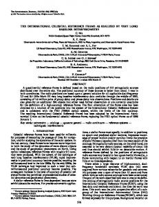
Fig. 1 Examples of two coordinate time series of non-linear sources obtained in a VLBI analysis (left) and the decomposition

low/high frequency (right).

mistakenly selected as a defining source2 (DS) for CRF and for precession-nutation. Then, using our source classification, we select several subsets of defining sources and estimate the stability of CRFs derived from the subsets’ structure. The method is inspired by Lambert (2013) [6] and explained in Section 3. The goal is to determine which criteria are predominant in the definition of a stable CRF between the behavior of the Allan Variance and the threshold value of the computed score related to the Allan Variance minima. To compare, we also add the adjustment of precession-nutation based on each CRF and study the residuals to use them as another criterion of stability. Finally, in Section 4, we draw some conclusions.

2 Contamination by Non-linear Sources From the coordinate time series from VLBI analysis, we selected some non-linear sources (NL) whose time series present variations that cannot be modeled by a 2

A defining source is how we called a source whose line-of-sight direction defines an axis of the frame.

linear function. In general, every coordinate time series can be characterized in two ways. On the one hand, we can study the high frequency components of their series composed of a thermal noise which is instrumental, of the badly modeled atmospheric component, and of the non-modeled source structure signal. On the other hand, the low frequency components gather intrinsic information about the radio center motion (e.g., periodic variations, jumps, or linear drift). So, we selected several sources that present non-linear patterns on the low frequency part of their time series in order to study their contributions to the CRF instability and to variations in the precession-nutation time series. The sources selected are 0014+813, 0528+134, 1044+719, 2145+067 (see Figure 1), 4C39.25, 0607–157 (see Figure 1), 0642+449, 0955+476, and 1739+522. In this study, all solutions produced from the adjustment of VLBI observations are based on the analysis strategy applied at Paris Observatory that produces the OPA solution3 . We only played with the subset for the no-net-rotation constraint (NNR) applied during the weighted least-squares adjustment of source coordinates. Because we compared the solutions among 3

ftp://ivsopar.obspm.fr/vlbi/ivsproducts/eops/opa2015a.eops.txt

IVS 2016 General Meeting Proceedings

294

Gattano and Lambert

Fig. 2 Annual rotations between the CRF of the reference solution (202 sources as defining sources) and annual CRFs constructed

from the CRFs of test solutions (202 − Nre jected sources as defining sources) plus the coordinate time series of the removed sources.

Fig. 3 Rotations and average coordinate differences between common sources of the CRFs from the reference solution (202 sources

as defining sources) and test solutions (202 − Nre jected sources as defining sources).

each other, the rest of the strategies are irrelevant as they are common for every solution and will thus not be detailed. We used the R1 and R4 sessions as the set of delays in our adjustments. As the reference solution, we used a solution based on a subset of the defining sources; i.e., we applied the NNR to a set of 202 VLBI sources that were observed in more than 100 sessions in the VLBI history. Then all other solutions, called test solutions, were produced by removing one of the NL listed above. A final test solution was produced by removing all NL sources plus an additional source, i.e., ten in total. When a source is rejected from the DS subset, it is adjusted locally during the analysis, i.e., with one set of coordinates for each session in which it is observed. To get an idea of the potential mistakes that an NL can bring if it is incorrectly chosen as a DS, we

computed annual coordinates of the rejected sources in each test solution. Then we computed an annual CRF for each test solution from the fixed coordinates of the DS sources to which we added the annual positions of the corresponding rejected source(s). Therefore, we got an annual CRF composed of 202 sources that we can compare to the CRF of the reference solution and get annual rotations A1 (t), A2 (t), A3 (t) for each test solution as follows: A1 tan δ1 cos α1 + A2 tan δ1 sin α1 − A3 = α1 − α2 − A1 sin α1 + A2 cos α1 = δ1 − δ2 (1) Figure 2 shows the results, and we can see that most sources have an impact of a few microseconds of arc (µas) on the CRF rotations (tens of µas for the most agitated). If you look carefully at the light blue curve


DS Selection and CRF Stability

295

Fig. 4 Differences between the precession-nutation time series obtained from the reference solution and the test solution where

0607–157 was removed from the DS subset.

corresponding to the test solution with ten sources removed from the DS subset, it appears that the value of rotations A10NL (t), A210NL (t), A10NL (t) may be the sum 1 3 NLi NLi i of the individual rotations A1 (t), ANL 2 (t), A3 (t) for all other test solutions i, with only one rejected source. That means that the effect of NL on annual CRF is additive. One can also ask if mistakingly taking out an NL source from the DS subset of the VLBI solution can affect the position of all the other sources of the DS subset. To answer this question, we took the CRFs from the test solutions, composed of 201 sources for the first nine solutions and 192 for the last, and we compared them with the reference CRF, composed of 202 sources, using Equation (1) as before but applying it to the common sources between the CRFs—that is, 201 sources (192 for the last). Figure 3 shows the results, and the effect seems negligible, less than the µas level. But, again, although small, the effect seems additive. If we took out a significant number of animated sources (e.g., one hundred) in our DS subset, the degradation in the position of the stable sources could rise to the µas level, maybe even tens of µas. Finally, what can be the effect on the precessionnutation? In our solution, we adjusted Earth Orientation Parameters (EOP) so we could compute dif-

ferences between precession-nutation from our reference solution and from the test solutions. In Figure 4, we present the example of 0607–157. The effect, at the level of hundredths of µas, is lower than the one on CRF. Therefore, to affect significantly precessionnutation by erroneously including NL in the DS subset, the amount of such mistakes should be large, even larger than the typical size of a DS subset (200∼300). But it is to be noted that the effect we see is due to the motion of the NL, because the shape of the coordinate time series is clearly recognizable in the precessionnutation difference time series.

3 Testing Allan Variance by Precession-Nutation Residuals Knowing that, with respect to Allan variance behavior, there are only 40 good sources among the 202 sources observed more than 100 times (see “Source Characterization by the Allan Variance” in these proceedings), we would like to test this classification in order to get confidence in its utilization. For this purpose we composed several DS subsets for the VLBI analysis adjustment (Table 1). The different types in the Allan Variance


296

Gattano and Lambert

Table 1 Summary of the various compositions of subsets for

defining sources (DS), standard sources (Std), and non-linear sources (NL) in several VLBI solutions. Glo=Global means the position of the source is estimated once for all sessions. Loc=Local means the position of the source is estimated for each session. NNR means we applied the no-net-rotation constraint on the corresponding source subset.

Ref. Tnt1 Tnt2 Tnt3 Twt1 Twt2 Twt3 Twt4

DS (Glo+NNR) ICRF2 DS AV0 AV0 + AV1 AV0 AV0− + AV1− + AV2− AV0− + AV1− + AV2− AV0− + AV1− + AV2− AV0− + AV1−

Std (Glo) ICRF2 Std AV1 AV0+ AV0+ + AV1+ AV2−

NL (Loc) ICRF2 NL AV2 AV2 AV1 + AV2 AV0+ + AV1+ + AV2+ AV1+ + AV2+ AV2+ AV0+ + AV1+ + AV2+

classification refer to different behaviors of the Allan Variance coordinates time series as follows: AV0

AV1

AV2

and attributes + and − refer to: p AV + ⇒ min (AVα cos δ (t)) + min (AVδ (t)) > 0.05mas p AV − ⇒ min (AVα cos δ (t)) + min (AVδ (t)) < 0.05mas Then, we got from these adjustments precessionnutation time series on which we adjusted a nutation signal from a MHB2000-based model [8] composed of 42 luni-solar principal components with corrected amplitudes to fit the adjustments plus a Free Core Nutation (FCN) signal at 430.21 days. The details of such an adjustment can be found in “The Annual Retrograde Nutation Variability” in these proceedings. Finally, we analyzed the root mean square of the residuals for both α cos δ and δ and compared their values for the different solutions. The values are displayed in Table 2. Table 2 Root mean square of the nutation residuals after adjust-

ment of an MHB2000-base model corrected to fit the results of the solution adjustment. ID Sol. Ref. Tnt1 Tnt2 Tnt3

σ (res. dX) 0.390 0.299 0.297 0.254

σ (res. dY ) 0.787 0.839 0.840 0.753

ID Sol. Twt1 Twt2 Twt3 Twt4

σ (res. dX) 0.428 0.412 0.405 0.429

σ (res. dY ) 0.799 0.804 0.809 0.800

We can see that the best residuals we got are from the solution Tnt3 where the 40 best sources with respect to Allan Variance are taken to define the axes of the CRF, and all the other sources are estimated locally. Such a result goes for a selection of stable sources from an Allan Variance point-of-view.

4 Conclusions This study is at its beginning and should be pursued to get more results and gain more confidence in what we do. At this time, we can only say that the worst non-linear sources can have an effect on the order of tens of µas if they are used by mistake in the defining sources of a VLBI solution. The consequences for the estimation of other sources are on the level of tenths of µas and at the level of hundredths of µas for the precession-nutation. But effects are additive. It means that the more mistakes we make in selecting our defining sources, the higher is the impact on astrometry and geodesy. Finally, we briefly tested our Allan Variance classification. The first results are in favor of its goodness, and we get a little more confidence in the fact that only 40 well-observed sources are currently stable.

References 1. M. Feissel-Vernier, Selecting stable extragalactic compact radio sources from the permanent astrogeodetic VLBI program, In Astronomy and Astrophysics, 2003, 403, 105–110. 2. M. Feissel-Vernier et al., Analysis strategy issues for the maintenance of the ICRF axes, In Astronomy and Astrophysics, 2006, 452, 1107–1112. 3. A.L. Fey et al., The Second Extension of the International Celestial Reference Frame: ICRF-EXT.1, In Astronomical Journal, 2004, 127, 3587-3608. 4. A.L. Fey et al., The Second Realization of the International Celestial Reference Frame by Very Long Baseline Interferometry, In Astronomical Journal, 2015, 150, 58. 5. A.M. Gontier et al., Stability of the extragalactic VLBI reference frame, In Astronomy and Astrophysics, 2001, 375, 661–669. 6. S. Lambert, Time stability of the ICRF2 axes, In Astronomy and Astrophysics, 2013, 553, A122. 7. C. Ma et al., The International Celestial Reference Frame as Realized by Very Long Baseline Interferometry, In Astronomical Journal, 1998, 116, 516–546. 8. P. M. Mathews et al., In Journal of Geophysical Research (Solid Earth), 107, 2068, 2002.
