Publisher's Disclaimer: This is a PDF file of an unedited manuscript that has been accepted for ... as the morphological signature for each voxel in deformable registration [43]. ..... and the digital errors in calculation of geodesic distance. Both of ...
NIH Public Access Author Manuscript Comput Med Imaging Graph. Author manuscript; available in PMC 2010 July 1.
NIH-PA Author Manuscript
Published in final edited form as: Comput Med Imaging Graph. 2009 July ; 33(5): 384–398. doi:10.1016/j.compmedimag.2009.03.004.
Deformation Invariant Attribute Vector for Deformable Registration of Longitudinal Brain MR Images Gang Li1, Lei Guo1, and Tianming Liu2 1 School of Automation, Northwestern Polytechnical University, Xi’an, China 2 Department of Computer Science and Bioimaging Research Center, The University of Georgia, Athens, GA, USA
Abstract
NIH-PA Author Manuscript
This paper presents a novel approach to define deformation invariant attribute vector (DIAV) for each voxel in 3D brain image for the purpose of anatomic correspondence detection. The DIAV method is validated by using synthesized deformation in 3D brain MRI images. Both theoretic analysis and experimental studies demonstrate that the proposed DIAV is invariant to general nonlinear deformation. Moreover, our experimental results show that the DIAV is able to capture rich anatomic information around the voxels and exhibit strong discriminative ability. The DIAV has been integrated into a deformable registration algorithm for longitudinal brain MR images, and the results on both simulated and real brain images are provided to demonstrate the good performance of the proposed registration algorithm based on matching of DIAVs.
1. Introduction Deformable registration of 3D brain images has been an important research area in the field of neuroimaging, and a variety of methods have been developed over the past two decades [1,3, 4,6,7,9,10,12,14,26,28,34,35,41,42]. Based on registered brain images, one can perform group or individual analysis of neuroanatomic structures to assess differences in terms of age, gender, genetic background, and handedness, etc., [2,6,24,37], to define disease-specific signatures and detect individual cortical atrophy [36,39], to automatically label and visualize cortical structure [18], to map brain function [38,39,40], or to perform neurosurgical planning [15].
NIH-PA Author Manuscript
In general, 3D brain image registration methods fall into the following two broad categories: similarity-based methods and feature-based methods. In similarity-based methods, the registration is achieved by seeking to maximize the similarity between the template image and the reference image via a deformation model, which can be based on elastic, biomechanical, fluid, or parametric approach [12,26,42]. The general similarity measures for deformable image registration could be intensity [13], mutual information [16,23,32,41], or local frequency representation [45]. In feature-based methods, anatomical feature such as surface, landmark points, or ridge are first detected in two brain images [28,43], and then a spatial transformation is used to map correspondence features. One central issue in deformable brain image registration algorithms is to develop morphological features for the detection of anatomic correspondences between the model
Publisher's Disclaimer: This is a PDF file of an unedited manuscript that has been accepted for publication. As a service to our customers we are providing this early version of the manuscript. The manuscript will undergo copyediting, typesetting, and review of the resulting proof before it is published in its final citable form. Please note that during the production process errors may be discovered which could affect the content, and all legal disclaimers that apply to the journal pertain.
Li et al.
Page 2
NIH-PA Author Manuscript
image and the subject image. Recently, several methods for defining the attribute vector with rich geometric information have been proposed, such as moment-based method [28], waveletbased method [43], and local spatial intensity histogram-based method [29]. In moment-based attribute vector method [28], MR brain images are first segmented into GM, WM, and CSF, and then the attribute vector of each voxel is extracted by computing the rotationally invariant moment feature in a spherical region for each tissue class. Since the moment-based attribute vector can be used to capture distinctive local anatomical information, it has been successfully applied to deformable volumetric MR brain image registration [28]. In the wavelet-based attribute vector method [43], the attribute vector is calculated from wavelet high-pass subimages by applying the radial profiling method. The wavelet-based attribute vector then serves as the morphological signature for each voxel in deformable registration [43]. In the local spatial intensity histogram based method [29], local spatial intensity histograms are first computed in a spherical region in each level of multi-resolution images and the attribute vector is then defined by calculating regular moment features. The local spatial intensity histogram is rotationally invariant and captures spatial information by integrating multi-resolution local histograms.
NIH-PA Author Manuscript
Although these above attribute vectors are translationally and rotationally invariant, the deformation between two longitudinal volumetric images is typically nonlinear. To address this problem, we propose a novel attribute vector that reflects the underlying anatomy and geometric information, while being deformation invariant. Deformation invariance means that the attribute vectors are the same, or very close, with the continuing homeomorphic deformation of 3D volumetric image. The deformation invariant attribute vector (DIAV) is very desirable in deformable registration of longitudinal brain images because: 1) the DIAV embodies rich geometric and intensity information of the voxel; 2) the similarity between DIAVs is a good indicator of anatomic correspondences, especially in longitudinal or timeseries brain image data, as the corresponding anatomic landmarks will have similar morphological profiles; and 3) the DIAV represents the morphological signature of a specific voxel throughout the deformation procedure and thus reduces the ambiguity in anatomic correspondence detection.
NIH-PA Author Manuscript
Our work was particularly inspired by Ling and Jacob’s method [20] for 2D image matching using geodesic intensity histogram (GIH), which is the intensity histogram of pixels extracted within a geodesic distance as deformation invariant local descriptor. We extended this work to the deformation invariant attribute vector in 3D brain images [19] and validated the method using synthesized deformations of 3D brain MR images. Our experimental studies show that the proposed DIAV achieves good deformation invariance. In addition, the DIAV embodies rich geometric and intensity information, and is quite distinctive to reduce the ambiguity in anatomic correspondence detection. Based on the matching of DIAV, a deformable registration algorithm has been developed for registration of longitudinal brain MR images. Experimental results on both simulated and real brain images are provided to demonstrate the performance of the proposed registration algorithm.
2. Method: Deformation Invariant Attribute Vector 2.1 Deformation invariant attribute for 2D images This section briefly presents the basic idea of the method introduced by Ling and Jacobs for deformation invariant 2D image matching (please refer to [20] for more details). Motivated by the Beltrami framework [31], Ling and Jacobs treated a 2D intensity image as a surface embedded in 3D space, by assigning an aspect weight α to the intensity value as the third coordinate, and weighting the first two coordinates (x and y) by 1−α. As α increases, the image deformation has less influence on the geodesic distance, which is the distance of the shortest path between two points on the embedded surface. By taking the limit of α to 1, the geodesic Comput Med Imaging Graph. Author manuscript; available in PMC 2010 July 1.
Li et al.
Page 3
NIH-PA Author Manuscript
distance becomes deformation invariant. In [20], the fast marching algorithm [27] is used to compute the geodesic distance on the embedded surface. The authors also did sampling in the geodesic distance support region (within certain geodesic level curves) to obtain deformation invariant neighborhood samples for interest points and then used a geodesic intensity histogram as deformation invariant local descriptors for 2D image matching by the χ2 distance. This method is sound in theory and achieves promising matching results in practice. 2.2 Deformation invariant attribute for 3D images In this subsection, we first extend the framework of deformation invariance in 2D space to 3D. Then, we design the deformation invariant attribute vector in 3D image using the geodesic intensity histogram. 2.2.1 3D image embedded in 4D space—We treat a volumetric image as a 3D surface embedded in 4D space. Let G (x, y, z) be a volumetric image defined as G:R3 → [0,1]. We consider the deformation as a homeomorphism between images [20], meaning that the mapping is one-to-one. Denote the embedding of an image G (x, y, z) with aspect weight α as σ(G;α) = (x′ = (1−α)x, y′ = (1−α) y, z′ = (1−α)z, g′ = αG(x, y, z)). Let γ be a regular curve on σ, and parameter p ∈ [p1, p2] (p1and p2are the boundary points). Then we have:
NIH-PA Author Manuscript
(1)
The length of curve γ is computed as:
(2)
Take the limit of α to 1: (3)
NIH-PA Author Manuscript
In the above formulas, the subscript p denotes partial derivative, e.g., xp = dx/dp, Gp = dG/dp. From Eq. (2), it is apparent that when α is large (e.g., approaching 1), it is the intensity change (represented by Gp) that dominates the length (s) of the curve γ. When taking the limit of α to 1, it is obvious that the curve length only relies on the intensity of volumetric image G, which indicates that the curve length (s) achieves deformation invariance when α → 1. 2.2.2 Geodesic distance in 3D image—As shown above, the geodesic distance between two points, which is the shortest path between them on the embedded surface, is deformation invariant when α approaches 1. Given an interest point p(x, y, z) in 3D image, the geodesic distance from it to the other points on the embedded surface σ(I;α) can be computed using the fast marching algorithm [27]. The fast marching method was developed to effectively solve the problem of front propagation, involving computing a new position of an initial curve when a force F is applied. A function T denotes the time when the curve reaches a position, and the Eikonal equation governs the curve propagation:
Comput Med Imaging Graph. Author manuscript; available in PMC 2010 July 1.
Li et al.
Page 4
(4)
NIH-PA Author Manuscript
where ∇T is the gradient of T. In our application, we use the extended fast marching method in 3D image in [8]. To compute the geodesic distance, the parameter T in the Eq. (4) is set as the geodesic distance, and the marching speed F is set to:
(5)
where the subscripts (x, y and z) denote partial derivatives. Figure 1 shows a color-coded geodesic distance map from a selected voxel (marked with a red cross) to other voxels in a volumetric MR brain image. Here, the red color indicates small geodesic distance, while blue color indicates large geodesic distance. For convenient visual inspection, we only show selected 2D orthogonal slices. In the example, α is set to be 0.98. Evidentally, the geodesic distance in 3D image can be used to capture the geometry of image intensities.
NIH-PA Author Manuscript
2.2.3 Deformation invariant attribute vector—As both the geodesic distance (when α → 1) and intensity are deformation invariant, we can use geodesic distance histogram to define deformation invariant attribute vector (DIAV). Given an interest voxel p, along with neighboring voxels in the geodesic distance support region, the geodesic intensity histogram (GIH) is calculated as follows. We divide the intensity and geodesic distance space into K×M bins. Let {xi}i=1…n be the voxel locations in the geodesic distance region. The function v : R3 → {1…K} maps the voxel at location xi to the index v(xi) of its bin in the quantized intensity space. The function g:R3 → {1…M} maps the voxel at location xi to the index g(xi) of its bin in the quantized geodesic distance space. The GIH at k = 1…, m = 1…M is computed as:
(6)
NIH-PA Author Manuscript
where δ is the Kronecker delta function. After computing the GIH, we normalize each column of Hp at the same geodesic distance, and then normalize the whole Hp. It should be noted that, when computing GIH, we do not need to compute the geodesic distances from a study voxel to all of the others, but rather compute geodesic distances from the voxel to those voxels within a geodesic threshold, all of which define the support region. Figure 2 shows an example of geodesic distance support region for calculating geodesic intensity histogram from a voxel indicated by a red cross in volumetric MR brain image. Here, the color-coded geodesic distance support region is overlaid on the axial, coronal and sagittal slices respectively. The 3D volume rendering of the support region is also displayed in three views. The support region for the calculation of GIH is clearly an irregular and complicated volume. This complicated support region helps the GIH capture rich geometric and anatomic information, which renders distinctiveness of the GIH to reduce the ambiguity in correspondence detection. With the geodesic intensity histogram in 3D image, we define a deformation invariant attribute vector (DIAV) H(x) for each voxel by concatenating every column (in the same geodesic distance bin) in the geodesic intensity histograms as:
Comput Med Imaging Graph. Author manuscript; available in PMC 2010 July 1.
Li et al.
Page 5
(7)
NIH-PA Author Manuscript
As the geodesic intensity histogram is deformation invariant, the DIAV is deformation invariant. To compare DIAVs, we define the similarity of two DIAVs (H(x) and H(y)) of two voxels (x and y) as follows:
(8)
where Hx(i) is the i-th element in H(x).
3. Method: Deformable Registration based on DIAV Matching 3.1 Formulation
NIH-PA Author Manuscript
The deformable registration algorithm is formulated as an energy minimization problem [33]. Specifically, the external energy is to maximize the similarity of the DIAVs of voxels in the model and that in the subject respectively. The internal energy function term serves as a smoothness constraint on the displacement fields, similar to those in [21] and [28]. The energy function is defined as follows:
(9)
where and are external and internal energy terms, defined for the voxel v in the model image. wExt and wInt are weighting parameters. The goal of registration is to deform the model image VMdl to the subject image VSub, using the DIAV matching method. That is, for each model voxel v in the volume VMdl, we seek its correspondence in the subject image VSub. If the correspondence is successfully determined, the volume neighborhood N(v) around the model voxel v will be deformed to the subject image by a local transformation Tv. Therefore, the transformation h in the registration is decomposed into a number of local transformations {Tv}, i.e., h = Tv}.
NIH-PA Author Manuscript
The external energy term measures the DIAV similarity of the voxel in the model and that in the subject image, respectively. It requires that the DIAV of the neighboring voxel vj in the volume neighborhood N(v) be similar to that of its counterpart in the subject volume, and vice versa. The mathematical definition is given as:
(10)
where p(.) denotes the projection of a point to the closest voxel in the volume, since the transformed point Tv(vj)or is not necessary on the volume voxel. is the reverse transformation of Tv (.). The definition of similarity m(.) is referred to Eq. (8). ϖT and ϖR are weighting terms for forward and reverse transformation. The internal energy term
designed to preserve the smoothness of the deformation field:
Comput Med Imaging Graph. Author manuscript; available in PMC 2010 July 1.
Li et al.
Page 6
NIH-PA Author Manuscript
(11)
where Uvj is the coordinate of voxel vj. We use a greedy deformation algorithm [21,28] to minimize the energy function stated in Eq. (9). We deform the voxels within a small neighborhood around each model voxel, rather than deforming only the model voxel. This decreases the probability of being trapped in local minima. Notably, before the registration procedure, both model and subject images are pre-processed using the tools described in [21] and [22]. 3.2 Hierarchical energy minimization
NIH-PA Author Manuscript
It has been shown that performing voxel-wise feature matching for the whole volume is timeconsuming and has a high risk of being trapped in a local minimum [21,28]. A desirable solution thus is to select the most important voxels to drive the registration hierarchically. The idea is that, initially, the volume deformation is driven by a small fraction of selected voxels, which usually have more distinctive attribute vectors, and are less prone to the risk of being trapped in local minimum. In the following deformation, the dimensionality of the energy function is increased by involving more hierarchically selected voxels. In this paper, we used a similar hierarchical driving voxels selection scheme as introduced in [28]. Figure 3 provides an example of the hierarchical driving voxel selection procedure. 3.3 Adaptive deformation There might be structure changes in volumetric time-series images, thus resulting in fundamental morphological differences between the template and the subject. In such cases, the registration algorithm relaxes the matching forces when no good matching is found, and the deformations on such structures will be driven primarily by the deformations of the voxels in the neighboring structures with higher confidence. This adaptive deformation scheme based on the confidence level is akin to those in [5] and [21], which emphasizes the importance of measuring the degree, regional variation, and confidence in the correspondences established by image registration. Here, the DIAV similarity map is used as the confidence map to guide the adaptive deformation scheme. 3.4 Consistent transformation
NIH-PA Author Manuscript
The concept of consistent image registration was introduced in [11], meaning that the registration gives the same mapping between two images no matter which one is treated as the template. The constraint of consistent transformation in the registration algorithm renders more robustness to local minima as demonstrated by a variety of publications in the literature [28]. In this paper, we use the symmetric external energy function term in Eq. (10) to implement the constraint of inverse consistent transformation.
4. Experimental Results A series of experiments are conducted to evaluate the DIAV and the proposed registration algorithm. Both synthesized brain images and real brain images are used to demonstrate the performance of the proposed algorithms. 4.1 Experimental results on DIAV Evaluation studies are performed to examine the performance of DIAV. In the first experiment, we demonstrate the deformation invariance of DIAV by using synthesized volumetric image
Comput Med Imaging Graph. Author manuscript; available in PMC 2010 July 1.
Li et al.
Page 7
NIH-PA Author Manuscript
deformation. In the second experiment, we demonstrate the discriminative ability of DIAV. In the third experiment, we compare the DIAV with the wavelet-based attribute vector [43] and local spatial intensity histogram [29]. Finally, we investigate the relationship between the deformation invariance and geodesic distance threshold, and the computational cost in calculating DIAV. In all these experiments, we used twelve 3D T1 SPGR images of normal human brains. Before computing DIAV, we have normalized the intensities of all the images to the range of [0, 1]. In order to convert anisotropic images to isotropic ones, we interpolate the images bilinearly and re-sample the images. The re-sampled voxel size is 0.94 mm in three directions, and the re-sampled image size is 256×256×198. 4.1.1 Examination of the deformation invariance of DIAV
NIH-PA Author Manuscript
4.1.1.1 Examination via synthesized inter-subject deformation: We have shown in theory that the DIAV is deformation invariant in Section 2.2. Here, we demonstrate that the DIAV is deformation invariant by using synthesized brain image deformation. To obtain synthesized 3D inter-subject image deformation, we manually painted major sulci on the model and individuals, and used them as constraints to warp the model into individuals using an elastic warping algorithm [7]. Additional details of the procedure are referred to [21,28]. With the synthesized 3D brain image deformation, we know the exact correspondence of the voxels in the original image and the deformed one. For a pair of corresponding voxels in these two images, we calculate their DIAVs and compare their similarity as defined in Eq. (8). To visually illustrate the deformation invariance of the GIH, Figure 4 shows an example of geodesic intensity histograms of a pair of correspondence voxels in the original MR brain image and the synthesized deformed image. The two geodesic intensity histograms are quite similar to each other, with the similarity of 0.93, although the deformation around the voxel is large and nonlinear.
NIH-PA Author Manuscript
As an example, we randomly selected one pair of the original image and the deformed one. In the original image, we randomly picked fifty voxels in the same slice for the convenience of visualization, as shown in Figure 5a. Then we compare the similarities of the DIAVs of the voxels in the original image and those in the deformed one. Figure 5b shows the DIAV similarities for the selected fifty voxels. The highest DIAV similarity is 0.99, and the lowest DIAV similarity is 0.91. The average DIAV similarity over the fifty cases is 0.95, and the standard deviation is 0.025. These high similarities indicate that the DIAV has good performance of being deformation invariant, considering that the average length of the deformation vectors of the fifty voxels is 7.1 mm. The lengths of the deformation vectors of the 50 voxels are shown in Figure 5c. The data in Figure 5 show that no matter how large the deformation is (ranging from 3.3 mm to 12.6 mm), the DIAV similarities are constantly over 0.9. We have performed similar experiments in the other eleven pairs of original images and deformed images, and achieved similar results. The average similarity of the DIAVs of the voxels in the twelve original image pairs and the deformed ones is 0.95. These results further demonstrate that the proposed DIAV is deformation invariant. To examine DIAV more extensively, we computed the similarities between the voxels in the selected slice shown in Figure 5 and their corresponding voxels in synthesized deformed image. Figure 6a displays the distribution of the DIAV similarities of all the voxels in the slice, with the average similarity of 0.929, given that the average length of deformation vectors is 6.50 mm. Figure 6b shows the deformation vector length histogram for all the voxels in the slice. The results in Figure 6 apparently demonstrate that the DIAV is deformation invariant for synthesized inter-subject deformation. Notably, image voxels closer to tissue boundaries have relatively lower DIAV similarities. This is because these voxels are more sensitive to the interpolation errors in image warping and the digital errors in calculation of geodesic distance. Both of these errors are inevitable in Comput Med Imaging Graph. Author manuscript; available in PMC 2010 July 1.
Li et al.
Page 8
NIH-PA Author Manuscript
practical implementations of the DIAV algorithms. To compare the difference of DIAV performance in gray matter and white matter regions, we compute the average similarity of DIAVs of all the voxels in a randomly selected slice. The average similarity for GM and WM regions are 0.90 and 0.95 respectively. 4.1.1.2 Examination via simulated intra-subject deformation: We used a biomechanical model to simulate the mass effect caused by a growing tumor, which is akin to the method in [17]. The tumor growth is driven by the boundaries of a manually placed brain tumor seeds, which expand spherically. The deformation of the surrounding tissue is estimated using a nonlinear elastic model of soft tissue [17,25]. Figure 7a and 7b show the original brain image with manually placed tumor seeds and the deformed image after tumor growth. Then the simulated intra-subject deformation is used as ground truth to evaluate the DIAVs in the original and deformed images.
NIH-PA Author Manuscript
For visual inspection, we randomly selected fifteen points in the vicinity of the simulated brain tumor image (shown in Figure 7a), and compute the similarities between the DIAVs of those points in the original and deformed images. Figure 7c is the DIAV similarity result of the fifteen points. The average similarity over the fifteen cases is 0.935, given that the average length of the deformation vectors of the fifteen voxels is 3.4 mm. The lengths of the deformation vectors of the fifteen voxels are in Figure 7d. These results indicate that DIAV has good performance of being deformation invariant given nonlinear intra-subject deformation. To examine the DIAVs for intra-subject deformation more extensively, we select all the voxels located between two spheres around the tumor seed region, as shown in Figure 8a. The radii of the two spheres are 8 mm and 13 mm respectively, thus totally involving 6,101 voxels in the ring region. Then we compute the similarities of the DIAVs of the voxels in the original image and the corresponding voxels in the deformed image. Figure 8b shows the distribution of the DIAV similarities of all the voxels in the ring region, with the average similarity of 0.934, given that the average length of deformation vectors is 3.02 mm. Figure 8c shows the deformation vector length histogram for all the voxels in the ring region. The results in Figure 8b and Figure 8c clearly demonstrate that the DIAV is deformation invariant for intra-subject deformation, and has wide potential applications in the registration of longitudinal brain images.
NIH-PA Author Manuscript
4.1.2 Examination of the discriminative ability of DIAV—A key objective in designing the attribute vector for brain image registration is that the attribute should represent the morphological information of a voxel as rich as possible and should discriminate fine, local anatomic structures [21,28]. In this experiment, we evaluate the discriminative ability of DIAV. If the DIAV, representing the morphological signature of a voxel throughout the deformation procedure, can be used to capture rich image content in distinguishing one voxel from the others, then it can be used for effective detection of anatomical correspondences in deformable registration of 3D brain images. One means to evaluate the morphological richness of an attribute is to compare the attribute of a voxel with those of its neighbors. If the attribute vector can distinguish the voxel from the others, it is considered morphologically rich [21,28]. Our experiments show that the proposed DIAV is quite distinctive in discriminating the voxel of interest from the other voxels. As an example, Figure 9a and 9b show the DIAV similarities between a randomly selected voxel A with its neighbors. To better visualize the result, the vicinity region of the voxel is zoomed. The dark red peak around the interest voxel apparently demonstrates the distinctiveness of the DIAV of voxels. To examine the discriminative ability of DIAV in correspondence detection, a voxel located in white matter area is randomly selected (B in Figure 9c). Its correspondence voxel B′ in the synthesized image is shown Figure 9d. Figure 9e presents the DIAV similarity
Comput Med Imaging Graph. Author manuscript; available in PMC 2010 July 1.
Li et al.
Page 9
NIH-PA Author Manuscript
map between B and all the voxels in Figure 9d. The dark red area around the voxel B′ apparently demonstrates the good distinctiveness of the DIAV. Figure 9f shows the DIAV similarity map between voxel B′ and all of the voxels in the image of Figure 9d. The dark red area around voxel B′ in Figure 9f demonstrates the discriminative ability of DIAV for voxels that share a similar anatomical environment. To analyze the discriminative ability quantitatively, we compute the average of the DIAV similarity between a voxel and other voxels in a series of ring regions centered on the voxel. The thickness of each ring is set to be one voxel, with the radius ranging from 1 to 10 voxels. Nine different geodesic distance thresholds are used, ranging from 0.2 to 1.0 with an interval of 0.1. Figure 9g shows the similarity curve along the radius of ring for each geodesic distance threshold averaged over multiple randomly selected voxels. Here, the similarity decreases rapidly with the increasing of the radius of ring regions. 4.1.3 Comparison of DIAV with SIH and WAV—To demonstrate the advantage of the deformation invariant attribute vector, we compare the DIAV with the local spatial intensity histogram (SIH) [29] and the wavelet-based attribute vector (WAV) [43] in terms of their deformation invariance properties.
NIH-PA Author Manuscript
4.1.3.1 Calculation of SIH and WAV: For SIH, we first down sample the original image by a sampling factor of two, resulting in three resolution level images. Then we compute the local intensities histogram in a spherical region of each point in each resolution image. We set the radius of the spherical regions to 8 mm, 4 mm, and 4 mm in the three resolution levels. As a result, we have three local histograms for each voxel in the original image. Finally, we calculate the moment features for each local histogram respectively, which is akin to [29]. More details of SIH are referred to [29]. Similar definition of attribute vector similarities as in Eq. (8) is used for SIH. Notably, before calculating the similarity between two SIHs, we normalize each element of attribute vector between 0 and 1. For WAV, three resolution levels of images are used. The sliding window size is set to 8 mm for the lowest level, 4 mm for the middle and the highest resolution. Two-level DWT decomposition is performed to calculate the wavelet subimages at each resolution level. The length-1 Daubechies wavelet is used to calculate the DWT sub-images, see [43] for more details of WAV. Similarly, each element of the attribute vector is normalized between 0 and 1, and a similar definition of attribute vector similarities as in Eq. (8) is used for WAV.
NIH-PA Author Manuscript
4.1.3.2 Comparison of deformation invariance and distinctiveness: To evaluate the deformation invariance properties of SIH and WAV, Figure 10a shows the attribute similarities between the randomly selected fifty voxels in Figure 5a and their corresponding voxels in the deformed image for SIH and WAV. The details of the deformation simulation are referred to Subsection 4.1.1. The average similarity of SIH and WAV are 0.59 and 0.76, which are much lower than that for DIAV (0.95). This is expected as the SIH and WAV are defined in a spherical region, which is only invariant to rotation. To compare the SIH and WAV with the DIAV more extensively, Figure 10b displays the distribution of the SIH and WAV similarities of all the voxels in the slice in Figure 5a. The average similarities of SIH and WAV are 0.83 and 0.73, which are much lower than that for DIAV (0.929), as shown in Figure 6a. To analyze the discriminative ability of SIH and WAV quantitatively, we compute the average of the DIAV similarity between a voxel and other voxels in a series of ring regions centered on the considered voxel. Figure 10c shows the similarity curve along the radius of ring averaged over the multiple randomly selected voxels. Although the similarity decreases with the increasing of the radius of ring regions, its discriminative ability is not as good as that of DIAV, as shown in Figure 10c.
Comput Med Imaging Graph. Author manuscript; available in PMC 2010 July 1.
Li et al.
Page 10
NIH-PA Author Manuscript
4.1.4 Deformation invariance and geodesic distance threshold—The geodesic distance threshold, which determines the support region for DIAV calculation, has direct influence on the performance of DIAV’s deformation invariance. In order to analyze the relationship between geodesic distance threshold and the DIAV’s deformation invariance, we set ten different geodesic distance thresholds, ranging from 0.1 to 1.0 with interval of 0.1, to calculate DIAVs. We use the same selected voxels from twelve volumetric brain MRI images as in Subsection 4.1.1. For each geodesic distance setting, we compute the average similarity of the DIAVs of these voxels in the original image and the deformed one. Figure 11 displays the average similarity of DIAVs with varying geodesic distance thresholds. There exists a similarity peak of 0.97 when the geodesic distance threshold is 0.2. The average similarity of DIAVs descends slowly with the geodesic distance threshold increasing from 0.3 to 1.0. The average similarity, however, is still very high, consistently larger than 0.91. Our explanation to this phenomenon is that the larger geodesic distance threshold is, the more image voxels are involved and the more computational and digital errors exist in the calculation of DIAV. On the contrary, when the geodesic distance is less than 0.2, it is too small to capture sufficient number of voxels to keep the calculation of DIAV stable, resulting in lower average similarity of DIAVs.
NIH-PA Author Manuscript
4.1.5 Computational cost and geodesic distance threshold—As seen in Section 2, the computation time of deformation invariant attribute vector rely on the size of the selected geodesic distance support region. The larger of the support region is, the more geodesic distances from the selected voxel to the other voxels need to be computed and the more computation time is consumed. The bottleneck of calculating DIAV is the step of computing geodesic distance via fast marching method. To investigate the running time, we set ten different geodesic distance thresholds, ranging from 0.1 to 1.0, for calculating DIAVs. We tested hundreds of voxel selected from 12 volumetric brain MRI images. All of the experiments are carried out on a standard PC (Intel Pentium IV 2.4 Ghz) using C/C++ implementation. Figure 12 shows the average time of calculating DIAV for one voxel with varying geodesic distance thresholds. The running time grows rapidly as the geodesic region threshold increases, e.g., when the geodesic distance threshold approaches 1.0, the running time is around 12 ms for calculating one DIAV. That means it is impractical to compute the DIAVs for all of the voxels in the whole volumetric image when geodesic distance threshold is set to be large (close to 1.0) with our current DIAV implementation. 4.2 Result of registration algorithm on synthesized brain images
NIH-PA Author Manuscript
We use the same thirteen synthesized brain images obtained by the method in Subsection 4.1.1 to evaluate the performance of the registration method. For the synthesized images, we know the exact correspondence between the voxels in the template and subject images. In this way, we can directly compare the registration errors that occur in the registration method. As shown in Figure 13, we use the histogram of registration errors to display the registration performance. For these two cases, the average registration errors are 0.91 and 0.92, and the maximum registration errors are 4.53 and 3.61 respectively. Table 1 shows the average and maximum registration errors for these thirteen cases. For visual inspection of the registration error, Figure 14b presents the color-coded registration error for one slice in the first case, most areas of the slice have quite low registration errors (blue). Figure 14c compares the average image of the thirteen synthesized images warping onto the model image with the original model image. The average image is apparently clear, indicating the registration for all of the thirteen images is quite accurate.
Comput Med Imaging Graph. Author manuscript; available in PMC 2010 July 1.
Li et al.
Page 11
4.3 Result of registration algorithm on real brain images
NIH-PA Author Manuscript
This experiment shows the results of quantifying the deformation induced by the growth of a tumor, captured by serial intra-patient images as shown in Figure 15. These serial images were scanned with the same T1 SPGR imaging protocol of the same patient with brain glioma tumor at approximately half-year intervals. In order to estimate the tumor deformation from time point 1 to time point 5, we used the proposed registration method to directly register the images of time points 1 to 5. To quantitatively evaluate the proposed algorithm in registering serial scans, we measured the registration errors on manual landmarks defined by two human raters in the images of timepoints 1 and 5. Two representative pairs of corresponding landmarks are shown in Figures 15. Since the two images of time-points 1 and 5 have been rigidly aligned before placing manual landmarks, the distance between each manual landmark in the image of time-point 1 and its corresponding landmark in the image of time-point 5 indicates the displacement or deformation at that location, measured by manual raters, due to the mass effect of the growing tumor. Figure 16a shows the displacement on each landmark obtained by two raters for one case. The average displacement over the twenty landmarks is 5.43 mm, which indicates quite a large deformation induced by tumor growth, particularly since the deformation was significantly larger very close to the tumor.
NIH-PA Author Manuscript
We measured the displacement estimation error of our algorithm on these twenty landmarks. As shown in Figure 16a, the average estimation error compared with the first rater is 1.21 mm. As for the evaluation results by the second rater, the average registration error is 1.21 mm. These results demonstrate that the displacements/deformation due to tumor growth can be captured by the proposed registration algorithm with relatively good accuracy, compared to the average inter-rater difference of 1.22 mm. For the purpose of comparison, we performed direct correspondence voxel detection in the time-point 5 image, given the manually-labeled landmarks in the time-point 1 image. Their correspondence voxels in the time-point 5 image are defined as the voxels that have the most similar DIAVs. The direct correspondence detection result is reasonably good, as shown in Figure 16b, though it is less accurate than the registration result in Figure 16a by around 34%.
NIH-PA Author Manuscript
Figure 17 presents the result for the second case of serial intra-patient images. In this case, the average displacement of twenty landmarks is 4.26 mm, the average registration errors compared with two raters are 1.13 mm and 1.24 mm respectively, and the inter-rater difference is 1.08 mm (Figure 17a). These results further demonstrate that the proposed registration algorithm has good accuracy compared to expert raters. In comparison, the direct correspondence detection by the maximization of DIAV similarity is less accurate than the registration algorithm by about 23% for the 20 landmarks (Figure 17b).
5. Discussion and Conclusion 5.1 Selection of alpha Alpha, which controls the aspect weight, is a critical parameter for obtaining the geodesic support regions. When alpha is close to 1, the DIAV feature should be deformation invariant in theory. On the other hand, when alpha is close to 0, the feature should be only rotation invariant instead of being deformation invariant. Here, we select several sampling discrete values of alpha between 0 and 1, and evaluate how alpha influences the deformation invariance of DIAV, which is measured by the similarity of corresponding DIAVs in synthesized brain MR images in section 4.1. Figure 18 shows the curve of average similarities varying with alpha. As shown in Figure 18, when alpha is set to be 0, the average similarity of DIAVs is around 0.85. As alpha increases from to 0.98, the average similarity becomes to be around 0.93. There Comput Med Imaging Graph. Author manuscript; available in PMC 2010 July 1.
Li et al.
Page 12
NIH-PA Author Manuscript
is no obvious change between alphas setting to be 0.98 and 0.99. Our explanations to the phenomenon are: when alpha is 0, DIAVs are only rotation invariant. This level of average similarity (0.85) is close to that of SIH in Section 4.1.3. As alpha increases to 0.98, DIAVs tend to be invariant to general nonlinear deformations. This is the reason that we select the value of alpha as 0.98 in all of the registration experiments. Notably, smaller alpha might be good enough for some regions with smaller nonlinear deformations. Currently, we do not know which areas have relatively small nonlinear deformations and which areas have relatively large nonlinear deformations. In the future, we intend to adopt machine learning based method (e.g., in [44]) to learn the prior knowledge of the distribution map of deformation magnitude. Then we can assign appropriate alpha in different regions. In addition, we could gradually change the value of alpha along with the iterations of the registration procedure. At the initial stage of registration, the nonlinear deformation between two volume images is larger, so relatively larger alpha should be chosen in order to deal with larger nonlinear deformations. Whereas along with the iterations of registration, the nonlinear deformation magnitude is reduced gradually, therefore smaller alpha should be enough to cope with small nonlinear deformation. 5.2 Sensitivity to noise and intensity inhomogeneity
NIH-PA Author Manuscript
Noise and intensity inhomogeneity are inevitable in the acquisition of brain MR image. To reduce the influence of noise and intensity inhomogeneity on the registration result, several steps are performed as follows. Firstly, brain MR images are smoothed to reduce noises. Then, in order to deal with the intensity inhomogeneities, the N3 method [30] is used to correct the intensity inhomogeneities in each image. Finally, to make the distributions of the two intensity histograms globally similar, then the histogram of one image is linearly transformed to match the histogram of the other, which is similar to the method employed in [29] for intensity based elastic registration. To examine the ability of above steps in dealing with the noise and intensity inhomogeneities, we added multiplicative biased field and additive Gaussian white noise to the synthesized brain images, as shown in Figure 19a as an example. Then, we compare the registration result by the proposed methods with the ground-truth. The average registration difference is: 0.03 mm. The relatively small difference indicates that the proposed registration method is not sensitive to noise and intensity inhomogeneities. In the future, we plan to adopt the histogram similarity measure as described in [20], which is based on the fact that the diffusion distance is more robust to intensity change and noise in histogram-based local descriptors. This new definition of DIAV similarity using diffusion distance between histograms might be able to further improve the robustness of DIAV to noises. 5.3 Computational time
NIH-PA Author Manuscript
Our current implementation of the registration algorithm takes about 2.7 hours (Intel Pentium IV 2.4 Ghz and 2 GB memory), including 1.5 hours for DIAV computing and 1.2 hours for deformable registration. The computational time is comparable to existing nonlinear registration methods (e.g., [28]). Our future work will optimize the implementation for both DIAV computing and deformable registration to speed up the system. In addition, the calculation of each DIAV does not rely on other DIAVs, meaning that the procedure of DIAV computing can be accelerated in parallel in the future.
5.4 Conclusion This work contributes a novel method that defines deformation invariant attribute vector for 3D brain images to achieve automatic correspondence determination. Extensive experiment results reported in this paper have shown that the proposed DIAV achieves good deformation invariance. Furthermore, the DIAV, which represents the morphological signature of a voxel throughout the deformation procedure, has good discriminative capability and thus can reduce the ambiguity in the determination of anatomic correspondences. These advantages motivated
Comput Med Imaging Graph. Author manuscript; available in PMC 2010 July 1.
Li et al.
Page 13
NIH-PA Author Manuscript
us to integrate the DIAV into a deformable registration algorithm for longitudinal brain MR image studies. Experimental results on both synthesized and real brain images have demonstrated the reasonably good performance of the registration algorithm based on DIAV matching. The proposed registration algorithm for longitudinal volumetric images has potential applications in: 1) quantification of chronic disease progression for computer aided diagnosis and prognosis, e.g., serial measurements of regional brain morphology via MRI in neurodegenerative and other neurological disease; and 2) quantification of patient response to therapy via computer aided follow-up, e.g., measurement of tumor morphology using MRI to evaluate the effect of stereotactic radiosurgery and measurement of tumor size and metabolism to evaluation tumor progression or response following chemotherapy. Our future work plans to apply this registration algorithm in clinical applications of measuring longitudinal changes of neuroanatomic structures in brain diseases.
Acknowledgements
NIH-PA Author Manuscript
G Li and L Guo were supported by the Northwestern Polytechnical University Foundation for Fundamental Research. T Liu was supported by the NIH Career Award (EB-006878) and the University of Georgia start-up research funding. We would like to express our appreciation to Dr. Dinggang Shen and Dr. Christos Davatzikos for sharing the HAMMER software package and the associated datasets, and thanks to Dr. Nick Fox for sharing the serial intra-patient brain tumor images and to Dr. Geoffrey Young and Dr. Stephen TC Wong for helpful discussions. Finally, we would like to thank Dr. Ashraf Mohamed who helped to manually label the landmarks in Section 4.3, and thank Dr. Haibing Ling who provided helpful discussions and feedback to the work presented in this manuscript.
References
NIH-PA Author Manuscript
1. Ashburner J, Friston KJ. Multimodal image coregistration and partitioning: a unified framework. NeuroImage 1997;6(3):209–217. [PubMed: 9344825] 2. Ashburner J, Csernansky JG, Davatzikos C, Fox NC, Frisoni GB, Thompson PM. Computer-assisted imaging to assess brain structure in healthy and diseased brains. Lancet Neurology 2003;2(2):79–88. [PubMed: 12849264] 3. Bajcsy R, Lieberson R, Reivich M. A computerized system for the elastic matching of deformed radiographic images to idealized atlas images. Journal of Computer Assisted Tomography 1983;7(4): 618–625. [PubMed: 6602820] 4. Collins DL, Neelin P, Peters TM, Evans AC. Automatic 3D inter-subject registration of MR volumetric data in standardized Talairach space. Journal of Computer Assisted Tomography 1994;18(2):192–205. [PubMed: 8126267] 5. Crum WR, Griffin LD, Hill DLG, Hawkes DJ. Zen and the art of medical image registration: correspondence, homology, and quality. NeuroImage 2003;20:1425–1437. [PubMed: 14642457] 6. Davatzikos C, Bryan N. Using a deformable surface model to obtain a shape representation of the cortex. IEEE Transactions on Medical Imaging 1996;15(6):785–795. [PubMed: 18215958] 7. Davatzikos C. Spatial transformation and registration of brain images using elastically deformable models. Computer Vision and Image Understanding 1997;66(2):207–222. [PubMed: 11543561] 8. Deschamps T, Cohen LD. Minimal Path in 3D Images and Application to Virtual Endoscopy. ECCV. 2000 9. Evans AC, Dai W, Collins L, Neeling P, Marett S. Warping of a computerized 3-D atlas to match brain image volumes for quantitative neuroanatomical and functional analysis. SPIE Procedding, Image Processing 1991;1445:236–246. 10. Fischl B, Sereno MI, Tootell R, Dale AM. High-resolution intersubject averaging and acoordinate system for the cortical surface. Human Brain Mapping 1999;8:272–284. [PubMed: 10619420] 11. Christensen, GE. Consistent Linear-Elastic Transformations for Image Matching. Information Processing in Medical Imaging, LCNS 1613; Springer-Verlag. 1999. p. 224-237.
Comput Med Imaging Graph. Author manuscript; available in PMC 2010 July 1.
Li et al.
Page 14
NIH-PA Author Manuscript NIH-PA Author Manuscript NIH-PA Author Manuscript
12. Gee JC, Barillot C, Briquer LL, Haynor DR, Bajcsy R. Matching structural images of the human brain using statistical and geometrical image features. Proc SPIE Visualization in Biomedical Computing 1994;2359:191–204. 13. Johnson H, Christensen G. Consistent landmark and intensity-based image registration. IEEE Trans Med Imaging 2002;21(5):450–461. [PubMed: 12071616] 14. Joshi SC, Miller MI, Christensen GE, Banerjee A, Coogan T, Grenander U. Hierarchical brain mapping via a generalized Dirichlet solution for mapping brain manifolds. Proceedings of the SPIE Conference on Geometric Methods in Applied Imaging 1996;2573:278–289. 15. Kikinis R, Jolesz FA, Lorensen WE, Cline HE, Stieg PE, Black P. 3D reconstruction of skull base tumors from MRI data for neurosurgical planning. Proceedings of the Society of Magnetic Resonance in Medicine Conference. 1991 16. Kjems U, Strother SC, Anderson J, Law I, Hansen LK. Enhancing the multivariate signal of [15O] water PET studies with a new nonlinear neuroanatomical registration algorithm. IEEE Trans Med Imaging 1999;18(4):306–319. [PubMed: 10385288] 17. Kyriacou SK, Davatzikos Christos, Zinreich SJ, Bryan RN. Nonlinear elastic registration of brain images with tumor pathology using a biomechanical model. IEEE Trans Med Imaging 1999;18(7): 580–592. [PubMed: 10504092] 18. Le Goualher G, Procyk E, Collins L, Venegopal R, Barillot C, Evans A. Automated extraction and variability analysis of sulcal neuroanatomy. IEEE Transactions on Medical Imaging 1999;18:206– 216. [PubMed: 10363699] 19. Li, Gang; Liu, Tianming; Young, Geoffrey; Guo, Lei; Wong, Stephen TC. Deformation invariant attribute vector for 3D medical image registration. International Symposium on Biomedical Imaging; Washington DC. 2006. 20. Ling, H.; Jacobs, DW. Deformation Invariant Image Matching. ICCV; 2005; Beijing, China. 2005. 21. Liu T, Shen D, Davatzikos C. Deformable registration of cortical structures via hybrid volumetric and surface warping. NeuroImage 2004;22(4):1790–1801. [PubMed: 15275935] 22. Liu T, Young G, Huang L, Chen NK, Wong S. 76-space Analysis of Grey Matter Diffusivity: Methods and Applications, NeuroImage 2006;31(1) 23. Maes F, Collignon A, Vandermeulen D, Marchal G, Suetens P. Multimodality image registration by maximization of mutual information. IEEE Trans Med Imaging 1997;16(2):187–198. [PubMed: 9101328] 24. Mangin, JF.; Rivière, D.; Cachia, A.; Papadopoulos-Orfanos, D.; Collins, DL.; Evans, AC.; Régis, J. Object-based strategy for morphometry of the cerebral cortex. IPMI; Ambleside, UK. 2003b. 25. Mohamed, A.; Davatzikos, C. Finite element mesh generation and remeshing from segmented medical images. ISBI 2004; Arlington, VA. 2004. 26. Rueckert D, Sonoda LI, Hayes C, Hill DLH, Leach MO, Hawkes DJ. Nonrigid registration using free-form deformations: Application to breast MR images. IEEE Trans Med Imaging 1999;18(8): 712–721. [PubMed: 10534053] 27. Sethian JA. A fast Marching Level Set Method for Monotonically Advancing Fronts. Proc Natl Acad Sci 1996;93:1591–1595. [PubMed: 11607632] 28. Shen D, Davatzikos C. HAMMER: Hierarchical Attribute Matching Mechanism for Elastic Registration. IEEE Trans Med Imaging 2002;21(11):1421–1439. [PubMed: 12575879] 29. Shen, D. Image Registration by Hierarchical Matching of local Spatial Intensity Histograms. MICCAI 2004; France. 2004. 30. Sled JG, Zijdenbos AP, Evans AC. A non-parametric method for automatic correction of intensity non-uniformity in MRI data. IEEE Transactions on Medical Imaging 1998;17(1):87–97. [PubMed: 9617910] 31. Sochen N, Kimmel R, Malladi R. A General Framework for Low Level Vision. IEEE Trans Image Processing 1998;7(3):310–318. 32. Studholme C, Hill DLG, Hawkes DJ. An overlap invariant entropy measure of 3D medical image alignment. Pattern Recognition 1999;32(1):71–86. 33. Terzopoulos D, Fleischer K. Deformable models. The Visual Computer 1988;4(6):306–331.
Comput Med Imaging Graph. Author manuscript; available in PMC 2010 July 1.
Li et al.
Page 15
NIH-PA Author Manuscript NIH-PA Author Manuscript
34. Thirion JP, Monga O, Benayoun S, Gueziec A, Ayache N. Automatic registration of 3-D images using surface curvature. SPIE Proc, Mathematical Methods in Medical Imaging 1992;1768:206–216. 35. Thompson PM, Toga AW. A surface-based technique for warping 3-dimensional images of the brain. IEEE Transactions on Medical Imaging 1996;15:1–16. 36. Thompson PM, Mega MS, Woods RP, Zoumalan CI, Lindshield CJ, Blanton RE, Moussai J, Holmes CJ, Cummings JL, Toga AW. Cortical change in Alzheimer’s disease detected with a disease-specific population-based brain atlas. Cerebral Cortex 2001a;11(1):1–16. [PubMed: 11113031] 37. Thompson PM, Cannon TD, Narr KL. Genetic influences on brain structure. Nature Neuroscience 2001b;4(12):1253–1258. 38. Toga, AW.; Mazziotta, JC. Brain Mapping: The Systems. Academic Press; 2000. 39. Toga AW, Thompson PM. The role of image registration in brain mapping. Image and Vision Computing 2001;19(1–2):3–24. 40. Toga AW, Thompson PM. Temporal dynamics of brain anatomy. Annual Review of Biomedical Engineering 2003;5:119–45. 41. Wells WM, Viola P, Atsumi H, Nakajima S, Kikinis R. Multi-modal volume registration by maximisation of mutual information. Med Image Anal 1996;1(1):35–51. [PubMed: 9873920] 42. Woods RP, Grafton ST, Watson JDG, Sicotte NL, Mazziotta JC. Automated image registration: II. Intersubject validation of linear and nonlinear models. Journal of Computer Assisted Tomography 1998;22(1):153–165. [PubMed: 9448780] 43. Xue Z, Shen D, Davatzikos C. Determining Correspondence in 3D MR Brain Images Using Attribute Vectors as Morphological Signature of Voxels. IEEE Trans Med Imaging 2004;23(10):1276–1291. [PubMed: 15493695] 44. Wu G, Qi F, Shen D. Learning-Based Deformable Registration of MR Brain Images. IEEE Trans Med Imaging 2006;25(9):1145–1157. [PubMed: 16967800] 45. Liu J, Vemuri BC, Marroquin JL. Local frequency representations for robust multimodal image registration. IEEE Trans Med Imaging 2002;21(5):462–469. [PubMed: 12071617]
Biographies Gang Li: Mr. Li is a PhD student at the Department of Automation, Northwestern Polytechnic University, Xi’an, China. His research interests include deformable registration and warping, neuroimaging, and human brain mapping. Lei Guo: Dr. Guo is a Professor at the Department of Automation, Northwestern Polytechnic University, Xi’an, China. He has been working in the area of computer vision, neural networks, machine learning, and pattern recognition for over 20 years.
NIH-PA Author Manuscript
Tianming Liu: Dr. Tianming Liu is Assistant Professor of Computer Science in the University of Georgia. His research interest focuses on computer aided diagnosis and follow-up of neurological disorders, in particular for Alzheimer’s disease. Dr. Liu received his PhD in computer science in Shanghai Jiaotong University, and worked in the University of Pennsylvania, Harvard Medical School and Weill Medical College of Cornell University before he moved to the University of Georgia. Dr. Liu is the recipient of Microsoft Fellowship award (2000–2002) and the NIH NIBIB K01 career award (2007–2011).
Comput Med Imaging Graph. Author manuscript; available in PMC 2010 July 1.
Li et al.
Page 16
NIH-PA Author Manuscript Figure 1.
NIH-PA Author Manuscript
The color-coded geodesic distance map in 3D image. (a) The marked start point shown in 2D slice. (b) The geodesic distance map computed from the start point. The red color indicates small geodesic distance, while the blue color indicates large geodesic distance. The parameter α is set to be 0.98.
NIH-PA Author Manuscript Comput Med Imaging Graph. Author manuscript; available in PMC 2010 July 1.
Li et al.
Page 17
NIH-PA Author Manuscript NIH-PA Author Manuscript Figure 2.
NIH-PA Author Manuscript
The geodesic distance support region for the calculation of GIH of a voxel marked with red cross is overlaid on the original image. (a), (b) and (c) are axial, coronal and sagittal view. Bright colors indicate small geodesic distance, and dark colors indicate large geodesic distance. (d), (e) and (f) are axial, coronal and sagittal view of volume rendering of the support region. For visualization purpose, the geodesic distance threshold is set as 0.8, and α = 0.98 here.
Comput Med Imaging Graph. Author manuscript; available in PMC 2010 July 1.
Li et al.
Page 18
NIH-PA Author Manuscript NIH-PA Author Manuscript NIH-PA Author Manuscript
Figure 3.
Illustration of driving voxel selection. The order of selected driving voxels is: red color voxels, green color voxels, and blue color voxels. Here, three hierarchies are used as an example.
Comput Med Imaging Graph. Author manuscript; available in PMC 2010 July 1.
Li et al.
Page 19
NIH-PA Author Manuscript NIH-PA Author Manuscript
Figure 4.
Geodesic intensity histograms of a pair of correspondence voxels in the original volumetric MR brain image and the deformed image. Here, α = 0.98, K = 12, M = 8. (a) and (b) are histograms for voxels in the original image and the deformed image respectively. To present a complete perspective, two separate views are shown for each histogram.
NIH-PA Author Manuscript Comput Med Imaging Graph. Author manuscript; available in PMC 2010 July 1.
Li et al.
Page 20
NIH-PA Author Manuscript NIH-PA Author Manuscript NIH-PA Author Manuscript Comput Med Imaging Graph. Author manuscript; available in PMC 2010 July 1.
Li et al.
Page 21
NIH-PA Author Manuscript NIH-PA Author Manuscript
Figure 5.
Deformation invariance of DIAV examined via synthesized inter-subject deformation. (a) Randomly selected 50 voxels for DIAV validation. (b) DIAV similarities of the 50 voxels in (a). (c) Length of the deformation vectors of the 50 voxels in (a).
NIH-PA Author Manuscript Comput Med Imaging Graph. Author manuscript; available in PMC 2010 July 1.
Li et al.
Page 22
NIH-PA Author Manuscript NIH-PA Author Manuscript NIH-PA Author Manuscript
Figure 6.
Deformation invariance of DIAV examined via synthesized inter-subject deformation. (a) The similarity histogram of DIAVs of all of the voxels in the slice. The histogram bins with similarities less than 0.85 are added to the bin of 0.85. The average similarity is 0.929. (b) The deformation vector length histogram of all the voxels in the slice. The average length is 6.50 mm.
Comput Med Imaging Graph. Author manuscript; available in PMC 2010 July 1.
Li et al.
Page 23
NIH-PA Author Manuscript NIH-PA Author Manuscript NIH-PA Author Manuscript
Figure 7.
Deformation invariance of DIAV examined via simulated brain deformation by using a biomechanical tumor growth model. (a) Original image with manually placed tumor seed. 15 randomly selected points are marked with red dots for validation of DIAV. (b) Deformed image via simulated tumor growth. (c) DIAV similarities of the 15 voxels in (a). (d) Length of the deformation vectors of the 15 voxels in (a).
Comput Med Imaging Graph. Author manuscript; available in PMC 2010 July 1.
Li et al.
Page 24
NIH-PA Author Manuscript NIH-PA Author Manuscript NIH-PA Author Manuscript Comput Med Imaging Graph. Author manuscript; available in PMC 2010 July 1.
Li et al.
Page 25
NIH-PA Author Manuscript NIH-PA Author Manuscript
Figure 8.
Deformation invariance of DIAV examined via simulated brain deformation by applying a biomechanical tumor growth model. (a) All of the voxels in the ring region are selected for examination of DIAV. (b) The similarity histogram of DIAVs of all the voxels in the ring region. The histogram bins with similarities less than 0.85 are added to the bin of 0.85. The average similarity is 0.934. (c) The deformation vector length histogram of all the voxels in the ring region. The average length is 3.02 mm.
NIH-PA Author Manuscript Comput Med Imaging Graph. Author manuscript; available in PMC 2010 July 1.
Li et al.
Page 26
NIH-PA Author Manuscript NIH-PA Author Manuscript NIH-PA Author Manuscript
Figure 9.
Discriminative ability of DIAV. (a)–(b): the color-coded DIAV similarity map between voxel A and other voxels in the same volumetric image. Here, the similarity ranges from 0 to 1, with red color indicating high similarity and blue color indicating low similarity. The color bar is on the right. (a) The marked voxel A is shown in 2D slice. (b) The global view of the similarity map, with zoomed view at the right bottom. The similarity decreases gradually from very high (dark), to high (red), to moderate (yellow), and to low (blue). The red blob represents the small area with high similarity. (c) The marked voxel B is shown in 2D slice. (d) The correspondence
Comput Med Imaging Graph. Author manuscript; available in PMC 2010 July 1.
Li et al.
Page 27
NIH-PA Author Manuscript
voxel B′ in the synthesized image. (e) The similarity map between voxel B and all the voxels in image (d). (f) The similarity map between voxel B′ and all of the voxels in image (d). (g) The average similarity between the voxel and other voxels in a series of rings centered on the voxel. Here, the Th is the geodesic distance threshold for defining support region.
NIH-PA Author Manuscript NIH-PA Author Manuscript Comput Med Imaging Graph. Author manuscript; available in PMC 2010 July 1.
Li et al.
Page 28
NIH-PA Author Manuscript NIH-PA Author Manuscript NIH-PA Author Manuscript Comput Med Imaging Graph. Author manuscript; available in PMC 2010 July 1.
Li et al.
Page 29
NIH-PA Author Manuscript NIH-PA Author Manuscript NIH-PA Author Manuscript
Figure 10.
Comparison of SIH and WAV with DIAV. (a) SIH and WAV similarities of the 50 voxels in Figure 5a. (b) SIH and WAV similarities of all of the voxels in the slice in Figure 5a. (c) The average similarity between a voxel and other voxels in a series of rings centered on the voxel of WAV and SIH.
Comput Med Imaging Graph. Author manuscript; available in PMC 2010 July 1.
Li et al.
Page 30
NIH-PA Author Manuscript NIH-PA Author Manuscript
Figure 11.
The relationship between the deformation invariance and geodesic distance threshold.
NIH-PA Author Manuscript Comput Med Imaging Graph. Author manuscript; available in PMC 2010 July 1.
Li et al.
Page 31
NIH-PA Author Manuscript NIH-PA Author Manuscript
Figure 12.
The computation time of calculating DIAV with varying geodesic distance thresholds.
NIH-PA Author Manuscript Comput Med Imaging Graph. Author manuscript; available in PMC 2010 July 1.
Li et al.
Page 32
NIH-PA Author Manuscript NIH-PA Author Manuscript Figure 13.
NIH-PA Author Manuscript
Histograms of registration errors. Registration errors larger than 2mm are combined to the bins of 2mm in the histograms. (a) Case 1. (b) Case 2.
Comput Med Imaging Graph. Author manuscript; available in PMC 2010 July 1.
Li et al.
Page 33
NIH-PA Author Manuscript NIH-PA Author Manuscript NIH-PA Author Manuscript Comput Med Imaging Graph. Author manuscript; available in PMC 2010 July 1.
Li et al.
Page 34
NIH-PA Author Manuscript NIH-PA Author Manuscript Figure 14.
NIH-PA Author Manuscript
Evaluation of registration algorithm via synthesized brain images. (a) A slice of case 1. (b) Color-coded registration errors. The color bar is on the right. (c) Left column: the average image of warping 13 synthesized images onto the model image. Right column: the model image.
Comput Med Imaging Graph. Author manuscript; available in PMC 2010 July 1.
Li et al.
Page 35
NIH-PA Author Manuscript NIH-PA Author Manuscript
Figure 15.
Two manual landmarks shown in the axial, sagittal, and coronal views. (a) The first time-point image for first landmark. (b) The fifth time-point image for first landmark. (c) The first timepoint image for second landmark. (d) The fifth time-point image for second landmark.
NIH-PA Author Manuscript Comput Med Imaging Graph. Author manuscript; available in PMC 2010 July 1.
Li et al.
Page 36
NIH-PA Author Manuscript NIH-PA Author Manuscript NIH-PA Author Manuscript
Figure 16.
Results for serial human scans. (a) Tissue deformation estimated by manually-tracked landmarks, and the registration error of our registration algorithm in estimating deformation on these landmarks. The average landmark displacement is 5.43 mm, which is represented by the orange bars. Compared with the landmarks by the first rater, the average registration error is 1.21 mm. As for the second rater, the average registration error between the algorithm and the rater is 1.21 mm. The yellow bars show the inter-rater differences. The average inter-rater difference is 1.22 mm. (b) Tissue deformation estimated by direct correspondence detection based on maximization of DIAV similarities for the same manually-tracked landmarks in (a).
Comput Med Imaging Graph. Author manuscript; available in PMC 2010 July 1.
Li et al.
Page 37
Compared with the landmarks by the first rater, the average detection error is 1.62 mm. As for the second rater, the average registration error between the algorithm and the rater is 1.67 mm.
NIH-PA Author Manuscript NIH-PA Author Manuscript NIH-PA Author Manuscript Comput Med Imaging Graph. Author manuscript; available in PMC 2010 July 1.
Li et al.
Page 38
NIH-PA Author Manuscript NIH-PA Author Manuscript NIH-PA Author Manuscript
Figure 17.
Results for serial human scans. (a) Tissue deformation estimated by manually-tracked landmarks, and the registration error of our registration algorithm in estimating deformation on these landmarks. The average landmark displacement is 4.26 mm. Compared with the landmarks by the first rater, the average registration error is 1.13 mm. As for the second rater, the average registration error between the algorithm and the rater is 1.24 mm. The yellow bars show the inter-rater differences. The average inter-rater difference is 1.08 mm. (b) Tissue deformation estimated by direct correspondence detection based on maximization of DIAV similarities for the same manually-tracked landmarks in (a). Compared with the landmarks by
Comput Med Imaging Graph. Author manuscript; available in PMC 2010 July 1.
Li et al.
Page 39
the first rater, the average detection error is 1.52 mm. As for the second rater, the average registration error between the algorithm and the rater is 1.38 mm.
NIH-PA Author Manuscript NIH-PA Author Manuscript NIH-PA Author Manuscript Comput Med Imaging Graph. Author manuscript; available in PMC 2010 July 1.
Li et al.
Page 40
NIH-PA Author Manuscript NIH-PA Author Manuscript
Figure 18.
The average similarity of DIAVs varying with alpha.
NIH-PA Author Manuscript Comput Med Imaging Graph. Author manuscript; available in PMC 2010 July 1.
Li et al.
Page 41
NIH-PA Author Manuscript NIH-PA Author Manuscript NIH-PA Author Manuscript
Figure 19.
(a) Simulated biased field. (b) The histograms of registration errors on synthesized images with and without biased field and noise.
Comput Med Imaging Graph. Author manuscript; available in PMC 2010 July 1.
NIH-PA Author Manuscript Table 1
NIH-PA Author Manuscript 1 0.91 4.53
Case index
Average
Maximum
2
3.61
0.92
3
3.87
0.93
4
3.99
0.90
5
4.23
0.93
6
3.79
0.92
7
3.59
0.91
8
3.28
0.93 3.65
0.94
9
3.89
0.90
10
3.77
0.92
11
3.23
0.93
12
NIH-PA Author Manuscript
Average and maximal registration errors on thirteen synthesized images (mm). 13
3.46
0.94
Li et al. Page 42
Comput Med Imaging Graph. Author manuscript; available in PMC 2010 July 1.