Dejong Function Optimization by means of a Parallel Approach to

Dejong Function Optimization by means of a Parallel Approach to Fuzzified Genetic Algorithm Ebrahim Bagheri1, Hossein Deldari2 1 Department of Computer Science, University of New Bruswick 2 Department of Computer Engineering, Ferdowsi University of Mashhad 1 [email protected] Abstract Genetic Algorithms are very powerful search methods that are used in different optimization problems. Parallel versions of genetic algorithms are easily implemented and usually increase algorithm performance [4]. Fuzzy control as another optimization solution along with genetic algorithms can significantly increase algorithm performance. Two variations for genetic algorithm and fuzzy system composition exist. In the first approach Genetic algorithms are used to optimize and model the structure of fuzzy systems through knowledge base or membership function design while the second approach exploits fuzzy to dynamically supervise genetic algorithm performance by speedily reaching an optimal solution. In this paper we propose a new method for fuzzy parallel genetic algorithms, in which a parallel client-server single population fuzzy genetic algorithm is configured to optimize the performance of the first three Dejong functions in order to reach a global solution in the least possible iterations. Simulations show much improvement in genetic algorithm performance evaluation.

1. Genetic Algorithms Genetic Algorithms are non-determinist and chaotic search methods that use real world models to solve complex and at times intractable problems [13]. In this method the optimal solution is found by searching through a population of different feasible solutions. After the population is studied in each iteration, the elicits are selected and are moved to the next generation under genetic operators. After adequate generations, better solutions dominate the search space therefore the population converges towards the optimal solution. Genetic algorithm functionality is based upon Darwin's theory of evolution through natural and sexual selection. As weaker elements are overthrown in nature, weaker solutions are omitted here. The best solutions of the last generation under the crossover

operator usually direct the search space toward better answers. Mutation is considered as an important secondary genetic operator and effect the final solution. In Genetics, attribute transfer in a gene sequence is done through common factors (Building Blocks). Consequently in genetic algorithms the parts of the genetic answer which have an effective role in the final solution are called the building block. The aim of genetic operator exertion on the population is to rearrange the building blocks placement to form effective compositions. Each element is usually built from a γ length binary string; therefore the search space will be 2γ. The initial population is randomly selected, although there may be different methods for specific problems but random selection is usually preferred to keep a suitable balanced distribution in the initial population. Each element is actually a codified version of the possible solution situated in a vast population. The genetic algorithm population evolves based on an evaluation function, selection, crossover, and mutation operators. The necessity to consider algorithm execution time and on the other hand reaching the global solution; makes correct population size selection an important task. Small population size may omit suitable solutions containing effective building blocks while big populations will increase the algorithm execution time and will waste computational resources. There should always be a trade off between population size and the two mentioned factors. Each element has a fitness value associated with it. This factor shows the extent of influence which the element has on the final solution. As genetic algorithms usually act as optimizers, this factor can estimate the satisfaction percentage of the result. Using the fitness value in the selection operator, elements with higher value will be selected for crossover, mutation and some times to be transferred directly to the next generation. Crossover is the dominant operator in genetic algorithms. The typical model of this operator randomly selects two different elements from the

population and substitutes these elements from one point in the string. For example two sequences like A1 and A2 can be considered as: A1 = 0110 1111 A2 = 1110 0000 There are γ points for crossover in an element with the length of γ. In this example point number 4 has been selected. With the application of crossover the elements for the next generation will be as follows: A`1 = 0110

0000

A`2 = 1110 1111 Different versions of this operator can be found in various texts. The given example is of a single point crossover although two point or even n point crossovers can be used. It's crucial to notice that with the increase in the number of points used in crossover, the effective building blocks may be divided and therefore ruined. Mutation is usually considered as a complementary operator. Its main purpose is to broaden the search space because using crossover alone may drive our results to one direction. For example having 11011 and selecting point 3 for mutation will result in 11111. As in nature, the probability of crossover application (Pc) is relevantly high where on the other hand mutation probability (Pm) is much lower. Many different methods have been proposed for initial genetic algorithm parameter setting. Dejong offered an initial population size of 50, 0.6 for Pc and 0.001 for Pm [2]. Different approaches can be taken to terminate a genetic algorithm's execution. One of the ways is to end the execution after a fixed amount of iterations. Another approach is to end the algorithm when the best fitness value of the elements in the population has reached a specific peak, or in other cases the execution can be terminated when all the elements are the same however this is the case when mutation is not used.

2. Genetic Algorithms and Fuzzy Systems From the initial stages of the introduction of simple fuzzy logic algorithms [11] and their success, fuzzy logic and control have found extensive application and have been minutely studied, although many unanswered questions like the fuzzy knowledge base creation, fuzzy membership function modeling and even fuzzy system parameter selection remain. Therefore designing a fuzzy system needs detailed knowledge base structure and membership function parameters. Genetic algorithms have the potential ability to positively affect the fuzzy system parameter

setting. Extensive researches in this field have exclusively concentrated on fuzzy membership function modeling or fuzzy knowledge base rule selection [15]. Other studies have focused on membership function modeling along with the knowledge base rule selection [14]. The use of genetic algorithms for fuzzy performance optimization and modeling the structure of fuzzy systems are known as Genetic Fuzzy Systems [8]. The other approach for composing these methods is the effect of fuzzy control on genetic algorithms which creates the Fuzzy Genetic Algorithms [1]. Current issues in these kinds of algorithms are categorized into four classes. In the initial model, genetic algorithm parameters are adapted to the general conditions of the problem using fuzzy control. Fuzzy control systems in this approach are mainly designed using an expert and avoid premature convergence. The second model that also avoids premature convergence is the use of fuzzy logic to create novel crossover operators. The classical structure of genetic algorithms can also be changed to allow values other than the binary values to acquire values between 0 and 1. Fuzzy systems can also control the execution termination of genetic algorithms. In this method there is no need for explicit termination definition and the algorithm can infer the right termination time using fuzzy logic. This approach can avoid premature solutions due to insufficient generations and allow enough iteration.

3. Parallel Genetic Algorithms The main goal of parallel algorithms is to divide a problem into many sub problems such that each of the sub problems could be executed on a single processor. Genetic algorithms could be parallelized in different ways. Some of the parallel methods use a single population while others divide the whole population into several smaller populations. Some of these algorithms are appropriate for supercomputers and the others can be implemented on cluster architecture [9]. Three different architectures for parallel genetic algorithms exist: 1. parallel client-server single population 2. parallel fine-grained single population 3. parallel coarse-grained multipopulation In the first approach a centralized population is used. The fitness value assessment is done on different parallel processors; as genetic operators affect all the population in this method the model is called a global genetic algorithm. Parallel fine grained single

population genetic algorithms are suitable for very large scale parallel architectures and are composed of a structured geometric population. The ideal execution condition for this method is when one processor for each element being processed is available. Because of several disperse populations and high information exchange; distributed genetic algorithms have a complicated structure. Information transfer in this kind of parallel genetic algorithms is called migration that is controlled by different factors [10]. The most popular parallel genetic algorithm is called multi-deme genetic algorithm, but understanding its performance because of the complexity of the migration process is a complicated task [5]. This type of genetic algorithms introduces fundamental changes in genetic algorithm structure and show different behavior compared to simple genetic algorithms. Multi-deme genetic algorithms are known with different names. In some cases they are called distributed genetic algorithms, but some times because the proportion of computational tasks is much higher than communicational tasks, they are named parallel coarse grained multi population genetic algorithms. Finally because of the isolated population model, they are also famous as island genetic algorithms. Due to the small population size in distributed genetic algorithms a faster global solution divergence is expected, however while comparing the two models the quality of the answers must be also considered. So, although a quicker result is obtained, the quality may be worse. The important point here is that although in the first approach the execution model of genetic algorithm is not changed but in the two latter approaches, the execution model is completely changed. For example in the client server algorithm the whole population is processed while in the other models only a portion of the population is evaluated. The final method for genetic algorithm parallelization is to combine multi-deme genetic algorithms with a parallel client-server single population model or a parallel fine grained single population approach. This type of algorithm is called hierarchical genetic algorithm and contains the common attributes of both models. Hierarchical genetic algorithms usually provide optimal and faster results.

Dejong functions were also used as the evaluation functions in the genetic algorithm structure. Dejong functions were initially introduced in his thesis titled "An analysis of the behavior of a class of genetic adaptive systems"[2].As these functions explain different problems of optimization in a novel way; they have been extensively used in different researches. For this reason we have used these functions to allow a direct comparison with the current available results [16]. In this research we have used the first three of these functions. Table 1 shows the structure of these functions. Table1. The structure of the first three Dejong functions Number

Function 3

∑x

1

Domain

2 n

−5.12 ≤ xn ≤ 5.12

n =1

2

100( x12 − x 2 ) 2 + (1 − x1 ) 2 −2.048 ≤ x ≤ 2.048 5

∑ ([x ])

3

−5.12 ≤ xn ≤ 5.12

n

n =1

For the parallel algorithm, the parallel client-server single population genetic algorithm was chosen. The evaluation of each element was performed on a separate processor. After evaluation, the results were sent to the server because of the need to access global information. The fuzzy knowledge base engine was executed on the server processor. PGAPack from the Argon National Laboratory was used as the platform for the parallel genetic algorithm which was to a great extent changed and rewritten. The dynamic control of mutation probability and population size of each generation was done using the designed fuzzy inference system. At the end of each generation and based on system parameters, fuzzy inference was done on the following parameter basis shown in equations 1 through to 3. Pj

∑ Fitness(element ) i

i =1

4. Model Design and Implementation A cluster of personal computers with the Red Hat Linux version9.0 operating system was used as the parallel machine. MPI version 2.0 as an extension to MPI version 1.1 was used for the parallel programming library.

A0 j =

Pj Fitness (ζ )

j = Generation number, Pj = Population size in generation j, A0: The average fitness value of all elements over the fitness of the best element (ζ).

(1)

A1 j =

Fitness (ξ ) Pj

∑ i =1

Fitness(elementi ) Pj

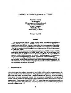
which is controlled dynamically has been shown in Figure 2 and the changes for the fuzzy control of the population size of the genetic algorithm have been shown in Figure 3.

(2)

j = Generation number, Pj = Population size in generation j, A1: The fitness value of the worst element (ξ) over the average fitness of all elements. A2 j = ζ j − ζ

(3)

j −1

j = Generation number, A2: The variance of the fitness value of the best element in two consecutive generations. The design of the fuzzy inference engine was to some extent inspired by [17]. These coefficients are multiplied by the former value of the population size and the probability of mutation rate and generate new values to be applied in the genetic algorithms. The fuzzy knowledge base used to regulate the coefficient applied to the probability of mutation in each generation consists of 16 rules with three inputs. The fuzzy knowledge base controlling the coefficient applied to the population size in each iteration consists of 17 rules with three inputs. the fuzzy rules used (FAM) are clearly shown in table 2.in order to design the fuzzy membership functions, triangular functions named Small (1), Medium(2), and Big(3) with [0 0 1.5], [0 1.5 3], and [1.5 3 3] coordinates were used.

A0 1

A1 1

A2 3

O 3

1

2

1

3

1

2

1

1

1

2

3

3

1

3

1

1

1

3

3

2

2

1

1

1

2

1

2

2

2

1

3

1

2

2

1

1

2

2

2

2

2

2

3

3

3

1

1

2

3

1

3

1

3

2

1

3

3

2

2

3

3

2

3

3

A0 1 1 1 1 1 2 2 2 2 2 2 2 3 3 3 3

A1 1 1 2 2 3 1 1 1 2 3 3 3 1 1 2 3

A2 1 3 2 3 1 1 2 3 1 1 2 3 1 3 3 3

O 1 2 2 3 2 2 3 2 2 3 2 2 1 3 3 1

)a(

)b( Table 2. a) FAM for Mutation Probability dynamic control. b) Population Size control for different generations Mutation 0.09 0.08

fn ( y ) dy

∫

µ fn ( y )dy

0.07

; fn ∈ [ A0 , A1 , A2 ]

(4)

V

Mamdani inference engine which is the most commonly seen fuzzy methodology along with the Center of Gravity defuzzifier (equation 4) was employed in the inference engine structure.

0.06 0.05 R a te

CoG fn =

∫ y.µ

V

0.04 0.03 0.02 0.01

After algorithm execution, the results show that although in the earlier generations of the genetic algorithm , the values of the probability of mutation and the size of the population that are controlled dynamically, had significant changes but after few generations and with adaptation to the problem nature, changes decrease and finally reach stability and don't change after then. Variance in the mutation probability

0 1 13 25 37 49 61 73 85 97 109 121 133 145 157 169 181 193 205 217 229 241 253 265 277 289 Generation

Dejong Fuzzy F#1

non fuzzy

Dejong Fuzzy F#2

Dejong Fuzzy F#3

Figure 2. Variance in Mutation Probability

Figure 5. Results for the second Dejong function (Generations axis has been divided by 100)

Population 160 140 120

Size

100 80 60 40 20 0 1

19

37

55

73

Dejong Fuzzy F#1 Dejong Fuzzy F#2

91 109 127 145 163 181 199 217 235 253 271 289 Generation non fuzzy

Dejong Fuzzy F#3

Figure 3. Population size change due to fuzzy control The results obtained from the evaluation of Dejong functions using the fuzzy parallel algorithm are shown in figures 4 to 6 respectively where the first 100, 40, 50 iterations in each diagram have been eliminated for visibility purposes. The results show an impressively quick convergence of the fuzzy parallel genetic algorithm. The algorithm will cause lower computation time because of its speed in reaching the global solution resulting in much lower resource (computational and communicational) consumption.

Experiments show that in the first Dejong function, our proposed algorithm reaches the global solution in the 100th generation while the other simple algorithms reach the global solution in the 150th generation, which shows a difference of 50 generations in reaching the global solution. The two other algorithms also with a difference of 40 and 20 generations show great performance, higher speed and a positive effect. The results obtained from the performed experiments on the proposed model show an optimized performance in the execution time (generation to reach the optimal solution). For genetic algorithm with a restricted generation, the proposed model by reaching the global solution quicker, can avoid premature convergence and prevent non optimal solutions due to insufficient generations.

Dejong 3rd Function

0.00E+00 Fuzzy non fuzzy

-5.00E+00 -1.00E+01 -1.50E+01 -2.00E+01

Dejong 1st Function

-2.50E+01

27

Value

31

29

21

23

25

15

Fuzzy 19

13

17

7

9

11

1

5

3

- 3.00E+01 Generation/10 1.80E+00 1.60E+00 1.40E+00 1.20E+00 1.00E+00 8.00E-01 Fuzzy

6.00E-01

non fuzzy

4.00E-01 2.00E-01 0.00E+00 1 2 3 4

5 6 7

8 9 10 11 12 13 14 15 16 17 18 19 20 21 22 23 24 Generation/10 25 26 27 28 29 30 31

Fuzzy

Figure 6. Third Dejong function results based on the proposed model (Generations axis has been divided by 100)

Value

5. Conclusion and Future Work Figure 4. First Dejong function results (Generations axis has been divided by 100) Dejong 2nd Function

3.00E-02

2.50E-02

2.00E-02

1.50E-02 Fuzzy non fuzzy

1.00E-02

5.00E-03

0.00E+00 1 2 3 4 5 6 7 8 9 10 11 12 13 14 15 16 17 18 19 20 21 22 23 24 Generation/10 25 26 27 28 29 30 31

Fuzzy

Value

The importance of the fuzzy parallel algorithm is well shown in the experiments by reaching the optimal solution and decreasing the amount of generations by lowering execution time. Significant decrease in execution time and generations to acquire the optimal solution promise a suitable reference model to solve complicated and time consuming problems using the fuzzy parallel genetic algorithms. For this reason applying dynamic control to crossover probability which hadn’t been studied in this experiment may have positive effects in reaching the optimal solution. On the other hand using fuzzy stop criteria can avoid useless algorithm execution, prevent useless system resource occupation and optimize processor usage.

6. References [1] Buck T, 1994, Selective pressure in evolutionary algorithms: a characterization of selection mechanism, proceeding of the first IEEE international Conference on Evolutionary Computing.

[14] Lin T., Lotfi A. Zadeh, Special issue on granular computing and data mining, 2004, Int. J. Intell. Syst. 19(7): 565-566. [15] Perfilieva I., Fuzzy function as an approximate solution to a system of fuzzy relation equations, 2004, Fuzzy Sets and Systems 147(3): 363-383.

[2] Dejong K., 1975, an analysis of the behavior of a class of genetic adaptive systems. PhD thesis, University of Michigan.

[16] Randy L., Haupt S., Practical Genetic Algorithms, 2003, Wiley-IEEE Publication.

[3] Goldberg D. E., Deb K., Thierens D., 1993, Toward a better understanding of mixing in genetic algorithms. Journal of the Society of Instrument and Control Engineers, vol. 32.

[17] Herrera F., and Lozano M., Fuzzy genetic algorithms: issues and models, , 1999, Dept. of Science and A. I., University of Granada, Technical Report No. 18071, Granada, Spain.

[4] Goldberg D. E., 1994. Genetic and evolutionary algorithms come of age. Communications of the ACM, vol. 37.

.

[5] Grosso P. B., 1985, Computer simulations of genetic adaptation: Parallel subcomponent interaction in a multilocus model. Doctoral dissertation, The University of Michigan [6] Harik G., Cantu-paz E., Goldberg D. E., Miller B. L., 1997, the gambler’s ruin problem, genetic algorithms, and the sizing of populations. In Proceedings of 1997 IEEE International Conference on Evolutionary Computation. [7] Jaja J., 1992.An Introduction to parallel Algorithms, Addison-Wesley [8] Herrera M., Lozano J., Verdagay L., 1995, Tuning fuzzy logic controllers by genetic algorithms. International Journal of Approximate reasoning. [9] Lin S. C., Punch W., Goodman E., 1994, Coarse-Grain Parallel Genetic Algorithms: Categorization and New Approach. In Sixth IEEE Symposium on Parallel and Distributed Processing. [10] Pwttey C. B., Leuze M. R., Grefenstette J., 1987, a parallel genetic algorithm. In Grefenstette J. J., Ed., Proceedings of the Second International Conference on Genetic Algorithms. [11] Lotfi A. Zadeh, Fuzzy algorithms, 1968, Information and Control, 12(2):94-102. [12] Sung-Kwun H., Pedrycz W., and Park B., Selforganizing neurofuzzy networks based on evolutionary fuzzy granulation, 2003, IEEE Transactions on Systems, Man, and Cybernetics, Part a 33(2): 271-277. [13] Rutkowski L., Siekmann H., Tadeusiewicz R., Lotfi A. Zadeh, Artificial Intelligence and Soft Computing, 2004, ICAISC 2004, 7th International Conference, Zakopane, Poland, June 7-11, Proceedings Springer.