s b k,n . Note that, although Ws transforms the 2-D space-time data into 2M time-domain ...... [4] Chia-Chang Hu, Irving S. Reed, and Xiaoli Yu, âBlind low-.
Delay and DOA Estimation for Chip-Asynchronous DS-CDMA Systems Using Reduced Rank Space-time Processing Chiao-Yao Chuang, Xiaoli Yu and C.-C. Jay Kuo Department of Electrical Engineering and Integrated Media Systems Center University of Southern California, Los Angeles, USA Abstract— A reduced-rank space-time processing algorithm is proposed in this work to estimate the time-delay and the direction-of-arrival (DOA) in short-code chip-asynchronous DS-CDMA systems. Most algorithms proposed before demand the inversion of the correlation matrix of received signals, which has a high computational cost. Here, we attempt to reduce the complexity by decomposing the correlation matrix inversion step into the cascade of multiple stages, where each stage outputs a scalar value that is obtained without an explicit matrix inversion operation. Furthermore, it is proved that the interference signals can be suppressed effectively using a small number of stages, and the performance is not much improved by applying more stages. Computer simulations are conducted to compare the performance of the reduced rank and the full rank approaches.
operation. Also, it is proved that the interference signals can be suppressed effectively with a small number of stages while the performance is not much improved by applying more stages. The rest of this paper is organized as follows. The signal and channel models are described in Sec. II. The preprocessing step using the beamforming filterbank is detailed in Sec. III. The time delay and the DOA estimation procedures, and the corresponding reduced rank decomposition scheme in the flat fading scenario are presented in Sec. IV. Simulation results are shown in Sec. V. Finally, concluding remarks are given in Sec. VI. II. Signal and Channel Models
I. Introduction Joint delay and DOA estimation algorithms using linear antenna arrays in DS-CDMA systems have been extensively studied recently. In [1], [2] and [3], the received space-time signal is stacked up into a long vector, and the maximum likelihood estimation is performed based on the training sequence. Let L and M be the processing gain of the short code and the number of antennas, respectively. The advantage of this approach is that the receiver at the base station is able to accommodate the number of total signals more than L, since the correlation matrix of this long vector has a dimension of M L × M L. If the correlation matrix is unknown and must be estimated from the received data, M L data points are required to avoid rank deficiency. Then, the stationary assumption has to hold for a longer while, making it challenging to achieve in practice. Hu et al. [4] employed the multistage Wiener filter to reduce the complexity, where the stacking up method was still adopted and a training sequence was sent to estimate the spatial information since the impinging desired signals have unknown DOAs. A full rank space-time processing algorithm was developed for the flat fading channel in [5] and for the frequency selective fading channel in [6]. In these two papers, we solved the major shortcoming of the stacking-up method, namely, the requirement of a larger data support (or the longer synchronization time) to provide better estimation of the correlation matrix of the space-time signal. Simply speaking, we used a beamforming filterbank to transform received two-dimensional space-time signals into several one-dimensional time-domain sequences. However, the inverse of a correlation matrix of dimension L × L is still required in [5] and [6] since both of them are based on a full-rank approach. In this work, we show that the complexity can be further reduced by decomposing the inversion of a full rank matrix into multiple stages, where each stage outputs a scalar value that is obtained without an explicit matrix inversion IEEE Communications Society / WCNC 2005
255
Consider a BPSK DS-CDMA system with K independent users. User k, k = 1, 2, .., K, is assigned a distinct short PN L−1 with L chips, and transmits the signal code {ck (l)}|l=0 +∞ L−1 � �√ Edk (j)ck (l)ψ(t − lTc − jT ), uk (t) = j=−∞ l=0
where Tc and T denote the chip and the symbol periods, respectively, ψ(t) is the rectangular pulse with the period √ �T 0 ∼ Tc and E 0 c ψ(t)dt = 1, and dk (j) represents the BPSK symbol with index j from user k. Finally, grouping L−1 into a vector, then normalizing to 1 gives the {ck (l)}|l=0 representation sk = [ck (0), .., ck (L − 1)]T and �sk � = 1, for each k. The wireless channel is approximated by the following tapped delay line model Nk � hk (τ ; t) = Ak,n (t)δ(τ − τk,n ) n=1
for user k. The time delay τk,n can be written as (γk,n + �k,n )Tc , where γk,n is a positive integer and �k,n , the fractional component of delay, has the range 0 ≤ �k,n < 1. It is also assumed that the largest path delay difference is less than one symbol period, namely | maxn {τk,n } − Nk minn {τk,n }| < T for all users. {Ak,n (t)}|K k=1 |n=1 is a set of statistically independent complex zero-mean wide-sense stationary Gaussian random processes. Let us use y c,k,n (t) = bk,n Ak,n (t)uk (t − τk,n ), where bk,n , normalized to be of the unity norm, is an M -dimensional vector denoting the spatial signature of the n-th path of user k at an M -element antenna array. Also, as a result of the linear antenna array, we have −1 bk,n = M 2 [1, e−iπ sin θk,n , · · · , e−iπ(M −1) sin θk,n ]T . (1) Then, the received signal at the antenna array becomes Nk K � � y c (t) = y c,k,n (t) + n(t), k=1 n=1
where the subscript c simply denotes the signal in the continuous-time format. 0-7803-8966-2/05/$20.00 © 2005 IEEE
III. Pre-processing with Multibeam Filterbank The received signal y c (t) is passed through the chipmatched filter employed at each array element and then sampled at the chip rate. Let index ti stand for the sampling at each chip-matched filter output integrating from ti Tc to (ti + 1)Tc . Then, the discrete-time vector, with a dimension of M × 1 after sampling, can be written as � (t +1)Tc y d (ti ) = ti Tic y c (t)dt. Grouping together these vectors corresponding to distinct indexes yields Yd = [y d (0), y d (1), y d (2), y d (3), · · · , y d (ti ), ...]. Simply speaking, Yd represents the 2-D space-time discretetime data after sampling. The further processing on Yd is essential before conducting the estimate of parameters. For instance, the methods in [1], [2] and [3] stack up the discrete 2-D space-time data into a long vector of dimension M L×1. A reduced rank operation, called space-nonadaptive time-adaptive processing, uses a fixed spatial DFT filterbank to transform Yd into a time-domain vector, on which adaptive processing is performed. The design of the spatial i2π DFT filterbank is not unique. Let zM = e− M . The spatial DFT filterbank is in general given by FM = M
−1 2
which indicates the appearance of sk , the assigned PN code Nk for user k. As shown above, {ak,n }|K k=1 |n=1 is the set of discrete-time slow fading parameters, which are unknown constants during the synchronization process. Without the loss of generality, we confine the search of the desired signal in the sliding windows with ∆ = 0, 1, .., L − 1. IV. Blind Time Delay and DOA Estimation A. Full Rank Estimation Scheme in Flat Fading
M −1 Vandermonde(1, zM , ..., zM ),
M −1 where Vandermonde(1, zM , ..., zM ) represents a VanderM −1 . As shown monde matrix constructed by 1, zM , ..., zM above, the m-th column in FM , m = 1, 2, .., M , can be treated as a beamforming filter, with a unique steering direction in the space domain. Since the linear array covers the range −90◦ ≤ θ ≤ 90◦ in the azimuth angle, corresponding to −1 ≤ sin(θ) ≤ 1, thus FM collects these beam, if 2(m−1) ≤ M , forming filters steering at sin(θ) = 2(m−1) M ) and 2(m−1−M , if 2(m − 1) > M . M We can alter the steering direction of each beamforming filter in FM and maintain the orthogonality between them by simply shifting an equal amount of angle for each. Let M −1 2 , · · · , z2M ). ΩM = diag(1, z2M , z2M Then, ΩM FM is also a spatial DFT filterbank, steering at 2(m−M )−1 , if 2(m − sin(θ) = 2m−1 M , if 2m − 1 ≤ M and M M) − 1 > M. We can combine FM and ΩM FM to form a nonadaptive multibeam filterbank with 2M beamforming filters, denoted by Ws . For convenience, Ws is constructed by interleaving the columns of FM and ΩM FM . As a result, Ws is an M × 2M matrix. Let T X = WH s Y d ≡ [ x1 , ..., x2M ] represent 2M time-domain sequences as the beamforming filterbank output. As indicated above, X and Yd share the same time index. A sliding window is applied to X to collect L consecutive samples from each row, where the window slides one chip at one time. Mathematically, we have T T x1 [0 : L − 1] x1 [∆ : L + ∆ − 1] .. .. SW(0)= , ..SW(∆)= , . .
xT2M [0 : L − 1] xT2M [∆ : L + ∆ − 1] where SW(0) collects the samples from ti =0 to L − 1, etc. A complex response vector of dimension 2M × 1, reflecting the DOA of the n-th path of user k on the beamforming IEEE Communications Society / WCNC 2005
filterbank, can be written as Γk,n = WH s bk,n . Note that, although Ws transforms the 2-D space-time data into 2M time-domain sequences, the spatial information for DOA still resides in Γk,n . Let T and T be acyclic right- and left-shift operators, respectively. It is assumed that the synchronization process starts at ∆ = 0. As the sliding window moves to ∆ = γk,n , the signal corresponding to the n-th path of user k is given by �
T SW(γk,n ) = ak,n Γk,n �k,n dk (j) T sk + T
� + (1 − �k,n )dk (j)sTk , (2) �k,n dk (j − 1) T L−1 sk
256
In this subsection, we review the full rank algorithm for delay and DOA estimation as described in [5]. Let user 1 be the desired user with code s1 and sliding window ∆ = γ1,1 be the in-lock window. Some notations are defined below for later use: sr =T s1 =[0, s1 [0 :L − 2]T ]T , S1 = [s1 , sr ] and ι = [1 − �1,1 , �1,1 ]T . The method proposed in [5] adopts a time-domain datadependent linear filter for each row in SW(∆), denoted by (∆) wt,m . The filter is derived by solving the following constrained optimization problem, (∆)H
(∆)H
(∆)
(∆) T ψm = min wt,m R(∆) m w t,m , s.t. w t,m C = g .
By applying C = S1 and g = [1, 1] , we get −1 � −1 T (∆) = [ 1, 1 ] ST1 R(∆) S1 [ 1, 1 ] , ψm m
(3)
T
(4)
where R(∆) m denotes the correlation matrix of the m-th row ( i.e. the m-th beamforming filter output) in the sliding window ∆. This operation aims at protecting the subspace spanned by s1 and sr by imposing two constraints while all other vectors are suppressed. If the desired signal is present in the system, the coarse synchronization stage estimates the parameter γ1,1 via (∆) (� γ1,1 , M1 ) = arg max max ψm , ∆
M2 = arg max
m\M1
m
(� γ1,1 ) ψm ,
0 ≤ ∆ ≤ L−1, 1 ≤ m ≤ 2M,
which also gives M1 and M2 , denoting the beamforming filters with the largest and the second largest outputs in the estimated in-lock window γ �1,1 . The estimate of |a1,1 Γ1,1 [m]|2 can be realized by imposing Woodbury’s inverse formula to obtain (� γ1,1 )−1 T (� γ1,1 ) =|a1,1 Γ1,1 [m]|2 +[ 1, 1 ] (ST1 RN ,m S1 )−1 [ 1, 1 ] , (5) ψm (� γ1,1 ) if γ �1,1 = γ1,1 . The matrix RN ,m stands for the MAI plus noise covariance matrix in the estimated in-lock window.
0-7803-8966-2/05/$20.00 © 2005 IEEE
The second term at the right hand side in (5) is the noise power after suppression. In the out-of-lock windows, the corresponding outputs are equal to the noise power after suppression. The proposed DOA estimation algorithm first identifies the section from which the desired signal may come, and then estimates θ1,1 herein. To identify the proper section, we employ the property that each section has its correspondence with a unique pair of the beamforming filter outputs producing the two largest responses, and then a fine search algorithm is performed in the identified section. By collecting the two largest soft values from the estimated in-lock window, normalizing to form an information vector, then constructing its orthogonal projection, we get � �T γ1,1 ) �(� γ1,1 ) � = ψ�(� �ψ � 2. � T /�ψ� ψ , P� =ψ (6) ψ M1 , ψM2 A new steering vector with two elements is developed for the fine-scale search, which is written as � � � �M −1 −i·vπ sin(θ) �2 1+ e � � 1 v=1 �2 , bs (sin(θ)) = 2 � � � M −1 −i·vπ(sin(θ)− 1 ) � M M � �1+ v=1 e 1 . Then, the fine-scale with sin(θ) ranging from 0 ∼ 2M search algorithm is conducted as �bs (sin(θ))�2 � = arg max sin(θ) , (7) sin(θ) bs (sin(θ))T (I2×2 − P )bs (sin(θ)) � ψ
� stand for the where I2×2 is a 2 × 2 identity matrix. Let Ξ identified section. The azimuth angle θ1,1 of the desired user can be derived through the transformation � (� Ξ−2M −1) 180 � � odd ) ,Ξ � π · asin(sin(θ) + 2M θ1,1 = (8) � ( Ξ −2M −1) 180 1 � + � even · asin( − sin(θ) ) ,Ξ π
2M
2M
j=1
where {cj } and {β j }, 1 ≤ j ≤ nI , represent the coefficient vectors of projecting the j-th interfering signal on −1 S1 (ST1 S1 ) 2 and B1 , respectively. Then, {cj } and {β j } are 2-dimensional and (L−2)-dimensional vectors, respectively. The energy output from the matched filter can be expressed as nI � T (γ1,1 ) [1, 1] GT1 Rm G1 [ 1, 1 ] =|a1,1 Γ1,1 [m]|2 + σj2 j=1 2
B. Reduced Rank Estimation Scheme The inverse of correlation matrix R(∆) m of dimension L×L is required in (4), which demands a complexity of O(L2 ) if a fast algorithm is applied. It is possible to reduce the computational complexity by deriving an equivalent procedure that carries out the matrix inversion in a smaller dimension. Let H1 be an L×L nonsingular matrix with the following property � T� � � I2×2 G1 = H 1 S1 = S 1 0(L−2)×2 , BT1 where G1 is equal to S1 (ST1 S1 )−1 , B1 , an L × (L − 2) matrix, is orthogonal to S1 , I2×2 is a 2 × 2 identity matrix, and 0(L−2)×2 simply represents an (L − 2) × 2 zero matrix. By applying the nonsingular property H−1 1 H1 = IL×L and inserting into (4), we have � −1 −1 T T [ 1, 1 ] ST1 R(∆) S [ 1, 1 ] = [ 1, 1 ] GT1 R(∆) 1 m G1 [ 1, 1 ] m T (∆) −1 T (∆) − [ 1, 1 ] GT1 R(∆) B1 Rm G1 [ 1, 1 ] . (9) m B1 (B1 Rm B1 ) It is evident that the first term above does not require matrix inversion. The inverse of BT1 R(∆) m B1 in the second term is operated in a subspace of dimension (L − 2) × (L − 2), which is smaller than that of R(∆) m . The physical meaning in (9) can be explained as follows. The received signal is projected onto both the filterbank S1 , T
IEEE Communications Society / WCNC 2005
which is the subspace of the desired signal, and the filterbank B1 , which is the subspace orthogonal to S1 . Simply speaking, the projection on S1 is the matched filter operation. The filterbank S1 is unable to block any of the interfering signals that are not orthogonal to it. Then, the signals that are not orthogonal to S1 also pass through filterbank B1 while the desired signal is blocked at this stage. The energy of these interfering signals through S1 can be estimated by observing the energy captured in B1 as well as the cross-correlation of the energies through S1 and B1 . It becomes evident if we express the white noise and the −1 MAI in the form of S1 (ST1 S1 ) 2 and B1 , both constructing the basis of vector space RL . The MAI, treated as structural noise, can be written as the linear combination of the above-defined basis. The white noise, which has a non-structural nature, has an equal amount of power on each basis vector. Let the number of interfering signals be nI . The correlation matrix in the in-lock window can be rewritten as (γ1,1 ) Rm =|a1,1 Γ1,1 [m]|2 S1 ιιT ST1 +σ 2 S1 (ST1 S1 )−1 ST1 +σ 2 B1 BT1 nI � −1 −1 + (S1 (ST1 S1 ) 2 cj +B1 β j )(S1 (ST1 S1 ) 2 cj +B1 β j )T , (10)
257
1] (ST1 S1 )−1
T
+σ [1, [ 1, 1 ] , (11) where a simplified notation is used to represent the energy from the interfering signal. We have σj2 = [ 1, 1 ] (ST1 S1 )
−1 2
cj cTj (ST1 S1 )
−1 2
T
[ 1, 1 ] .
The block filter generates the following output βT σ1 nI −1 � � .1 � 2 � T σ I+ .. . , · · · , β β . [ σ1 , · · · , σnI ] β β 1 nI . . j j j=1 σnI β Tn I
In above, the combined three middle terms can be treated as an orthogonal projection matrix in a underdetermined system with the perturbation term σ 2 I(L−2)×(L−2) . If σ 2 ≈ 0, the orthogonal projection matrix converges to an nI × nI identity matrix. Then, the block filter output becomes σ12 + .. + σn2 I , which completely cancels the interference energy from the matched filter output. Let us consider an example. If nI = 1, the orthogonal projection matrix is � −1 β T1 σ 2 I(L−2)×(L−2) + β 1 β T1 β 1 = β T1 β 1 (β T1 β 1 + σ 2 )−1 , which converges to 1 as σ ≈ 0. The system is of full rank when nI = L − 2. The property that the orthogonal projection matrix converges to an identity matrix with negligible 0-7803-8966-2/05/$20.00 © 2005 IEEE
σ 2 is maintained as long as nI ≤ L − 2. However, this property does not hold when the system becomes overdetermined, i.e. nI > L − 2, even with negligible σ 2 . This is due to the fact that the projection on a subspace of a dimension which is smaller than that of vector space RnI . Some concluding remarks can be drawn based on results presented above. 1. With negligible σ 2 , the interference effect can be completely removed if nI ≤ L − 2. 2. If nI ≤ L − 2, the increase of σ 2 leads to the underestimate of the interference. Then, the interference cannot be removed completely. 3. If nI > L − 2, the interference cannot be removed completely even with negligible σ 2 . Then, the best that the system can do is to restrict the number of the interference signals to be no more than L − 2.
D. Analysis of Truncated Multistage Decomposition
C. Matrix Inversion via Multistage Decomposition
In the following derivation, we assume that the condition nI ≤ L − 2 holds. Let a2 [j] be the j-th element and 1 ≤ j ≤ L − 2. A simple way to construct B2 is to define a2 [1] a2 [1] · · · a2 [1] .. .. −a2 [1]2 . . a2 [2] � L−4 2 , (15) − a [j] B2 = 2 j=1 a [L − 3] 0 �2 a2 [L−3] L−3 .. − a2 [j]2 j=1 0 · · · . a2 [L−2] � � 1 1 � � � � Λ�B2 � =diag � �L−2 B2 [i,1]2 � , · · · , � �L−2 B2 [i,L−3]2 � .
The second term in (9) can be further decomposed using the same methodology as applied to the decomposition of (4). Let us define BT R(∆) G1 [ 1, 1 ] a2 = � 1 m T (∆) �2 , R2 = BT1 R(∆) m B1 , �[1, 1]G1 Rm B1 � and H2 , a nonsingular matrix of dimension of (L−2)×(L− 2), has the following form T
T
H2 = [ a2 , B2 ] . As shown above, a2 is an (L−2)×1 vector, and B2 , a matrix orthogonal to a2 , has a dimension of (L − 2) × (L − 3). By applying H−1 2 H2 = I(L−2)×(L−2) to the second term in (9) , the equivalent expression is derived as (12) (aT2 R2 a2 − aT2 R2 B2 (BT2 R2 B2 )−1 BT2 R2 a2 )−1 . The second term in the denominator of (12) can also be decomposed in the same manner. Let us define BT R2 a2 T T a3 = � T2 � , R3 = B2 R2 B2 , and H3 = [ a3 , B3 ] , �B2 R2 a2 �2 where a3 , B3 and H3 are of dimension (L − 3) × 1, (L − 3) × (L − 4) and (L − 3) × (L − 3), respectively. Then, we can rewrite (4) of the equivalent form as [ 1, 1 ] GT1 R(∆) m G1[ 1, 1 ] −
T
1
. − We see from above that the only matrix inversion needed is for BT3 R3 B3 , which has a dimension of (L − 4) × (L − 4). Likewise, the decomposition can be done repeatedly by defining aT2 R2 a2 −(aT3 R3 a3
aT3 R3 B3 (BT3 R3 B3 )−1 BT3 R3 a3 )−1
BT Ri ai T ai+1 = � Ti � , Ri+1 = Bi Ri Bi . �Bi Ri a �2 i Then, a multistage representation of (4) can be written as � � 1 1 T (∆) 1, 1 [ ] G1 Rm G1 1 − T . (13) 1 a2 R2 a2 − T a3 R3 a3 − T 1 a4 R4 a4 − ··· As shown above, ai Ri ai is the i-th stage operation, where i starts from 2. The matched filter operation shown in the first term is defined as the first stage. IEEE Communications Society / WCNC 2005
258
It was shown in the last subsection that the full rank matrix inversion in (4) is equivalent to (13) without explicit matrix inversion. The computation can be further reduced if only a finite number of stages is needed to result in satisfactory performance. It is therefore interesting to study the relationship between the number of stages and the number of interference signals. If the interference signals can be suppressed within a finite number of stages, the performance of the reduced rank operation is comparable with that of the full rank operation. Let us follow the setup of the correlation matrix in (10), and start �nwith I nI � j=1 β j σj 2 , R =σ I + β j β Tj . (14) a2 = �nI 2 (L−2)×(L−2) � j=1 β j σj �2 j=1
i=1
i=1
Note that if a2 [j] is equal to zero, the corresponding column having it at the denominator is replaced by [0T(j−1) , 1, 0T(L−2−j) ]T . Then, we have B2 = B2 Λ�B2 � . (16) Using the eigen-decomposition, R2 can be represented as � �� T � Λ + σ 2 InI ×nI 0nI ×(L−nI −2) Us R2 = [Us , Un ] s , 0(L−nI −2)×nI σ 2 I(L−nI −2)×(L−nI −2) UTn where Λs = diag[λ1 , · · · , λnI ], Us = [u1 , · · · , unI ], and Un = [unI +1 , · · · , uL−2 ], which are of dimensions nI × nI , (L − 2) × nI and (L − 2) × (L − nI − 2), respectively. Since the subspace spanned by {β 1 , · · · , β n } is equal to that by I eigenvectors {u1 , · · · , unI }, vector a2 can be expressed as a2 = κ1 u1 + · · · + κnI unI ≡ Us κ, where κ = [κ1 , · · · , κnI ]T is the coefficient vector. Similarly, B2 = Us Cs + Un Cn , where Cs and Cn are nI ×(L−3) and (L−nI −2)×(L−3) coefficient matrices, respectively. Accordingly, the following conditions must hold between κ, Cs and Cn : (1) CsT κ = 0, (2) CsT Cs +CnT Cn = I(L−3)×(L−3) , (3) Rank(Cs ) = nI −1 and (4) Cs CnT = 0nI ×(L−nI −2) . Then, we have CsT Λs κ . (17) �CsT Λs κ�2 The above result indicates that the signal subspace contained by R3 has a rank of nI − 1, which is one rank less than that of R2 . The vector a3 can be expressed as a linear combination of nI − 1 eigenvectors belonging to the signal subspace. The block matrix B3 can be derived by following the same procedure as we construct B2 with (15) and (16). R3 = CsT Λs Cs + σ 2 I(L−3)×(L−3) , a3 =
0-7803-8966-2/05/$20.00 © 2005 IEEE
Simply speaking, the dimension of Ri is (L − i) × (L − i) with a rank equal to L − i. The signal and noise subspaces in Ri have ranks nI + 2 − i and L − nI − 2, respectively. When i = nI + 1, B(nI +1) is completely described by the noise subspace, and the signal subspace in R(nI +1) is only of rank one. Thus, we have BT(nI +1) R(nI +1) a(nI +1) = 0. This means that the effect of nI + 1 cascaded stages is equivalent to the full rank operation in suppressing nI interference signals, making further decomposition unnecessary. To conclude, when nI ≤ L − 2, we have the following equality: −1 � −1 T T [ 1, 1 ] ST1 R(∆) S [ 1, 1 ] = [ 1, 1 ] GT1 R(∆) 1 m G1 [ 1, 1 ] m 1 aT2 R2 a2
−
aT3 R3 a3 − ... −
1
.
(18)
aT(nI +1) R(nI +1) a(nI +1)
−1
10
E. Improvement of DOA Estimation So far, the analysis is based on the correlation matrix derived by the ensemble average. With the substitution of � (∆) in (3), the average output R(∆) by the sample matrix R m
m
energy in (4) is of the same form with R(∆) replaced by m (∆) � . Interestingly, the average output energy in the inR m lock window as shown in (5) is not, as expected, obtained � (γ1,1 ) for R(γ1,1 ) . Instead, it is of by simply substituting R N ,m
N ,m
the following form −L+2 �√ �2 Ns� � (γ1,1 ) � (γ ) (γ1,1 ) = � ρm a1,1 Γ1,1 [m] + ς1,m + |ςj,m1,1 |2 , (19) ψ�m � j=2
where ρm is a Beta random variable, expressed as and Beta(Ns − L + 2, L − 2), with E[ρm ] = (Ns −L+2) Ns (γ
)
Ns −L+2 var(ρm ) = (NsN−L+2)(L−2) , and {ςj,m1,1 }|j=1 is a set of 2 s (Ns +1) i.i.d. complex Gaussian random variables, each of which obeys the following distribution � � � 1 (γ ) (γ1,1 )−1 ςj,m1,1 ∼ CN 0, Ns−1 [ 1, 1 ] (ST1 RN ,m S1 )−1 1 . (20)
Note that ρm is only a function of the number of data support, Ns , and the short code length L, regardless of the noise structure and the corresponding power. The physical meaning of the form of ρm can be explained as follows. Even if the desired user is assumed to be uncorrelated with other interfering users and noise, the correlation still exists when a finite number of data support is collected to construct the correlation matrix. Then, the sample matrix, the correlation matrix derived using the time average of finite data support, is of the following form in the in-lock window � (γ1,1 ) =(a1,1 Γ [m]S1 ι+� � m, R µm )(a1,1 Γ1,1 [m]S1 ι+� µm )H +Σ m 1,1 with v(1) µ �m = √ , Ns
0
10
1
Ns � �m = 1 Σ v(j)v(j)H . Ns j=2
−2
10
−3
10
theory simulation −4
10
0
0.2
0.4 0.6 0.8 Value of Beta random variable
1
Fig. 1. The curves from the left to right: Ns = 40, 50, 60, 70, 80, 90, 100, 120, 150 and 200, and L is fixed with 31. Each curve is plotted with 104 trials.
The proposed DOA estimation scheme that utilizes two largest beamforming filter outputs introduces the error due to the existence of ρm , even with negligible MAI and AWGN power. To illustrate this point, let us ignore the cross-product term in (19). Then we have the following information vector � � � �Ns −L+2 (γ1,1 ) 2 � 2 2 |ςj,M1 | ρ |a | |Γ [M ]| M 1,1 1 1 1,1 �= ψ + �j=1 Ns −L+2 (γ1,1 ) 2 . (21) ρM2 |a1,1 |2 |Γ1,1 [M2 ]|2 |ςj,M2 | j=1 Despite that two Beta random variables ρM1 and ρM2 , as shown above, have the same control parameters for the distribution, they may not be equal to each other. As a result, the vector [|Γ1,1 [M1 ]|2 , |Γ1,1 [M2 ]|2 ]T residing in the DOA information is perturbed. This behavior occurs with finite data support. Although the error variance can be reduced by increasing the length of data support, which however requires a longer synchronization time to mitigate the influence of the Beta random variables. The second vector at the right hand side of (21) is the noise power after suppression. Both the full rank and reduced rank operations, as shown in (4) and (18), respectively, attempt to reduce this term. Based on the ensemble average analysis, the reduced rank operation is equivalent to the full rank operation. Under the time average case, the effect of the Beta random variables is expected to be less severe for the reduced rank approach since it can suppress interference signals effectively with a smaller number of stages. Note that the desired signal could be suppressed in stages that are more than necessary. V. Simulation Results
s The random vectors in set {v(j)}|N j=1 , as shown above, are uncorrelated with one another. Each of them follows the distribution (γ1,1 ) v(j) ∼ CN (0L×1 , RN ,m ).
IEEE Communications Society / WCNC 2005
Log CDF
−
The additive vector µ �m perturbs the desired signal S1 ι, causing the mismatch with the outward steering matrix S1 in (4). Then, the suppression on the desired signal is conducted, which subsequently forces the power to be Betadistributed. Finally, in the limit case with Ns → +∞, (19) converges to (5). The derivation of (19) is not given here due to the space limit. To validate the Beta random variable in (19), we compare theoretical and experimental results in Fig. 1, where the cumulative density function (of the log scale) is plotted as a function of the Beta random variable parametrized by different values of Ns . We see a close match of the curves.
259
Simulation results are provided to demonstrate the performance of the proposed reduced rank delay and DOA estimation algorithm. We simulated a BPSK/CDMA system with the Gold code of length L = 31. A linear beamforming 0-7803-8966-2/05/$20.00 © 2005 IEEE
full rank 3 stages 6 stages 12 stages
9
8 7 6 5 4 3 2
1
0 40
60
80 100 120
150
The number of data support
(a)
200
10
full rank 3 stages 6 stages 12 stages
9
8
7
6 5
4
3
2 1 0 40
60
80 100 120
150
200
DOA root average squared error (degree)
10
DOA root average squared error (degree)
DOA root average squared error (degree)
The number of data support
(b)
10
full rank 3 stages 6 stages 12 stages
9 8 7 6 5
Correct coarse synchronization rate
Correct coarse synchronization rate
0.995
1
0.99
0.99
0.98
0.985 0.98
0.97
0.975
full rank 3 stages 6 stages 12 stages
0.97
0.965
0.96 31 40
60
80
100
full rank 3 stages 6 stages 12 stages
0.96
0.95
150
200
0.94 31 40
60
80
0.98
0.96
full rank 3 stages 6 stages 12 stages
0.92
0.9 31 40
60
80
100
150
200
(b)
150
The number of data support
200
Correct coarse synchronization rate
(a) 1
0.94
100
The number of data support
The number of data support
1
0.95 0.9 0.85
0.8
full rank 3 stages 6 stages 12 stages
0.75 0.7
0.65 31 40
60
(c)
80
100
150
200
The number of data support
(d)
Fig. 3. Coarse synchronization rate with (a) 5 users, (b) 8 users, (c) 11 users and (d) 18 users.
VI. Conclusion A reduced-rank delay and DOA estimation algorithm for the synchronization of short code DS-CDMA systems was developed in this work. The inversion of the full-rank correlation matrix can be replaced by a cascaded reduced-rank approach. When the received signal’s correlation matrix is estimated using finite data support, the desired signal is also suppressed by the full rank operation as a result of mismatch. However, the suppression on the desired signal can be mitigated by applying the multistage scheme as long as the number of stages is sufficient to suppress the interference. Our analysis was confirmed by simulation results, which showed that the multistage scheme is able to provide satisfactory performance with a short number of data support, which means that synchronization can be achieved more rapidly.
4
References
3
[1] Kun Wang and Hongya Ge, “Joint estimation of time delays and DOA’s for DS-CDMA system over multipath Rayleigh fading channels,” IEEE ICC, vol. 5, pp. 1436–1440, 2001. [2] A.A. D’Amico, U. Mengali, and M. Morelli, “Joint DOA and channel parameter estimation for code-division multiple-access systems,” IEEE ICC, 2003. [3] C. Sengupta, J. R. Cavallaro, and B. Aazhang, “On multipath channel estimation for CDMA systems using multiple sensors,” IEEE Trans. on Communications, vol. 49, pp. 543–553, Mar 2001. [4] Chia-Chang Hu, Irving S. Reed, and Xiaoli Yu, “Blind lowcomplexity code-timing acquisition for space-time asynchronous DS-CDMA signals,” IEEE GlobeComm, 2002. [5] C. Y. Chuang, X. Yu, and C. C. Jay Kuo, “ Space-time blind delay and DOA estimation in chip-asynchronous DS-CDMA systems,” IEEE GlobeComm, 2004, to appear. [6] C. Y. Chuang, X. Yu, and C. C. Jay Kuo, “ Blind delay and DOA estimation in correlated multipath DS-CDMA systems,” VTC Fall, 2004, to appear.
2
1
0 40
60
80 100 120
150
200
The number of data support
(c)
Fig. 2. The root mean square error of DOA as a function of the number of data support with (a) 5 users, (b) 8 users and (c) 11 users.
The correct coarse synchronization rate is plotted in Fig. 3 for difference user numbers. We see that, as the number of users increases, the reduced rank approach with a smaller number of stages performs poorly due to its poor capabilIEEE Communications Society / WCNC 2005
ity to suppress interference. Again, this demonstrates the importance of balancing the user and the stage numbers to improve the performance.
Correct coarse synchronization rate
array at the base station with two elements was employed. We fixed the number of stages to be 3, 6 and 12, and studied the performance with a different number of users. We considered three different cases with the number of users equal to 5, 8 and 11, respectively. The near-far ratios for all interfering users and the SNR value were set to 5dB and 10dB, respectively. Experimental curves were obtained with 4000 trials. The parameters γk,n (integer delay), �k,n (fractional delay) and θk,n (DOA) were randomly chosen between 0 ∼ L − 1, 0 ∼ 1 and −90◦ ∼ 90◦ , respectively, on each trial. Since our current work is primarily focused on the coarse synchronization and the DOA estimation, simulation results of fractional delay estimation are not provided. The number of data support, Ns , is proportional to the number of data bits allowed for synchronization. The correlation matrix R(∆) is constructed using the allowed m data support. It is required that Ns be larger than L to avoid the rank deficiency of the correlation matrix. Fig. 2, consisting of three subfigures for the case of 5, 8 and 11 users, respectively, showed the root average square error of DOA estimation conditioned on correct coarse synchronization. Each subfigure has 4 curves, denoting the full rank operation, the reduced rank operations with 3 stages, 6 stages and 12 stages, respectively. Fig. 2(a) was simulated at a light-loaded scenario with 5 users. We see that, with finite data support, a small number of stages is able to perform well as compared with the full rank operation. However, there is an error floor for the 3-stage scheme as the data support exceeds 100, which is caused by the limited suppression capability on the other 4 asynchronous interfering users. Fig. 2(b) depicts the performance curves with 8 users, where the 3-stage scheme has a higher error floor. Fig. 2(c) shows the curves with 11 users, where the 3-stage and 6-stage schemes have limited capability to suppress the interference, leading to unacceptable error floors. From these simulation results, we conclude that the protection of the desired signal and the suppression of the interference are equally important. Then, the number of stages to be adopted should be adaptive with respect to the number of interfering signals (i.e. other users).
260
0-7803-8966-2/05/$20.00 © 2005 IEEE