Delay Bounds In a Network With Aggregate ... - Semantic Scholar

A. Charny

Delay Bounds In a Network with Aggregate Scheduling. Draft Version 4. 2/29/00

Delay Bounds In a Network With Aggregate Scheduling1 Anna Charny [email protected]

Abstract

ra f

t

A large number of products implementing aggregate buffering and scheduling mechanisms have been developed and deployed, and still more are under development. With the rapid increase in the demand for reliable end-to-end QoS solutions, it becomes increasingly important to understand the implications of aggregate scheduling on the resulting QoS capabilities. This document studies the bounds on the worst case delay in a network implementing aggregate scheduling. A lower bound on the worst case delay is derived. It is shown that in a general network configuration the delays achieved with aggregate scheduling are very sensitive to utilization and can in general be quite high. It is also shown that for a class of network configurations described in the paper it is possible to give an upper bound that provides reasonable worst case delay guarantees for reasonable utilization numbers. These bounds are a function of network utilization, maximum hop count of any flow, and the shaping parameters at the network ingress. It is also argued that for a general network configuration and utilization numbers which are independent on the maximum hop count, an upper bound on delay, if it exists, must be a function of the number of nodes and/or the number of flows in the network.

1.0 Introduction 1.1 Motivation

In the last decade, the problem of providing end-to-end QoS in the Integrated Services networks has received a lot of attention. One of the major challenges in providing hard end-to-end QoS guarantees is the problem of scalability. Traditional approaches to providing hard end-to-end QoS guarantees, which involve per flow signalling, buffering and scheduling, are difficult, if not impossible, to implement in very high-speed core equipment. As a result, methods based on traffic aggregation have recently become widespread. A notable example of methods based on aggregation has been developed in the Differential Services Working

D

group of IETF. In particular, [4] defines Expedited Forwarding per Hop Behavior (EF PHB), the underlying principle of which is to ensure that at each hop the aggregate of traffic requiring EF PHB treatment receives service rate exceeding the total bandwidth requirements of all flows in the aggregate at this hop. Recently, a lot of practical implementations of EF BHB have emerged where all EF traffic is shaped and policed at the backbone ingress, while in the core equipment all EF traffic shares a single priority FIFO or single high-weight queue in a Class-Based Fair Queuing scheduler. Since these implementations offer a very high degree of scalability at comparatively low price, they are naturally very attractive.

Sufficient bandwidth must be available on any link in the network to accommodate bandwidth demands of all individual flows requiring end-to-end QoS. One way of ensuring such bandwidth availability is by generously over provisioning the network capacity. Such over provisioning requires adequate methods for measuring and predicting traffic demands. While a lot of work is being done in this area, there remains a substantial concern that the absence of explicit bandwidth reservations may undermine the ability of the network to provide hard QoS guarantees. As a result,

1. This document is draft that is a substantially revised from its previous version.

Copyright © 1998 Cisco Systems, Inc. All Rights Reserved

Page 1 of 31

A. Charny


approaches based on explicit aggregate bandwidth reservations using RSVP aggregation are being proposed [1]. The use of RSVP aggregation allows the uncertainty in bandwidth availability to be overcome in a scalable manner. As a result, methods based on RSVP aggregation can provide hard end-to-end bandwidth guarantees to individual flows sharing the traffic aggregate with a particular aggregate RSVP reservation. However, regardless of whether bandwidth availability is ensured by over provisioning, or by explicit bandwidth reservations, there remains a problem of whether it is possible to provide not only bandwidth guarantees but also endto-end latency and jitter guarantees for traffic requiring such guarantees, in the case when only aggregate scheduling is implemented in the core. An important example of traffic requiring very stringent delay guarantees is voice. A popular approach to supporting voice traffic is to use EF PHB and serve it at a high priority. The underlying intuition is that as long as the load of voice traffic is substantially2smaller than the service rate of the voice queue, there will be no (or very little) queueing delay and hence very little latency and jitter. However, little work has been done in quantifying just exactly how much voice traffic can actually be supported without violating stringent end-to-end delay

t

budget that voice traffic requires. Another example when a traffic aggregate may require a stringent latency and jitter guarantee is the so-called Virtual Leased Line (VLL) [4]. The underlying idea of the VLL is to provide a customer an emulation of a dedicated

ra f

line of a given bandwidth over the IP infrastructure. One attractive property of the real dedicated line is that a customer who has traffic with diverse QoS requirements can perform local scheduling based on those requirements and local bandwidth allocation policies, and the end-to-end QoS experienced by his traffic will be entirely under the customer’s control. One way to provide a close emulation of this service over IP infrastructure could be to allocate a queue per each VLL in a WFQ scheduler at each router in the network. However, since there could be a very large number of VLLs in the core, per-VLL queueing and scheduling presents a substantial challenge. As a result, it is very attractive to use aggregate queueing and scheduling for VLL traffic as well. However, aggregate buffering scheduling introduces substantially more jitter than per-VLL scheduling. This jitter results in substantial deviation from the “hard pipe” model of the dedicated link, and may cause substantial degradation of service as seen by delay-sensitive traffic inside a given VLL. Hence, understanding just how severe the degradation of service (as seen by delay sensitive traffic within a VLL) can be with aggregate scheduling is an important problem that has not been well understood.

D

Understanding delay and jitter characteristics of aggregate traffic is also important in the context of providing end-

to-end Guaranteed Service [2] across a network with aggregate scheduling, such as a Diffserv cloud implementing EF PHB. Availability of a meaningful mathematical delay bound which can be derived from some topological parameters of the Diffserv cloud and some global characteristics of delay-sensitive traffic makes it possible to view the Diffserv cloud as a single node in the path of a flow, and therefore enables providing Guaranteed Services end-to-end [7]. One of the goals of this document is to quantify the service guarantees that can be achieved with aggregate

scheduling. With respect to this goal this document takes an unpopular approach of analyzing the “worst case” performance. The lack of popularity of the worst case analysis is based on the perception that worst case scenarios are “corner cases”, which are very unlikely to occur. Even when they do occur, they affect rare random packets, which is highly unlikely to be noticeable by the users of the service. This opinion is frequently supported by the “average case” analysis based on classic queueing theory assumptions, or by simulation results.

2. A commonly used rule of thumb is that priority traffic utilization should not exceed 50% of the link bandwidth.


Page 2 of 31

A. Charny


Unfortunately this view may be too optimistic. Even in the case of traditional data traffic, classic queueing results based on the assumption of independence and Poisson models have long been under attack. The realization of the limitations of these models for Internet data traffic have lead to the development of models based on self-similarity of network traffic, but the applicability of self-similar models to real-time traffic like voice is questionable as well. The problem is that encoded voice traffic is periodic by nature, and voice generated by devices such as VoIP PBXs using hardware coders synchronized to network SONET clocks can additionally be highly synchronized. The consequence of periodicity is that if a “bad” pattern occurs for one packet of a flow, it is likely to repeat itself periodically for packets of the same flow. Therefore, it is not just a “random” isolated packet that can be affected by a “bad” pattern, making it very unlikely that more than a very small number of packets of any given flow will be affected (and hence justifying the assumption that the users will never notice such a rare event) - rather, it is a “random” flow or set of flows that may see consistently bad performance for the duration of the call. As the amount of VoIP traffic increases, every now and then a “bad” case will happen, and even if does not happen that frequently, when it does occur, a set of users are most certainly likely to suffer potentially severe performance degradation. Although it is not difficult to demonstrate performance degradation in software or “paper” simulation, it is unfortunately unlikely that simulation results (which

t

by necessity use a small number of flows in simple network configurations) will give us insight on just how often one would see these problems in the real world Internet. Hence, it is unfortunately not clear at all how to adequately evaluate the frequency of these events, given that we appear to have no tools other than simplistic simulation of a

ra f

relatively small flows in relatively simple network configurations to work with. These considerations provide motivation to take a closer look at the “worst case” behavior.

This paper undertakes the task of studying the worst case delays in a network with aggregate scheduling. It is demonstrated that the lower bound on the worst case delay is quite high. It is also shown that for a class of networks it is possible to derive an upper bound on the worst case delay as a function of the utilization factor, the maximum hop count of any flow, and the parameters of the ingress shapers. It is shown that for the considered class of network configurations the bound is quite tight.

Recently, an upper bounds on delay in an arbitrary network with aggregate scheduling has been derived in [8]. The upper bound of [8] is derived under the condition that the maximum allowed utilization is bounded by a function which

1 is close3 to ------------ where h is maximum hop count of any flow. While the bound in [8] appears currently the only bound h–1

1

D

which holds for an arbitrary network configuration, unfortunately it explodes in the vicinity of α = ------------ . This means, h–1 unfortunately, that the for a network with reasonable diameter (e.g. 10 hops) the values of utilization which yield reasonable delay bound is quite small (substantially less than 10%). In fact, as shown in this paper, for small enough values of utilization the bound of [8] can be improved, but the practical usefulness of this result is limited due to the 1

small values of utilization involved. One contribution of this paper is to argue that for α > ------------ an upper bound on h–1 the delay in an arbitrary network topology, if it exists, can no longer be a function of α and h only, but rather must

depend on some other parameters of the network reflecting its size, such as the number of ingress nodes to the network. 1 h–1

The existence of such bound for α > ------------ and its exact form for a general network configuration at the moment remains an open question.

3. For sufficiently large routers, where the total capacity of all inputs is substantially greater than the speed of an individual link.


Page 3 of 31

A. Charny


1.2 Model, Assumptions and Terminology The network model considered in this paper is illustrated in Fig. 1. It is assumed that the backbone, depicted by the cloud, is a graph of general topology. Each node in this graph (not shown) will be referred to as a backbone, or core, router. The devices at the edge of the backbone will be referred to as backbone edge routers (BE). Connected to the BE are the access network edge routers (AE). For example, BE may be an edge device of an Internet Service Provider (ISP), while AE may be a customer router connecting the customer’s network to the ISP. It is assumed that all devices in the backbone implement aggregate class-based scheduling such as strict Priority Scheduling or Class-based Weighted Fair Queueing (CBWFQ). It is also assumed that traffic aggregates requiring QoS guarantees inside the network are shaped at the ingress to the backbone [4]. This is frequently referred to as traffic conditioning. However, there is substantial flexibility in exactly what constitutes a traffic aggregate that is being shaped , and exactly where the shaping is performed. In the context of EF PHB, one frequently assumed model is that an aggregate is all EF traffic of a particular customer, regardless of the destination of that traffic. This is the assumption of the so-called “hose” model. In this case shaping is performed at AE, while BE is typically assumed to perform per-

t

customer policing, and then put all EF traffic of all its customers in a priority FIFO (or a queue in a CBWFQ scheduler). In another model, which is frequently referred to as the “pipe” model, each customer (AE) shapes its aggregate traffic to each of several potential destinations, while BE may either police each aggregate individually and place all traffic

ra f

of a particular class in a class FIFO, or reshape traffic of each customer4.

While the location of the device performing the shaping and the granularity of traffic aggregates on which the shaping is performed is different is all of these cases, all shaping models discussed above fall into the model shown in Fig. 2. Here, individual customer “flows” (for a suitable definition of flow) are shaped at the customer egress (AE), and can be optionally aggregated and/or reshaped at the backbone edge (BE).

D

Backbone Edge Router (BE)

Backbone

Access Edge Router (AE)

Figure 1

Network Model. Core routers inside the Backbone Cloud are not shown.

4. Reshaping requires per flow queueing and scheduling, which is frequently unavailable at the BE level.


Page 4 of 31

A. Charny


At yet a higher level of abstraction, the network with aggregate class-based scheduling can be modelled as shown in Fig. 3. In this conceptual model flows belonging to a particular class arrive to the backbone shaped to their rates, while in every core router all flows of a given class share a single class FIFO which is served either by a priority scheduler, or by a CBWFQ scheduler. The term “shaped flows” here needs to be clarified. Depending on the context, the term “flow” is used to refer to some aggregate of traffic sharing the same path through the backbone. A flow can be a particular customer’s traffic, an aggregate of some subset of traffic of several customers, all traffic sharing a particular path, etc. The term “shaped flow” is used to mean that traffic of a flow i entering the backbone conforms to a leaky bucket (r(i), b(i)). Formally, a flow is said to conform to a leaky bucket (r,b) across some boundary if the amount of traffic A ( t 1, t 2 ) of this flow crossing this boundary in an arbitrary interval of time ( t 1, t 2 ) satisfies the constraint A ( t 1, t 2 ) ≤ ( t 2 – t 1 )r + b (the latter is frequently referred to as a leaky-bucket constraint). Given that a flow consists of discrete packets, the burst size b cannot be less than the size of the largest packet to enable a flow to send one packet at high link speed without violating the leaky bucket constraint. In particular, a flow with maximum packet

t

size L max will be said to be ideally shaped at rate r if it satisfies the leaky bucket constraint with b = L m ax . The depth b of the leaky bucket will be frequently referred to as burst, or burstiness, of the flow. As mentioned in section 1.1, the ability to provide delay and latency guarantees to a subset of traffic assumes availability of sufficient bandwidth everywhere in the network. This document assumes that there exists a mechanism

ra f

(based on explicit reservations such as described in [1], or some reliable provisioning technique) that ensures that there is enough bandwidth on all links in the network to satisfy the bandwidth needs of all delay-sensitive traffic. In fact, it is assumed that the sum of rates of all leaky buckets of all flows sharing a particular “delay-sensitive” class queue in any backbone node does not exceed a fixed fraction of the service rate of that queue.

AE

shaper

D

AE

shaper

BE

Optional aggregate shaper

AE shaper

Figure 2

Ingress shaping model


Page 5 of 31

link to backbone

A. Charny


Shaped flows Class queue in core router

t

Class queue in core router

Figure 3

ra f

Class queue in core router

Conceptual model of aggregate class-based scheduling. All flows shown here belong to the same class.

In particular, if the class is served at the highest priority, then it is assumed that at any link of capacity C there is at most αC is used by priority traffic. In the case where the class queue is served by a CBWFQ scheduler with a particular weight 0 < w < 1 , it is assumed that the combined rate of all traffic sharing the queue does not exceed αS , where S = wC is the guaranteed service rate of that queue. In either case, it will be said that the utilization of traffic

D

in any class is assumed to never exceeds some fixed α on any link, where α is a network-wide parameter (that is, utilization is understood with respect to service rate of the queue rather than the total capacity of the link). Finally, this document makes a standard (albeit simplifying) assumption that all devices in the network are output

buffered. Additional delay terms in delay bounds may be needed to accommodate possible deviations of real-life devices from the output-buffered model.

1.3 Overview

Section 2 investigates various causes of the increase in burtstiness and resulting delay in a network with aggregate

scheduling. It is demonstrated in several examples that, despite popular belief, it is possible to achieve very high edgeto-edge delays even if delay-sensitive traffic such as voice is served at strict priority, and the utilization of priority traffic is less than 50% of the link. Section 3 derives an upper bound on edge-to-edge delay for a class of network topologies as a function of several characteristic network parameters, the accuracy of ingress shaping and the minimal edge-to-edge aggregate rate. It is demonstrated that at least for the considered class of topologies, low utilization is essential to meet voice delay budget


Page 6 of 31

A. Charny


in the worst case. It is also shown that there exists an area in the space of parameters where reasonable delay budget can be met in the worst case, for the class of network topologies considered, as long as the routes of all flows are limited to a fixed number of hops. It is also demonstrated that the theoretical delay bound obtained in section 3 is actually very tight for the considered class of network topologies. It is argued that both achievable delay and the worst case delay bound for the considered class of topologies increase as the inaccuracy of rate shaping increases and decrease with the increase of edge-to-edge aggregate shaping rate. Section 4 considers the delay bounds for a general topology network. It is argued that for utilization numbers that are outside the parameter space where the bound of [8] exists, the delay bound, if it exists, must be a function of the size of the network or some other network parameters, rather than just the hop count h and utilization factor α . Finally, Section 5 gives a summary and a short discussion of the results.

t

2.0 Reasons for Large Worst-case Delay with Aggregate Scheduling Using priority FIFO to support highly delay sensitive traffic such as voice and video is based on the intuition that as long as traffic requiring strict delay guarantees is served at a rate exceeding its bandwidth requirements, then,

ra f

regardless of the queuing structure at the routers, the queueing delay will be minimal. Hence, there appears to be no need to invest in per-flow state, queueing and/or complicated scheduling, and a single priority FIFO will suffice, as long as the link speed is larger than the input rate. A similar argument also applies to a queue in a CBWFQ server, as long as the weight of the queue is sufficiently large to ensure that the service rate is greater than the total input rate of all traffic sharing the queue. It is easy to see that from the point of view of potential worst case queueing delay, a queue in a CBWFQ scheduler can be no better than delays in a strict priority FIFO on a link of corresponding capacity. Hence, if large delay can be demonstrated for the case of strict priority FIFO, it can also be demonstrated for CBWFQ. With this in mind, the discussion in this section (the goal of which is to demonstrate that large delays can occur even if the service rate of the aggregate queue is substantially larger that the input rate of traffic sharing the queue), will be given in the context of a strict priority FIFO.

Unfortunately, while it is true that ensuring that the service rate exceeds the input rate implies that there will be

D

no priority traffic queued anywhere on the average, this does not mean that the instantaneous queues will always be small. As will be shown below, even if all flows are ideally shaped, and priority traffic load is substantially smaller than the link bandwidth, instantaneous queues can be quite large. Such instantaneous queue build-up introduces a certain amount of jitter, which increases the burstiness of otherwise ideally shaped traffic. This burstiness can in turn cause further delay as traffic, which is no longer ideally shaped, merges downstream, causing yet more delay, jitter and further accumulation of burstiness. This effect may be especially severe if some portion of priority traffic sharing the FIFO has substantial burst to rate ratio. However, even in the case of identical flows, such as voice-only traffic sharing the priority FIFO, burst accumulation over several hops may be large enough to cause substantial violation of tight delay budget needed for this highly delay sensitive traffic such as real-time voice. Fortunately, it turns out that there exist an area in the parameter space where it is possible to provide delay guarantees across a network. However, to provide some intuition of exactly what could cause excessive delays in an under utilized network, the remaining part of this section discusses various factors contributing to burst accumulation and the resulting increase in end-to-end delay. All examples in this section should be understood in the context of Figures 2 and 3. More specifically, Examples 1-4 assume that no shaping is performed at BE, but each AE individually


Page 7 of 31

A. Charny


shapes its traffic requiring priority treatment. In these examples, the smallest granularity entity to which the shaping can be applied is a single microflow (such as a single voice conversation). It is shown that in general, aggregate buffering and scheduling inside the backbone can result in unacceptably high delay, unless utilization of delay sensitive traffic is kept much lower than is widely assumed.

2.1 Increase in Burstiness Due to a Difference in Reserved Rates. The following example demonstrates that even if flows are ideally shaped at the input to a priority FIFO, and even if the total bandwidth of all priority flows is much smaller than the link bandwidth, at the output from the FIFO the burstiness of some flows may drastically increase at a single hop. Example 1. Consider a 1.5 Mbps link, and a 0.5 Mbps flow (let’s color it red) sharing this link with fifty 5 Kbps flows (let’s color them blue). This corresponds to 50% link utilization. Assume that all packets are 50 bytes long. Suppose all these flows are ideally shaped to conform to leaky buckets with burst B=50bytes (1 packet) and the

t

corresponding rates. That means that at the input, packets of the red flow are ideally spaced at 0.8 ms. Suppose that the router has 50 inputs and that there is one blue flow per input. Suppose further that at time zero a packet of each blue flow arrived to the output interface. During this time at most 1 blue packet could have been transmitted on the

ra f

output 1.5 Mbps link. If a red packet arrives immediately following all blue packets, it will therefore find a queue of 49 blue packets ahead of it. That means that it will be delayed by 49 packet times at link speed. While the red packet is waiting for transmission, ~17 more red packets arrive (since the red packets are expected to arrive every three packet times at link speed), so when the blue queue finally drains, the red flow will have a 18 packet back-to-back burst. That means that its leaky bucket burst parameter characterizing the red flow’s traffic at the output is ~12 packets5, which exceeds the input burst parameter by the factor of 12.

This example is illustrated in Fig 4. It is easy to see that the larger the difference between the rates of the blue and the red flows (and hence the more blue flows there can be without violation of the 50% utilization constraint), the higher increase in the burstiness of the red flow can occur. There are two simple observations that follow from this example:

D

Observation 1: Although the link is under subscribed and the queue is indeed empty on the average, the

difference in flow rates can cause instantaneous queue to be large even if traffic is ideally shaped at the input to a

router.

Observation 2: A flow ideally shaped at the input may have potentially large burstiness at the output from the

FIFO queue even if the link is under utilized. This increases burstiness at the input to a downstream node.

5. At the ideal rate of R=0.5 Mbps a red packet should be transmitted every third packet transmission time on a 1.5 Mbps link. Therefore only 6 packets should have been transmitted in the transmission time of the 18 packet red burst, which means that there were 12 packets in excess of the ideal rate transmitted in the given interval. Hence by definition, the leaky bucket to which the red flow conforms on the output must have the burst B of at least B=12 packets.


Page 8 of 31

A. Charny


50 packet-times

...

Flow 51 (red)

Flow 50 (blue)

...

. . Flow 3 (blue) .

50 blue packets

t

18 red packets

ra f

Flow 2 (blue)

Packet departures

Flow 1(blue)

Packet arrivals

Figure 4

Example 1. Increase in burstiness as a result of different flow rates

2.2 Increase in Burstiness due to Arrival Synchronization of a Large Number of Similar-Rate Flows.

D

Example 1 took advantage of the difference among the flow rates to demonstrate how burstiness of a flow can

dramatically increase at a single hop. The next example demonstrates that even if all flows have the same rate and burst at the input to a router, and even if all links are under utilized, a packet can still encounter substantial delay that may be harmful to real-time voice traffic or other highly delay-sensitive traffic. To emphasize the dependence of delay on various parameters, Example 2 is first derived parametrically, and then evaluated numerically. Example 2. Consider a router with d+1 inputs and some number of outputs. Let 0 < α < 1 denote the max priority

traffic utilization factor allowed on any link. Consider a single output with capacity C out . Consider a single flow with

reserved rate r. Let’s color this flow red. Let this flow arrive from a (red) input link of the same capacity as the output link. Consider further n other flows (which we color blue) sharing the output link with the red flow. Assume that all of these flows are equally distributed among the remaining d input links (those links will be also colored blue), and that each of the red and blue flows conforms to a leaky bucket (b,r). Assuming that the rate r of each individual flow is small compared to the combined rate of all flows6, this implies that the maximum number of blue flows sharing the output link can be


Page 9 of 31

A. Charny


αC out – r αC out n = ----------------------- ≈ --------------r r

(1)

nb

Assume that all blue input links have the same capacity C i n . Consider time t in which a burst of size ------ can arrive d nb at the speed of the blue input link C i n . Then t = ---------. During this time the total of nb blue bits can arrive dC in

nbC

out - bits may have left on the output link. Hence at time t the max blue queue at the output at the router and tC out = ----------------

dC in

nbC out Q - . It takes time D = ---------link could have been Q = nb – ---------------to drain this queue, so a red packet arriving to the output dC in

C out

nb ---------nb at time t will find the queue Q and will be delayed by D = ---------. Using (1), this yields – C out

dC in

(2)

t

C out C out αb nb D = ---------- ⎛ 1 – -----------⎞ = ------- ⎛ 1 – -----------⎞ ⎝ ⎠ ⎝ r C out dC in dC i n⎠

Note that (2) implies that the absolute speed of the links is irrelevant here, since the delays depends primarily on the ratio of the speed of the output to the combined speed of all blue inputs together. This result is contrary to the

ra f

commonly expressed intuition that large delays can never happen in the backbone because the link speeds are fast enough - it is not the absolute speed of the interfaces but rather the number of interfaces and the relative difference in the speeds of different interfaces that plays the central role here. The same delay would occur with a 622 Mbps output and ten 2.5 Gbps inputs or an 155 Mbps output and 10 622 Mbps inputs (which could happen in a high speed backbone) as with a 1.5 Mbps output and four OC3 inputs (which could happen at the network egress).

To see numerically the implication of equation (2), suppose that all flows in Example 2 are voice flows using G.729 encoding. Assume that we allow voice utilization to be up to α = 0.5 - a number commonly quoted as a boundary for adequate priority FIFO performance. Suppose further that we are looking at a router in a backbone, which has a number of OC48 and OC3 links. Suppose further that we are looking at the voice flows converging from

D

10 OC48 links onto an OC3 link. Then, using the notation of Example 2, we have C out = 155Mbps , C i n = 2.5Gbps , d=10. G.729 generates 20 ms bytes packets every 20 ms. Adding 40 bytes of the IP/UDP/RTP header we would get 60 byte packets, which would translate to 24 Kbps bit rate. Assume for now that all flows are ideally shaped at the input to the router, so the maximum per flow burst b is just the length of a single packet. Substituting b=60 bytes and r = 24 Kbps in (2) we would get the queuing delay D=10 ms at one backbone hop. We now take a close look at this result in detail. Estimates of acceptable queueing delay in the backbone for voice

traffic typically vary in the range of 10 - 40 ms (see for example [3]). In the remainder of this document the backbone queuing delay budget will be assumed (somewhat arbitrarily) to be 30 ms. As will be clear from the text of the document, this choice is not crucial to the discussion and the conclusions presented here. In a 10 hop backbone this implies 3 ms queueing delay budget per backbone hop. This means that in our example per hop delay budget was

6. This assumption is equivalent to saying that there are many flows sharing the link. It is made merely for algebraic convenience and does not impact any of the conclusions drawn from this example.


Page 10 of 31

A. Charny


exceeded by the factor of ~3 by ideally shaped traffic at 50% link utilization. Moreover, it is easy to see that this delay can be recreated at every backbone hop: suppose the red flow in Example 2 passes a chain configuration of N OC3 hops in the backbone, where at each hop the same amount of blue traffic enters from 10 OC48 links, merges with the red flow for one hop, and leaves at the next hop, while another batch of blue traffic joins for the next hop. This is illustrated in Fig 5, where the red flow traverses 4 hops, while each set of blue flows (only 4 of which are shown at each hop) join the red flow for exactly one hop before exiting at the next hop. This means that in Example 2, to meet the delay budget over 10 hops the utilization must not exceed ~15%. Note that this result does not take into account the possibility of interference of a data MTU at all. There are two points to be made here. One is that the scenario described in Example 2, where many fast OC48 links intersect with a lower speed link such as OC3 at a single hop is not at all as uncommon as it may seem. One place where it can occur is at the backbone edge. However, as DWDM is taking off, and large fiber bundles are pulled across the country, the likelihood of a core router with many OC48 interfaces on a single fiber and some lower-speed

t

interfaces corresponding to today’s backbone infrastructure appears quite likely. Furthermore, due to load-balancing

ra f

techniques it is quite likely that traffic sharing an OC3 interface may arrive from several parallel OC48 interfaces. The second point is that this example is NOT specific to the FIFO implementation - for packets of the same size of identical rate flows the scenario described in Example 2 will hold for any scheduler, since under all circumstances, if a single packet of each flows all arrive in a short period of time, it is inevitable that some packet will have to wait until every other packet gets transmitted.

D

Hop 1

red

Hop 4

blue Copyright © 1998 Cisco Systems, Inc. All Rights Reserved

Page 11 of 31

A. Charny

Figure 5


Example 5: Reproducing the same delay for the red flow at several hops.

The difference between priority FIFO and more sophisticated schedulers becomes essential in the case when flows have different traffic characteristics, i.e. different rates, such as in Example 1, or different packet or burst sizes. This implies a side observation: Observation 3: If all voice flows are individually shaped at the network ingress, 50% utilization is too high to ensure meeting the voice budget over several hops in the worst case, regardless of the scheduling discipline involved. This is true even in the absence of competing lower priority traffic. Recall now that all the numeric computations so far were done under the assumption that all flows at every hop were ideally shaped identical G.729 encoded voice flows, which implied that a single packet could be forced to wait at most by one 60 byte packet of every other flow. It is easy to see from equation (2) that if we allow traffic with higher

t

burst-to-rate ratio share the link with our red voice flow in Example 2, then, given the same utilization factor, the delay experienced by some packets of the voice flow will be linear in the increase in the average burst-to-rate ratio. This means, in particular, that if the average burst size-to-rate ratio of blue traffic in Example 2 is increased by a factor of

ra f

K compared to that of G.729, then in order to obtain the same 10 ms delay bound we would need to further decrease priority traffic utilization by the factor of K.

These considerations lead to another, somewhat counter-intuitive side observation: unless header compression is implemented in the backbone, reducing the bit-rate of a voice encoder may not necessarily allow increasing the voice utilization factor in the backbone. To see this, consider a lower-rate 6.4 Kbps G.723 encoding which generates 48 byte payload every 60 ms, yielding lower bit rate of 6.4 Kbps. Adding 40 bytes IP/UDP/RTP header, this yields packet size L=88 bytes and bit rate R of 11.7 Kbps. It is easy to see that substituting these numbers into equation (2) with the same parameters as we did for G.729, we get per hop delay of approximately 29 ms instead of 10 for G.729! Hence, to meet the same delay budget in the same configuration with G.723 flows, one would need to further reduce the

D

allowed utilization factor by almost a factor of 3! This is explained easily by observing that lower-level protocols headers increase the ratio of a packet size (which in this case is the burst parameter of the leaky bucket) to the rate, and hence yields a larger delay by equation (2) The above considerations are summarized by the following observation: Observation 4: If flows with different traffic characteristics are allowed to share the strict priority FIFO, the

worst case delay of a given priority flow becomes a function of the packet size and burst characteristics of other flows sharing the FIFO. Given utilization factor of priority traffic, the worst case delay of a packet of a priority flow is proportional to the largest burst-to-rate ratio among all other flows sharing the priority FIFO. Observation 4 appears to lead to the conclusion that “bursty” traffic should simply not be allowed to share priority FIFO with any delay sensitive traffic like voice. There are three difficulties in enforcing such policy. The first is that the large value of the leaky bucket burst parameter may not necessarily reflect that the flow is “bursty” in the common


Page 12 of 31

A. Charny


understanding of the word - a flow which is ideally shaped and therefore sending a packet at its ideal inter-packet intervals may still have a large leaky bucket burst parameter if its packets are sufficiently large. The second difficulty has to do with the fact that those “bursty” flows may require strict delay guarantees themselves, so purging them out of the priority FIFO then requires implementation of a scheduler capable of providing required service guarantees to other traffic with potentially widely variable traffic characteristics in addition to providing the required QoS traffic for voice. Finally, even if the use of priority FIFO is restricted to identical voice flows ideally shaped at the network ingress, as traffic passes through a number of hops, burstiness can grow from hop to hop. This accumulated burstiness may cause excessive delays, as discussed in the next section. To see how burstiness can accumulate in principle, consider the case when a voice packet with ideal inter-packet interval of 20 ms is delayed by 20 ms over some hop, while the next packet was not delayed at all. This will cause accumulation of a 2 packet burst. Similarly, if the delay at the first and second hops was only 10 ms, the 2 packet burst might accumulate by the third hop. Equation (2) implies that if instead of one packet burst per flow, one can see 2-3

t

packet bursts per flow at some hop, then the delay at that hop may increase by the factor of 2-3 compared to the initial hop. Considering Example 2 again, if we allow accumulation of 2-3 packets per flow over a few hops (which is quite

ra f

realistic in practice), then we will get potentially 20-30 ms queuing delay for G.729 and 76-114 ms for G.723 at a single hop downstream.

The next section will concentrate on the issue of burst accumulation and shows that the end-to-end delay can become quite large as a result of such accumulation.

2.3 Increase in Delay Due To Burst Accumulation.

The goal of this section is to construct an example in which a single packet will experience a substantial increase in delay from hop to hop. It will be shown that the delay can grow exponentially with the number of hops in the network, and that it strongly depend on the utilization of the priority traffic. For the purposes of this section it will be assumed that all links in the network are of the same speed, and that all priority flows have the same rates and burst

D

characteristics. More specifically, it will be assumed that all flows are ideally shaped to the same leaky bucket (r,b) at the entry to the network. As in Example 2, the expression for delay will be first derived analytically, and then numerical values will be examined.

The examples below will use the notion of a degree of a hop, which is defined as follows: Definition: A router interface is called an h-degree hop, if there is at least one flow for which this hop is exactly

the h-th hop in its route, and for all other flows this hop is no more than h-th hop in their route. It is said that a node is of degree h, if all of its interfaces are of degree not exceeding h, and at least one of its interfaces is of degree h. The first example will construct a network with all link speeds being the same speed C, each of them having the same number d input interfaces. In this network, d nodes of degree j will be connected to a single node of degree j+1

for all 1 ≤ j ≤ h for some h.


Page 13 of 31

A. Charny


Example 3. Consider a first-degree node with d inputs of speed C. Let n be the maximum number of flows merging on a single output link, also of capacity C. Assume that all flows are identical, conforming to leaky buckets (r,b). Assume further that the utilization of the output link is α , so that n is given by αC n = -------r

(3)

Assume that these flows come from d input links, so that each input link carries n--- individually shaped flows. Let’s d

color all flows coming from d-1 input interfaces blue, and all flows coming from the d-th interface red. Let nb t 1 = ------dC

(4)

be the time needed to deliver a large burst consisting of b bits per blue flow on each of the input interfaces. Let all such bursts of size

t

nb B 0 = -----d

(5)

ra f

of all blue flows arrive in the interval ( 0, t 1 ) , and let the first bit of the red burst arrive at time t 1 . The arrival pattern is illustrated in Fig. 6. Then, allowing for transmission of one low priority MTU starting at time zero and taking into account (4), the first bit of the red flow will see the queue Q 1 = ( d – 1 )B 0 + MTU – Ct 1 = ( d – 2 )B 0 + MTU

(6)

Therefore, the first bit of the red flow will suffer the delay of

1 D 1 = ---- ( ( d – 2 )B 0 + MTU ) C

(7)

D

Suppose that in the interval ( t, t + D 1 ) the total of

B1 = B0 + D1 R

(8)

nr R = ----d

(9)

red bits has arrived7, where

is the combined rate of all red flows. Suppose further that no more blue bits arrived after time t1 . Then the burst of ( d – 1 )bn B 1 red bits would leave the 1-st degree node following a burst of size ----------------------- of blue bits. Now, a second-degree d

7. This is consistent with the amount of traffic that could arrive in this interval given that each individual flow in constrained by a leaky bucket (r,b). However, this assumes small enough packet size, so that discretization affects can be ignored for the purposes of this example.


Page 14 of 31

A. Charny


node will be constructed by taking d first degree nodes and connecting them to the second-degree node, as shown in Fig.7. Each of the input links to the second-degree node will carry a large blue burst followed by B 1 red bits. Let’s synchronize the time of arrival of the first bit of red traffic on each of the first d-1 input interfaces to the second degree node to occur at the same time τ . Choose the length of the links (or the timing of arrival of traffic to the first-degree node corresponding to the d-th input link to the 2-nd degree node) such that the arrival of the first red bit on the d-th input link coincides with the arrival of the last red bit on each of the first d-1 interfaces (that is, the first red bit arrives B

on the d-th input to the second-degree node a time τ + -----1- ). Now let all the red flows coming from all d inputs of the C

second-degree node share a single output, while let all the blue flows exit the network at this node via some set of output links which are different from the output link shared by all red flows. Now, to continue the iterative construction, re-color blue all red traffic coming from d-1 input links to the seconddegree node (this traffic is shown in block red pattern in Fig 7; traffic being recolored is indicated by a large blue arrow

t

on the left), and leave the red traffic coming from the d-th input link red. It is easy to see that arrival pattern of the red bits and the newly re-colored blue bits (formerly red bits from the first d-1 input interfaces) is identical to that shown

get

ra f

in Fig.6, with the exception of the fact that the burst size B o = nb at the first-degree node now needs to be replaced by the burst size B 1 at the second-degree node. Repeating the derivation of (7) without modification and using (8), we

1 1 D 2 = ---- ( ( d – 2 )B 1 + MTU ) = ---- ( ( d – 2 ) ( B 0 + D 1 R ) + MTU ) which can be re-written, using (7), as C C

1 1 1 R D 2 = ---- ⎛⎝ ( d – 2 ) ⎛⎝ B 0 + R ⎛⎝ ---- ( ( d – 2 )B 0 + MTU )⎞⎠ ⎞⎠ + MTU⎞⎠ = ---- ( ( d – 2 )B 0 + MTU ) ⎛⎝ 1 + ---- ( d – 2 )⎞⎠ C C C C

(10)

D

Assuming again that no more bits arrive to the first d-1 input links to the 2-nd degree node, while allowing D 2 R


Page 15 of 31

A. Charny


Arrivals total of Bi=(Dir+b)/C bits Link d Link d-1

. . .

t=0

t1=nb/dC

t

Link 1 t2=t1+D1

ra f

...

t=0

t=nb(d-1)/dC

t=nb(d-1)/C +(Dir+b)/C

Departures

Figure 6

Arrivals and departures at the first degree node in Example 3.

red bits to catch up with the rest of the red bits on the d-th input link, as was done at the first degree hop, we get

D

R R R B 2 = B 1 + D 2 R = B 0 + D 1 R + D 2 R = B 0 + ---- ( ( d – 2 )B 0 + MTU ) + ---- ( ( d – 2 )B 0 + MTU ) ⎛ 1 + ---- ( d – 2 )⎞ , ⎝ ⎠ C C C

which in turn can be rewritten as

R R B 2 = B 0 + ---- ( ( d – 2 )B 0 + MTU ) ⎛ 1 + ⎛ 1 + ---- ( d – 2 )⎞ ⎞ . ⎝ ⎝ ⎠⎠ C C

(11)

Now this construction is repeated h times as shown in Fig. 7: the node of degree k is linked to d outputs of d nodes

of degree k-1.

It will now be shown by induction that for all 2 ≤ j ≤ h j R⎛ ⎛ 1 + --( d – 2 )⎞ – 1⎞ k–1 ⎝ ⎠ ⎜ ⎟ C R ⎟ ∑ ⎛⎝ 1 + ---C- ( d – 2)⎞⎠ = B 0 + ( ( d – 2 )B 0 + MTU )⎜⎜ ---------------------------------------------(d – 2) ⎟ = 1 k ⎝ ⎠ j

R B j = B 0 + ---- ( ( d – 2 )B 0 + MTU ) C

and


Page 16 of 31

(12)

A. Charny


This will be used at next hop These bits will leave at this hop

These bits will leave at next hop; pattern changed to block from solid red at the entry to this hop

k-1degree network

t

ra f

k-1degree network

To k+1degree network

k-1 -degree network

1-degree network

Recolor blue

Leave red

Exit links for incoming blue flows

D

K-degree network

Figure 7 Construction of merging network in Example 3 (here d=3). Note that part of red traffic entering the hop (denoted by block pattern) was actually red when it exited the previous hop. It is recolored by using block pattern to distinguish it from the red traffic on the only link that will be used at the next degree hop. All this block patterned traffic will leave the network at the next hop. It needs to be recolored blue before it enters the next degree network only for the purpose of enabling iterative construction. That is, the traffic seen in (red) block pattern at the exit from network of degree k will be seen as blue at the entrance to the hop of degree k+1. j–1 1 R D j = ---- ( ( d – 2 )B 0 + MTU ) ⎛ 1 + ---- ( d – 2 )⎞ ⎝ ⎠ C C

(13)

The base case for the inductive proof of (12) and (13) is given by equations (10)-(11). To show inductive step, suppose that (12) and (13) hold for all k ≤ j . Then, repeating the construction for the j+1-degree node and using the inductive hypothesis, we get the delay at this hop of degree j+1 as


Page 17 of 31

A. Charny

Delay Bounds In a Network with Aggregate Scheduling. Draft Version 4. 2/29/00 j

Dj + 1

R⎛ ⎞ ⎛ ⎛ ⎛ 1 + --( d – 2 )⎞ – 1⎞ ⎞ ⎠ ⎟ ⎜ ⎜⎝ ⎟⎟ C 1⎜ 1 = ---- ( ( d – 2 )B j + MTU ) = ---- ⎜ ( d – 2 ) ⎜ B 0 + ( ( d – 2 )B 0 + MTU ) ⎜ ----------------------------------------------⎟ ⎟ + MTU⎟ (d – 2 ) C⎜ C ⎟ ⎜ ⎜ ⎟⎟ ⎝ ⎠ ⎝ ⎝ ⎠⎠

which can be rewritten as

j 1 R D j + 1 = ---- ( ( d – 2 )B 0 + MTU ) ⎛ 1 + ---- ( d – 2 )⎞ ⎝ ⎠ C C

, which proves the inductive step for (13).

Further, by construction the red burst at the output of the hop of degree j is equal to j

Bj + 1

R = B j + D j + 1 R = B 0 + ---- ( ( d – 2 )B 0 + MTU ) C

R

∑ ⎛⎝ 1 + ---C- ( d – 2 )⎞⎠

k–1

j R R + ---- ( ( d – 2 )B 0 + MTU ) ⎛⎝ ⎛⎝ 1 + ---- ( d – 2 )⎞⎠ ⎞⎠ C C

k=1 j+1

which in turn can be rewritten as B j + 1 completes the inductive step for (12).

R = B j + D j + 1 R = B 0 + ---- ( ( d – 2 )B 0 + MTU ) C

R

∑ ⎛⎝ 1 + ---C- ( d – 2 )⎞⎠

k–1

which

k=1

Finally, substituting (5), (9), and (3) into (13), the delay at hop of degree j can be rewritten as

t

αb ( d – 2 ) MTU (d – 2 ) j – 1 D j = ⎛ ------- ---------------- + -------------⎞ ⎛ 1 + α ----------------⎞ ⎝ r d d ⎠ C ⎠⎝

(14)

Now , since each flow traverses the succession of hops with degree increasing from 1 to H, the total queueing delay

ra f

experienced by the first red packet leaving the hop of degree in the network of Example 3 is given by H

d – 2 )⎞ ⎛ ⎛ 1 + α (---------------– 1⎞ ⎟ d ⎠ ( d – 2 ) αb MTU⎞ ⎜ ⎝ ⎛ D = ∑ D j = ---------------- ------- + ------------- ⎜ ------------------------------------------------⎟ ⎝ d ⎠ (d – 2) r C ⎜ ⎟ α ---------------j=1 ⎝ ⎠ d H

(15)

The next example uses the network constructed in Example 3 to create a network where a still higher end-to-enddelay can be achieved.

Example 4. Consider a path containing H backbone router hops8, and consider a packet traversing this path. Let’s

D

color the path and the packet black (See Fig. 8, in which the route of the black blow is shown by a triple black arrow). Let each hop have d-1 input links in addition to the black input link. Consider now (d-1)H merging H-1-hop networks constructed in Example 3, and attach the output of the H-1-st hop of each of these merging network to one of the inputs to one of the black router hops. Let the (recolored) blue traffic of Example 3 coming from the (H-1)-st hop of each of the merging network (see Fig. 7) immediately depart the network at the first black hop, while let the red traffic of Example 3 on that link merge on the output link from the black router with the black flow, as shown in Fig. 8. Assume further that the red traffic goes exactly one black hop and departs at the next one. Hence, by construction, the black flow shares each of its hops with red traffic, the latter traversing its last h-th hop. It is easy to see that just as in Example 3, we can choose the timing of the arrival of the first black packet at each black hop right after the arrival of d-1 red bursts of size B H – 1 (see Fig 6 again).

8. The routers at which a particular aggregate enters or leaves the network is not included in the backbone hop count.


Page 18 of 31

A. Charny


H-1 hop merging network of example 3

Output links for blue traffic arriving from the merging networks at this hop

Output link for red traffic from previous hop

t

Mix of blue and red traffic as shown in Fig. 6

ra f

black

Output links for blue traffic arriving from the merging networks at this hop

D

Red traffic joining black flow for one hop

Figure 8

Network construction of Example 4 (shown for h=4, d=3)

As a result, the delay experienced by the black packet at each hop will be given by (14) for j=H, i.e. αb ( d – 2 ) MTU (d – 2 ) D H = ⎛⎝ ------- ---------------- + -------------⎞⎠ ⎛⎝ 1 + α ----------------⎞⎠ r d C d

H–1

and the total delay of the black packet over h hops will be given by


Page 19 of 31

(16)

A. Charny


αb ( d – 2 ) MTU ( d – 2) H – 1 D = h ⎛ ------- ---------------- + -------------⎞ ⎛ 1 + α ---------------- ⎞ ⎝ ⎠ ⎝ r d C d ⎠ ˜

(17)

As can be seen from equation (17), the delay that can be achieved in this example strongly depends on the utilization factor α , which is present both in the linear term and the exponential term. Note also that while the delay does depend on the fan-in factor d, its effect is not as significant, and rapidly diminishes with the increase in d. Table 1 gives the values of achievable delay for a 10-hop network (h=H=10) of identical nodes with fan- in factor d=10, 50, 100 and 1000 connected with C=155 Mbps links with identical (voice-like) flows which are shaped at the ingress to a token bucket with depth b=100 bytes, rate r=32 Kbps, MTU=1500 bytes. Table 1 Achievable delay (17) in Example 4 (in ms).

α = 0.2

α = 0.3

α = 0.4

α = 0.5

d=10

40.17

152.48

416.53

974.49

2068.10

d=50

54.99

233.67

703.33

1790.33

4091.54

d=100

57.05

245.83

748.63

1924.89

4437.67

d=1000

58.96

257.20

791.47

2053.38

4770.81

ra f

t

α = 0.1

As can be seen, achievable delay quickly increases with the increase in utilization factor. These numbers indicate that in order to meet voice delay budget in the worst case, utilization factor must be quite low (10% or less) for the chosen set of parameters. Also note that the effect of the fan-in factor d quickly diminishes with the increase in d - a 100-fold increase in the fan-in factor causes at most ~2.5 fold increase in the delay.

3.0 Bounding Burst Accumulation and Backbone Queuing Delay for a Class of Network Topologies. Equation (17) in the previous section gives the lower bound on the worst case delay. In this section an upper bound

D

on the delay will be derived for a class of network topologies described below.

While so far in this document all examples were given for the case when the aggregate traffic is served at strict

priority, the discussion of this section will be presented for a more general case. In this section it will be assumed that the aggregate traffic is served either at highest priority, of is placed in a single queue in a class-based WFQ scheduler (CBWFQ) with some (sufficiently high) weight. A common feature of priority scheduler and a CBWFQ scheduler is that both attempt to give the aggregate queue

a particular guaranteed service rate. In the case of priority FIFO implementation, the service rate is the link speed. In the case of CBWFQ, the service rate is at least S = wC , where 0 < w < 1 is the weight of the queue (assuming the sum of all weights in the scheduler is equal to 1). To formally derive delay bounds across several hops implementing aggregate scheduling, the notion of the service deficit bound of the scheduler will now be defined: Definition: A server is said to provide a queue with service rate S a service deficit bound β if in any interval of time ( t 1, t 2 ) in which the queue is continuously busy, it is guaranteed that at least S ( t 2 – t 1 ) – β bits will be served from this queue.


Page 20 of 31

A. Charny


For a priority FIFO implementation, β = MTU , since at most one non-priority packet can interfere with the service of the priority queue, and for the rest of the busy period the queue will be served at link speed. For CBWFQ the value of β strongly depends on the implementation and can vary from a small number of MTUs to being dependent on the total number of queues in the scheduler, and possibly the relative weights of different queues as well. It should be clear from the previous section that the ratio of the combined load of a class to the service rate of this class plays an important role in the end-to-end delay. In the context of strict priority scheduling, this ratio is simply the utilization factor of priority traffic on the link. For convenience, this ratio will also be referred to as “class utilization factor” for CBWFQ schedulers as well, but it is important to understand that this is utilization with respect to the service rate, rather than with respect to the total link speed. In this section we will consider a class of network topologies (and routes on this topology) that satisfy a particular constraint, defined as follows. Recall that the degree of a hop (an interface) was defined earlier in section as the maximum number of hops any flow have traversed before reaching this interface. The networks we will consider first

t

will satisfy the constraint that for all j ≤ h (where h is the max hop count of any flow in the network), any flow traversing a hop of degree j has traversed only hops of degree lower than j prior to entering the interface of degree j. This constraint will be referred to as a monotonic degree constraint. An example of a network satisfying this constraint .

ra f

is a network of h multiplexing/demultiplexing stages, shown in Figure 9

D

Stage 1

Stage h

Figure 9

A multistage network and routes satisfying monotonic degree constraint. Squares indicate routers, arrows show direction of the routes.

In this network, flows can enter at a hop of any degree, proceed through a series of hops of increasing degree and exit at some hop. Network configurations frequently used in simulation experiments, shown in Figure 10


Page 21 of 31

,

A. Charny


d1

s2 s3

d2 d3

s4 s5

d4 d5

s6

d6

s7

d7

t

s1

ra f

s8

d2

d3

d4

d5

d6

s1

d1

s2

Figure 10

d8

s3

s4

s5

s6

Two network examples satisfying the monotonic degree constraint.

D

are other examples of networks satisfying the monotonic degree constraint. The network in Figure 7 example of a network satisfying monotonic degree constraint.

3

4

2

1

Figure 11 Network not satisfying the monotonic degree constraint. Here each flow goes two hops, as indicated by the colored arrows.


Page 22 of 31

is another

A. Charny


An example of the network which does not satisfy the monotonic degree constraint is a ring of 4 nodes shown in Figure 11 . In this ring there are 4 flows, each traversing exactly 2 hops, as shown by the arrows. Here all nodes are of degree 2, and so the monotonic degree constrained is not satisfied. It is shown in Appendix 1 that if a network implementing ingress per-flow shaping (where a flow can mean any traffic aggregate with the same source-destination pair), and class-based aggregate queueing and scheduling implemented at every node inside the network, then if this network does satisfy the monotonic degree constraint, then the end-to-end delay is given by the following theorem: Theorem 1. In any network topology satisfying the monotonic degree constraint, where every node implements aggregate class-based scheduling and buffering, the delay of any packet of a class across the network is bounded by h ( 1 + α ) – 1 αb max D = ----------------------------- ⎛ --------------- + Δ⎞ ⎝ r mi n ⎠ α

t

(18)

where h is the max number of router hops in the cloud, α is the maximum class utilization on any link, b max and

ra f

r mi n are the maximum burst and the minimum rate in the leaky bucket characterization of any flow of the class at β the network ingress, respectively, and Δ = maxj ----j , where β j and S j are the service deficit bound and the Sj

guaranteed service rate of the class queue at hop j.

MTU Cj

As mentioned earlier, if the class queue is served at the highest priority, Δ = maxj ------------- . If the queue is served by a CBWFQ scheduler, Δ strongly depends on the implementation. For example, if the implementation i of CBWFQ is k MTU

j based on SCFQ [5], then Δ can be as large as max j ----------------, where k j is the number of queues in the scheduler, and

Cj

D

0 < w j < 1 is the weight of the queue of the class of interest at link j. If CBWFQ is based on a more accurate WFQ 2 2MTU implementation such as WF Q [6], Δ = max j ---------------- . Intuitively, this means that the more accurate the implementation w j Cj

of WFQ, the closer the performance of a queue in CBWFQ scheduler is to the performance of a priority scheduler on a link of capacity equal to the service rate of the queue. Equation (18) quantifies exactly how the accuracy of the schedulers affects the end-to-end delay bound. Likewise, it follows from (18) that the accuracy of the ingress shapers (reflected in the value of b max ), as well as the degree of aggregation of shaped flows (reflected in the value r mi n ), have

an immediate effect on the delay bound.

Recall that equation (15) gives a lower bound on the delay of a network shown in Figure 7

which satisfies the

monotonic degree constraint. Note that as d increases, equations (15) and (18) become very close, which implies that for the considered class the bound (18) is quite tight.


Page 23 of 31

A. Charny


4.0 Considerations Regarding Delay Bounds For a General Topology. In the previous section a delay bound was given for networks satisfying the monotonic degree constraint. While a large number of topologies fall into that category, there are many topologies that do not satisfy this constraint. An example of a network where this constraint is not satisfied is a ring shown in Figure 11

.

Recently, an upper bound for a general topology was given in [8], where it was shown that for any Ci n α ≤ -----------------------------------------------( C in – S ) ( h – 1 ) + S

(19)

uαb max h D = --------------------------------- ⎛ Δ + -------------------⎞ ⎝ 1 – uα ( h – 1 ) r min ⎠

(20)

t

the delay is bounded by

ra f

Ci n – S where u = --------------------- . Here C i n is the total input capacity of a router, and S is the service rate guaranteed to a given aggregate C i n – αS queue. Note that if C i n » S , (which is true if the combined input speed of any router is much greater than individual link speed), then 1 u ≈ 1 and (19) can be rewritten approximately as α ≤ ------------ , and the bound itself can be rewritten as h–1 αb max h D = ------------------------------ ⎛ Δ + --------------- ⎞ ⎝ 1 – α(h – 1 ) r m in ⎠

1 u(h – 1 )

(21)

1 (h – 1 )

Unfortunately, this bound explodes as α → -------------------- (or α → ---------------- for C i n » S ). This means that the bound is 1 only meaningful for small enough utilization factors (substantially smaller than ---------------- ).

D

(h – 1)

In [8] a question was raised whether the explosion of the bound is an artefact of the proof or whether the delay is

in fact unbounded for a general topology for larger utilization factors. 1 h–1

In the remaining part of this section it will be argued that the restriction α ≤ ------------ is crucial for a bound that

depends entirely on aggregate utilization and max hop count but does not depend on some other characteristics of the 1 kh + 1 kh – 1 h – 1

topology. In particular, it will now be argued that if utilization factor α > --------------- ⋅ ------------ for any k ≥ 1 then the worst case delay bound, if it exists, must depend on some network parameters describing the size of the network. More precisely, it will be shown that for any value of the delay D, and for any k ≥ 1 , there exists a large enough network such that the delay of some packet can exceed D, even if the max hop count of any flow never exceeds h. Since k can be chosen to 1 h–1

be arbitrarily large, this implies that for any α > ------------ and for any value of delay D, there exists a network with max hop count h where the delay of some packet exceeds D.


Page 24 of 31

A. Charny


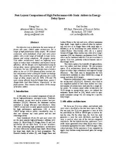
To see how this network can be constructed, consider the following iterative construction, shown in Figure 12

.

The basic building block of the construction is a chain of h-1 nodes. The nodes are indexed n(i,j), where i is the iteration count and j is the count of the nodes in the chain. At any iteration i, there is a source s(i,0) which is attached directly to node n(i,1). Each of the nodes n(i,j), j=1,2,...h-2 also have kh input links each, and all nodes n(i,j), j=2,...h-1 have hk output links. Each of input links of iteration i are connected to node n(i-1,4) of a network constructed at iteration i1 (the networks constructed at iteration i-1 are denoted S(i-1, j, m), where j is the index of the node in the chain, and m is the index of the input to node n(i, j) . That is, for each node n(i,j) of iteration i, hk black circles represent kh networks constructed at step i-1. Each of the kh output links corresponding to each node n(i,j) is connected to kh destination nodes, denoted D(i,j,m).

n(i,1)

n(i,2)

n(i,3)

n(i,4)

ra f

S(i,0)

S(i-1,3,3)

t

S(i-1,1,1) S(i-1,1,3) S(i-1,2,3)

D(i,2,1)

D(i,2,3)

D(i,4,1)

D(i,4,3)

Figure 12 The i-th iteration network. Black circles denote the networks constructed at step i-1. In this picture h=5 (which corresponds to 4 nodes in the chain). Only 3 of the kh i-1-level networks corresponding to each node n(i,j), j=1,2,3 are shown. Likewise, only 3 of the hk destination nodes corresponding to each node n(i,j), j=2,3,4, are shown. The flow sourced at node S(i,0) traverses the h-1 hop of the chain of iteration i. Once this flow exists node n(i,4), it is “plugged in” to one of the black nodes of iteration i+1, where it traverse its last hop along one of the links of the chain of iteration i+1.

At iteration

i=1 , each of the networks S(0,j,m) is just a single source node. Assume that all packets are the same

D

αC - and burst (depth) equal size, and that all the sources in the network are leaky bucket constrained with rates r = -------------kh + 1

to one packet. Assume that a flow originating at source S(0,

j, m) enters at node n(1, j) of the chain, traverses a

single hop of the chain and exits at node n(i, j+1) to destination D(0, j+1, m). Assume further that a flow originating at source s(1,0) traverses the whole chain. Note that the utilization of any link in the chain is precisely equal to α . Assume that the propagation time of any link is negligible (it will become clear that this assumption does not lead

to any loss of generality). Assume also that all links are of the same speed, and that the time to transmit the packet at link speed is chosen as unit of time. Assume that at iteration i=1 at time t=0 a single packet fully arrives to node n(1,1) from each of the sources S(1,1,m). Let’s color these packets blue. Assume also that at time zero a red packet started its transmission from node S(1,0) and fully arrived to n(1,1) at time t1=1. By this time one blue packet has arrived, and therefore the red packet has found a queue of length kh-1 blue packets ahead of it. By time t2=t1+kh the red packet will be fully transmitted from node n(1,1).


Page 25 of 31

A. Charny


Assume that at time t2-1 a single blue packet fully arrives from each of the nodes S(1,2,m), so that the red packet finds a queue of size kh-1 at the second node in the chain as well (recall that all the blue packets from the previous node exit the network at node n(1,2). Repeating this process at each of the nodes in the chain, it is easy to see that the red packet will suffer the total queueing delay of (h-1)(hk-1) packet-times. Since the rate of the red flow is

1 αC kh + 1 C C r = --------------- > --------------- ⋅ ------------ ⋅ --------------- = ------------------------------------- , it means that in (h-1)(hk-1) packet times at link speed C at least ( h – 1 ) ( kh – 1 ) kh + 1 kh – 1 h – 1 kh + 1

one more red packet can be transmitted from the source S(1,0). Since there are no other blue packets arriving to the

chain by construction, the second red packet will catch up with the first red packet, and hence the burst of at least two red packets will accumulate at the exit of node n(1,h-1). The next step of the iterative construction will take (h-1)hk of the networks constructed in step 1and connect the node n(1, 4) of each of these networks to one of the sources S(i-1, j, m) of the chain of the next iteration i=2. Let T(1) be the time it takes to accumulate the two-packet burst at the exit from node n(1, h-1) at iteration 1. Let then T(1) be the time when the first bit of the two-packet burst arrives at node n(2,1) from each of the nodes S(1,1,m). Let’s recolor all those packets blue. If the source S(2,0) emits a red packet at time t1=T(1)+1, then it fully arrives at node n(2,1) at

t

time t2=T(1)+2, and finds the queue equal to 2hk-1 blue packets (since 2hk packets have arrived and one has left in the previous time slot. That means that the last bit of the red packet will leave node n(2,1) at time T(1)+2+2kh. Assume now that the level-zero networks connected to node n(2,2) are started at time 2kh, instead of at time zero. This means

ra f

that by the time the last bit of our red packet arrives to node n(2,2), a two-packet (blue) burst will arrive to node n(2,2) from each of the networks S(1,2,m), and so the red packet will again find the queue of size 2kh-1 blue packets. Repeating this process for all h-1 nodes in the chain at iteration 2, we make the red packet delayed by (2kh-1)(h1)>2(kh-1)(h-1) packet times. During this time 2 more red packets will catch up, resulting in a 3-packet burst. Repeating this process as many times as necessary, we can grow a burst of red packets by one at each new iteration. Therefore, for any value of the delay D, we can always build a network of enough iterations, so that the burst B accumulated by the red flow over h-1 hops is such that B/C > D. Hence, taking one more iteration, it is easy to see that the red packet at the next iteration will be delayed by more than D at the first hop.

kh + 1 Note that choosing k large enough, --------------- can be made arbitrarily close to one, and so the example above implies 1 h–1

kh – 1

that for any α > ------------ and for any D>0 it is possible to choose large enough k and to construct a network with the worst

D

case delay exceeding D.

An interesting implications of this example is that the delay of a packet of a flow may be affected by flows which

do not share any links in common with the given flow, and what is even more surprizing, those flow had exited the network long before the flow to which the packet belongs has entered.

5.0 Summary and Discussion. This document has discussed the worst case delay in an network with aggregate scheduling . One of the

contributions of this paper has been to give a lower bound on the worst case delay and to demonstrate that it can be much larger than generally assumed. For a class of topologies an upper bound on the delay is also given. It has been shown that for this class of topologies there exists an area in parameter space where tight delay upper bounds on the worst case delay are possible with reasonable utilization numbers. The primary factors affecting the delay are the degree of aggregation and the quality of ingress shapers.


Page 26 of 31

A. Charny


While the class of networks satisfying this constraint is quite large, unfortunately in the general case this constraint is not satisfied. It turns out that it is possible to give an upper bound on the delay as a function of h and alpha for 1 C α < -------------------------------------------- , which, for C » S is α < ------------ [8]. However, unfortunately the bound in [8] explodes as ( C – S )( h – 1 ) – S h–1

1 1 α → ------------ . The results of this document imply that in fact for any α > ------------ the delay bound cannot be only a function h–1 h–1 of h and α : the delay bound, if it exists, must somehow depend on the size of the network. Determination of such 1 bounds for α > ------------ for an arbitrary network configuration remains an open problem. h–1

It is important to emphasize that the “average” behavior of the network may be substantially better than the worst case results described in this paper. However, at the present time characterizing the average behavior is a difficult challenge both for the engineering and the scientific community. The major challenge on the way to such characterization is the absence of adequate modelling of traffic patterns, routes and topology of the network. Such modelling is in itself a difficult problem which has not been well understood.

t

Acknowledgements.

The author is grateful to Jean-Yves Le Boudec and Jim Roberts for pointing out a flaw in the original version of

ra f

Theorem 1. Special thanks to my colleagues Bruce Davie, Francois Le Faucheur and Carol Itturalde for their helpful comments in preparation of this paper.

References.

F. Baker, C. Iturralde, F. Le Faucheur, B. Davie. Aggregation of RSVP for IPv4 and IPv6 Reservations, draft-ietf-issll-rsvp-aggr-00.txt, September 1999.

[2]

Schenker, S., Partridge, C., Guerin, R. Specification of Guaranteed Quality of Service, RFC 2212 Sep tember 1997

[3]

D. Oran. “Voice Over IP”, SIGCOMM’99 Tutorial-M1, August 1999

[4]

V. Jacobson, K. Nichols, K. Poduri. An Expedited Forwarding PHB, RFC 2598, June 1999.

[5]

J. Golestani, “A Self-Clocked Fair Queuing Scheme for Broadband Applications.” Proc. IEEE INFOCOM’94, 1994

D

[1]

[6]

J. Bennett, H. Zhang, “Hierarchical Packet Fair Queueing Algorithms” Proc. ACM SIGCOMM 96, 1966

[7]

Y. Bernet et.al, “A Framework For Integrated Services Operation Over Diffserv Networks”, draft-ietf-isslldiffserv-rsvp-03.txt, Sept. 1999

[8]

Jean-Yves Le Boudec. A proven delay bound for a network with Aggregate Scheduling. EPFL-DCS Technical Report DSC2000/002, http://ica1www.epfl.ch/PS_files/ds2.pdf


Page 27 of 31

A. Charny


Appendix A. The proof of Theorem 1 is based on the following two simple observations which allow iterative estimation of the burst accumulation and delay. Statement 1. If the maximum delay a packet of a flow can experience in a node is bounded by some D, then, if a flow is constrained by a leaky bucket with rate r and depth (burst) b at the entry to the node, then it is constrained by a leaky bucket (r, b+Dr) at the exit from this node. Statement 2. If all flows are constrained by leaky buckets at the entry to a queue with service rate S and service deficit bound β , and if the total input rate of all flows sharing the class queue does not exceed the service rate S, then the maximum delay of any packet at an output interface is bounded by

∑ b(i) + β

(22)

t

i D = -------------------------S

ra f

where b ( i ) is the leaky bucket depth of flow i, and the sum is taken among all flows sharing the output interface. Here, as before, flows can be either individual microflows flows or some aggregates of flows, where aggregation is allowed only among flows sharing the same ingress-egress pair. Proof of Statement 1.

Consider an arbitrary interval of time ( t 1 ,t 2 ) in which some number of bits were transmitted over the output interface. Let’s color all these bits red. Let τ 1 and τ 2 denote the arrival times of the first and the last bits of all the red bits. Since it is known that no packet is delayed by more than time D, and since no bit can be transmitted before it arrives, it must be the case that

D

and

τ1 ≤ t1 ≤ τ1 + D

(23)

τ 2 ≤ t2 ≤ τ 2 + D

(24)

Also, since the flow is constrained by a leaky bucket (r,b) at the entry to the hop, then the number B of red bits

arriving between τ1 and τis 2 bounded by B ≤ ( τ 2 – τ1 )r + b

(25)

From (23) and (24) we get τ 2 – τ 1 ≤ t 2 – ( t 1 – D ) = ( t 2 – t 1 ) + D , which together with (25) implies that at most B ≤ ( t 2 – t 1 )r + Dr + b bits could be transmitted over the outgoing link. Statement 1 now directly follows from the definition of a leaky bucket. Q.E.D. Proof of Statement 2.


Page 28 of 31

A. Charny


Let t be the time of arrival of some packet to the class queue at an output interface. Let’s color this packet red. Let t o ≤ t be the beginning of the queue busy period, which contains time ta . Without loss of generality assume t o = 0 .

Suppose the red packet is still in the queue at some time (26)

t = ta + D

Since the data of the same queue is served in FIFO order, only those bits that arrived before time t a could leave prior to the red packet. There could be at most A ( t a ) ≤ ∑ ( r ( i )t a + b ( i ) ) ≤ αSt a + ∑ b ( i ) i

(27)

i

t

of those bits (here α is the maximum class utilization factor allowed on any link). On the other hand, since the queue was constantly busy in the interval (0,t), by definition of the service deficit bound at least L ( t ) ≥ St – β

(28)

ra f

bits of priority traffic must have left by time t. Therefore, in order for the red packet to remain in the queue at time t, it must be that

A ( ta ) – L ( t ) ≥ 0 .

(29)

From (26), (27) and (28), (29) can be rewritten as

0 ≤ A ( t a ) – L ( t ) ≤ αSta + ∑ b ( i ) – St + β ≤ ∑ b ( i ) + β – SD + St a ( α – 1 ) ≤ ∑ b ( i ) + β – SD , i

i

(30)

i

The last inequality in (30) is true since α ≤ 1 . Therefore, (30) implies that

D

∑ b(i) + β

i D ≤ -------------------------S

(31)

(31) gives the bound on the maximum queueing delay. Q.E.D. To prove the statement of the Theorem an additional lemma will be needed. Lemma 1. For any flow traversing an h-degree hop in a network satisfying the monotonic degree constraint

the leaky bucket burst parameter at the exit from this hop h

is bounded by B h ( i ) ≤ b ( i ) + r ( i ) ∑ D j , where D j is the delay bound at a hop of degree j . Proof of Lemma 1.

j=1

This lemma is proved by induction on the degree of the hop. The base case is given by Statement 1. To prove the inductive step, assume that for any hop of degree k ≤ h – 1


Page 29 of 31

A. Charny


k

Bk ( i ) = b ( i ) + r ( i ) ∑ Dj

(32)

j=1

Consider a hop of degree h. By the monotonic degree assumption it means that the previous hop of any flow i entering the hdegree hop is of degree k ≤ h – 1 . By the inductive hypothesis it means that the burst parameter of the leaky bucket of any flow i entering the h-degree hop is bounded by (32). Since all delay bounds and rates are positive numbers, it is easy to see that h–1

k

Bk ( i ) = b ( i ) + r (i ) ∑ D j ≤ b ( i ) + r ( i ) ∑ D j j=1

(33)

j=1

Applying (33) as the input burst parameter of the leaky bucket in Statement 1 at hop of degree h+1completes the proof of the Lemma. Q.E.D.

t

Proof of Theorem 1.

It will now be shown by induction on the degree of the hop that the delay at a hop of degree h satisfies h – 1 ⎛ αb m ax

ra f Dh ≤ (1 + α )

--------------- + Δ⎞ ⎝ r min ⎠

(34)

To show the base case for (34), consider a hop of degree 1. By Statement 2 the max queue that a packet can experience in a first-degree hop is

∑ b(i) + β

nb max β αSb m ax βj αb max i D 1 ≤ -------------------------≤ --------------- + --- ≤ ------------------- + max j ⎛ ---- ⎞ = --------------- + Δ ⎝ S j⎠ S S S r min S r m in

(35)

which follows from the fact that the number n of flows in a queue with service rate S and utilization α cannot exceed

D

αS ---------- . This completes the proof of the base case. r min

To show the inductive step, suppose that (34) holds for all j ≤ h . It will now be shown that it also holds for

j = h + 1 . Consider any flow i sharing the hop of degree h+1. By definition of the degree of the hop, it must be the

case that the previous hop of flow i is of degree h or smaller. Therefore, by Lemma 1, the burst parameter of the leaky bucket of flow i at the entry to the hop of degree h+1 is bounded by h

B(i) ≤ b(i) + r(i)

∑ Dj

(36)

j=1

Therefore, by Statement 2 and the inductive hypothesis the queue at the h+1-st degree hop is bounded by h h ⎛ ⎞ αb 1⎜ j – 1 ⎛ αb max max ⎟ --------------- + Δ⎞ + Δ D j + 1 ≤ --- ∑ b ( i ) + ∑ r ( i ) ∑ D j + β ≤ --------------- + α ∑ ( 1 + α ) ⎝ r m in ⎠ ⎜ ⎟ S r mi n ⎝ ⎠ i j=1 j=1


Page 30 of 31

(37)

A. Charny


The second inequality here follows from (35) and from the fact that αb max αb max D j + 1 ≤ ⎛ --------------- + Δ⎞ + α ⎛ --------------- + Δ⎞ ⎝ r mi n ⎠ ⎝ r mi n ⎠

∑ r ( i ) ≤ αS . Now, (37) can be rewritten as i h

∑ (1 + α )

j–1

(38)

j=1

Summing up the geometric progression in (38), it can be rewritten as h αb max αb m ax (1 + α) – 1 h D h + 1 ≤ ⎛ --------------- + Δ⎞ ⎛ 1 + α ⎛ -----------------------------⎞ ⎞ = ⎛ --------------- + Δ⎞ ( 1 + α ) . ⎝ (1 + α) – 1 ⎠ ⎠ ⎝ r mi n ⎠⎝ ⎝ r min ⎠

(39)

This completes the inductive step for the proof of (34). To prove the statement of Theorem 1 it remains to note that a flow in a network satisfying the monotonic degree constraint can at most traverse one hop of each degree j=1,2...h, where h is the max hop count of any flow. Therefore,

D

ra f

t

the statement of theorem 1 can be immediately derived by summing (34) for all degrees from 1 to h.


Page 31 of 31

Delay Bounds In a Network With Aggregate ... - Semantic Scholar

Delay Bounds In a Network With Aggregate ... - Semantic Scholar

Suggest Documents

A Delay Bound for a Network with Aggregate Scheduling - Infoscience

Throughput and Delay Bounds for Cognitive ... - Semantic Scholar

Delay Line as a Chemical Reaction Network - Semantic Scholar

Creation of a Vehicular Delay-Tolerant Network ... - Semantic Scholar

A Delay-Tolerant Potential-Field-Based Network ... - Semantic Scholar

Creation of a Vehicular Delay-Tolerant Network ... - Semantic Scholar

Predictive Factors of Delay in Contact with a ... - Semantic Scholar

VoIP Network Dimensioning using Delay and Loss Bounds for Voice ...

A Dictyostelium mutant with defective aggregate ... - Semantic Scholar

Delay-Limited Cooperative Communication with ... - Semantic Scholar

A Dictyostelium mutant with defective aggregate ... - Semantic Scholar

A Case for Aggregate Networks - Semantic Scholar

Delay Space - Semantic Scholar

delay discounting? - Semantic Scholar

Bounds on the Throughput Gain of Network ... - Semantic Scholar

Aggregate Predicate Support in DBMS - Semantic Scholar

Trends in Aggregate Vehicle Emissions - Semantic Scholar

Multiproduct aggregate production planning in ... - Semantic Scholar

Locality-Based Aggregate Computation in ... - Semantic Scholar

Transparent Autonomization in Aggregate Web ... - Semantic Scholar

On Delay Performance Gains From Network Coding - Semantic Scholar

Delay Tolerant Network on Android Phones - Semantic Scholar

Queuing Network Models for Delay Analysis of ... - Semantic Scholar

Where the Network ends: Infrastructure and Delay ... - Semantic Scholar