Jul 20, 2012 - Abstract: The theory of non-commutative rings allows determining whether ... Keywords: Nonlinear Time delay system, Time delay estimation, ...
Author manuscript, published in "IFAC TDS (2012)"
Delay estimation algorithm for nonlinear time-delay systems with unknown inputs J.-P. Barbot ∗ G. Zheng ∗∗ T. Floquet ∗∗∗ D. Boutat ∗∗∗∗ J.-P Richard † ∗
hal-00719761, version 1 - 20 Jul 2012
ECS-Lab ENSEA, Cergy-Pontoise, 95014, France and EPI Non-A, INRIA. ∗∗ Project Non-A, INRIA Lille-Nord Europe, 40, avenue Halley, 59650 Villeneuve d’Ascq, France ∗∗∗ Project Non-A, INRIA Lille-Nord Europe, 40, avenue Halley, 59650 Villeneuve d’Ascq, France ∗∗∗∗ Loire Valley University , ENSI-Bourges, Institut PRISME, 88 Bd. Lahitolle, 18020 Bourges Cedex, France † Project Non-A, INRIA Lille-Nord Europe, 40, avenue Halley, 59650 Villeneuve d’Ascq, France Abstract: The theory of non-commutative rings allows determining whether or not there exists an equation called algebraically essential in order to estimate the delay on a nonlinear system. In this paper, it firstly recalls some literature results on algebraically essential equation. Then it is shown that this equation is generally not enough to guarantee the delay estimation, thus the notion of persistent signal with respect to delay estimation is introduced. Furthermore, based on the definitions of algebraically essential equation and of persistent signal, a delay estimation algorithm is proposed. Some simulation results have been presented in order to highlight the robustness (with respect to measurement noise) of the proposed algorithm. Keywords: Nonlinear Time delay system, Time delay estimation, Algebraic approach 1. INTRODUCTION Time-delay systems are widely used to model concrete systems in engineering sciences, such as biology, chemistry, mechanics and so on Kolmanovskii and Myshkis (1999); Niculescu (2001); Richard (2003). Among all, delay estimation is one of the important topics in the field of timedelay systems. Up to now, various techniques have been proposed for the delay identification problem, such as identification by using variable structure observers Drakunov et al., by a modified least squares technique Ren et al. (2005), by convolution approach Belkoura (2005), by using the fast identification technique proposed in Fliess and Sira-Ramirez (2004) to deal with online identification of continuous-time systems with structured entries Belkoura et al. (2009) and so on. Our previous work in Zheng et al. (2011) proposed necessary and sufficient conditions to deduce an essential algebraic equation (which will be recalled in the next section) for nonlinear time delay systems with unknown inputs, which can be used to estimate the corresponding time delay. This paper presents a delay estimation algorithm for the deduced essential equation based on the results of Zheng et al. (2011). The work of this paper can be seen as a further study of Zheng et al. (2011) by proposing an optimization method to estimate the delay. Unlike many existing methods in the literature which are generally for linear time delay system (see for example Bj¨orklund and
Ljung (2003)), the proposed algorithm works as well for nonlinear time delay systems. Moreover, this algorithm is robust with respect to noise. This paper is organized as follows. Section 2 recalls some necessary elements involved in this paper, which are given in Xia et al. (2002) and Zheng et al. (2011). The delay estimation algorithm is presented in Section 3, and an illustrative example and the corresponding simulations are given in Section 4 to highlight the proposed algorithm. 2. RECALL OF NECESSARY ELEMENTS The proposed delay estimation algorithm of this paper is based on the algebraic framework introduce in Xia et al. (2002), and is an extension result of Zheng et al. (2011). Therefore, before stating the main result, it is necessary to recall the involved elements. 2.1 Algebraic framework Let denote τ the basic time delay, and assume that the times delays are multiple times of τ . Consider the following nonlinear time-delay system: s ∑ g j (x(t − iτ ))u(t − jτ ) x˙ = f (x(t − iτ )) + j=0
y = h(x(t − iτ )) = [h1 (x(t − iτ )), . . . , hp (x(t − iτ ))]T x(t) = ψ(t), u(t) = ϕ(t), t ∈ [−sτ, 0] (1)
hal-00719761, version 1 - 20 Jul 2012
where x ∈ W ⊂ Rn denotes the state variables, u = [u1 , . . . , um ]T ∈ Rm is the unknown admissible input, y ∈ Rp is the measurable output. Without loss of generality, we assume that p ≥ m. And i ∈ S− = {0, 1, . . . , s} is a finite set of constant time-delays, f , g j and h are meromorphic functions 1 , f (x(t − iτ )) = f (x, x(t − τ ), . . . , x(t − sτ )) and ψ : [−sτ, 0] → Rn and ϕ : [−sτ, 0] → Rm denote unknown continuous functions of initial conditions. In this work, it is assumed for initial conditions ψ and ϕ, (1) admits a unique solution. Based on the algebraic framework introduced in Xia et al. (2002), let K be the field of meromorphic functions of a finite number of the variables from {xj (t−iτ ), j ∈ [1, n], i ∈ S− }. With the standard differential operator d, define the vector space E over K: E = spanK {dξ : ξ ∈ K} which is the set of linear combinations of a finite number of one-forms from dxj (t − iτ ) with row vector coefficients in K. For the sake of simplicity, we introduce backward time-shift operator δ, which means δ i ξ(t) = ξ(t − iτ ), ξ(t) ∈ K, for i ∈ Z + (2) and δ i (a(t)dξ(t)) = δ i a(t)δ i dξ(t) (3) = a(t − iτ )dξ(t − iτ ) for a(t)dξ(t) ∈ E, and i ∈ Z + . Let K(δ] denote the set of polynomials of the form (4) a(δ] = a0 (t) + a1 (t)δ + · · · + ara (t)δ ra where ai (t) ∈ K. The addition in K(δ] is defined as usual, but the multiplication is given as r∑ a ,j≤rb a +rb i≤r∑ a(δ]b(δ] = ai (t)bj (t − iτ )δ k (5) k=0
i+j=k
Note that K(δ] satisfies the associative law and it is a noncommutative ring (see Xia et al. (2002)). However, it is proved that the ring K(δ] is a left Ore ring Jeˇzek (1996); Xia et al. (2002), which enables to define the rank of a module over this ring. Let M denote the left module over K(δ]: M = spanK(δ] {dξ, ξ ∈ K}, where K(δ] acts on dξ according to (2) and (3). With the definition of K(δ], (1) can be rewritten in a more compact form as follows: m ∑ Gi ui (t) x˙ = f (x, δ) + (6) i=1 y = h(x, δ) x(t) = ψ(t), u(t) = ϕ(t), t ∈ [−sτ, 0] where f (x, δ) = f (x(t − iτ )) and h(x, δ) = h(x(t − iτ )) ∑s with entries belonging to K, Gi = j=0 gij δ j with entries belonging to K(δ]. 2.2 Notations and Definitions Let f (x(t−jτ )) and h(x(t−jτ )) for 0 ≤ j ≤ s respectively be an n and p dimensional vector with entries fr ∈ K for 1 ≤ r ≤ n and hi ∈ K for 1 ≤ i ≤ p. Let ] [ ∂hi ∂hi ∂hi ∈ K1×n (δ] (7) = ,··· , ∂x ∂x1 ∂xn 1 means quotients of convergent power series with real coefficients Conte et al. (1999); Xia et al. (2002).
where for 1 ≤ r ≤ n: s ∑ ∂hi ∂hi = δ j ∈ K(δ] ∂xr ∂x (t − jτ ) r j=0 then the Lie derivative for nonlinear systems without delays can be extended to nonlinear time-delay systems as it was first proposed by Oguchi et al. (2002). Our extension is based on the framework of Xia et al. (2002) as follows: s n ∑ ∑ ∂hi ∂hi L f hi = (f ) = δ j (fr ) ∈ K (8) ∂x ∂x (t − jτ ) r r=1 j=0 For j = 0, (8) is the classical definition of the Lie derivative of h along f . For hi ∈ K, define ∂hi (Gi ) ∈ K(δ] L Gi h i = ∂x After having defined the derivative of function belonging to K(δ], let study the time delay identification for system (6). Definition 1. An output equation α(h, h˙ . . . , h(k) , δ) = 0 (9) is said to involve δ in an essential way if it cannot be written as α(h, h˙ . . . , h(k) , δ) = a(δ]α ˜ (h, h˙ . . . , h(k) ) with a(δ] ∈ K(δ]. As stated in Anguelova and Wennberg (2008), if there exists a function for (6) containing only the output, its derivatives and delays in an essential way, then the delay can be identified by numerically finding zeros of such a function. Thus delay identification for (6) becomes to seek such a function. Remarks 1. Existence of equation (9) is not enough to guarantee the possibility to estimate the delay δ. For examples: • if h, h˙ . . . , h(k) are equal to zero for all t > −τ , equation (9) is equal to zero for all τ . • if the signal h is periodic of period T , it is only possible to detect τ ∈ [0, T [. 2.3 Identifiability In order to estimate the time delay for (6), one needs to derive essential equation from (6) which in fact is equivalent to study the delay identifiability of (6). Our previous work in Zheng et al. (2011) has given necessary and sufficient conditions to seek the essential equation for nonlinear time delay systems. Generally speaking, two cases are possible. The simplest case is to estimate the delay from only the outputs of (6). This implicitly means that the output of (6) is dependent over K(δ], and the deduced essential equation from the outputs can be used directly to estimate the delay. The complicated case is that the output of (6) is independent over K(δ], i.e., rankK(δ] ∂h ∂x = p, and this needs to analyze the dynamics of the studied systems. Necessary and sufficient condition for the simplest case has been given in Theorem 1 in Zheng et al. (2011). For the second case, sufficient condition can be found in Zheng et al. (2011) (Theorem 3) in order to guarantee the existence of a function containing only the output, its derivatives and delays. Theorem 4 of Zheng et al. (2011)
stated necessary and sufficient condition to check whether the deduced function can be used to estimate the delay. Since the aim of this paper is to propose delay estimation algorithm based on our previous work in Zheng et al. (2011), in order to avoid the redundance, interested reader can refer to Zheng et al. (2011) for those results. 3. DELAY ESTIMATION ALGORITHM
hal-00719761, version 1 - 20 Jul 2012
In this paper, only local estimation of the time delay τ is investigated. Moreover, we restrict the time delay by making the following assumption. Assumption 1. The time delay τ for the studied system is considered to be constant or sufficiently slowly variable with respect to the delay estimation process. It is well-known that the persistent exciting condition in parameter estimation is necessary. In this paper, the same assumption is imposed as well, i.e. it is supposed that the signal is sufficiently persistent with respect to the essential algebraic equation. It is worthy noting that the notion of persistent signal is close to that of persistent input Dufour et al. (2010) (quite different from the universal input Gauthier and Bornard (1981)) in observation problem or persistent excitation Narendra and Annaswamy (1987) in adaptive problem. Definition 2. The signal is sufficiently persistent with respect to the equation (9) for the interval of delay uncertainty [0, T [, if there exists a bounded θ > 0 such that there exists one and only one τ ∈ [0, T [ such that ∫ θ (α(h, h˙ . . . , h(j) , τ ))2 dt = 0 0
For the sake of notation simplicity , the essential equation α is indifferently noted in function of the operator δ or the time delay τ . So, based on Definitions 1 and 2, it is thus possible to design a delay estimation algorithm. In this paper, only an algorithm based on the classical descent optimization method is given in order to highlight the result proposed in Zheng et al. (2011) according to Definitions 1 and 2 given above. Nevertheless, it is important to mention that the proposed algorithm is robust to noise, and can be used to estimate time delay for nonlinear time delay system, since many existing delay estimation algorithms in the literature are generally for linear process (see Bj¨orklund and Ljung (2003) and the reference therein). This restriction to linear estimation is principally due to: • In nonlinear case, the estimated time delay is generally only a local extremum solution. In the algorithm presented below, this problem is overcome by adding a random process. • For nonlinear equation, a noisy signal will normally introduce a bias. For example, considering y a signal and η a Gaussian noise, then E(y + η) is equal to E(y), but E((y+η)2 ) is not equal to E(y 2 ). This theoretical difficulty is overcome in the algorithm proposed below due to the fact that an exact solution of the essential equation is not expected. More precisely, if E(α(y,˙, .., τe + η)2 ) is smaller than E(α(y,˙, .., τw )2 ) where τe is the exact estimate delay and τw is a wrong estimate delay, our algorithm work, this sets the problem of estimation precision with respect to the noise.
For the sake of simplicity, hereafter, it is assumed that the unknown time delay τL is a multiple of a known minimum delay τm (thus τL = Li τm where Li ∈ N is the unknown integer to be identified) and there exists also a maximum expected delay τM = LM τm with LM ∈ N and bounded. Then, the delay estimation algorithm can be stated as follows. Step 1: (Initialization step) At time t = 0, initial values L0 and Lr are obtained from a random number generator, where L0 and Lr are chosen in the set {0, 1, ..., LM }. Step 2: For t ∈]0, θ[, where θ is the time integration frame (θ is chosen with respect to Definition 2), the following integrals are computed: ∫ θ I(L0 ) = α(h, h˙ . . . , h(j) , L0 τm )2 dt 0
I(L0 ) =
∫
I(L¯0 ) =
∫
I(Lr ) =
∫
θ
α(h, h˙ . . . , h(j) , L0 τm )2 dt
(10)
0 θ
α(h, h˙ . . . , h(j) , L¯0 τm )2 dt
0 θ
α(h, h˙ . . . , h(j) , Lr τm )2 dt
0
where L0 is the max of L0 − 1 and 0; L¯0 is the min of L0 + 1 and LM . The objective for introducing those different integrals is to overcome the estimation overflow. Step 3 (2k + 1 with k = 1): At time t = θ, L1 is taken equal to the value of the set {L0 , L0 , L¯0 , Lr } which minimizes I(.) in (10) and a new Lr is randomly chosen. Step 4 (2k + 2 with k = 1): For t ∈]θ, 2θ[=]kθ, (k + 1)θ[ (with k = 1), the following integrals are computed: I(L1 ) =
∫
I(L1 ) =
∫
I(L¯1 ) = I(Lr ) =
∫ ∫
θ 0 θ
α(h, h˙ . . . , h(j) , L0 τm )2 dt α(h, h˙ . . . , h(j) , L0 τm )2 dt
(11)
0 θ
α(h, h˙ . . . , h(j) , L¯0 τm )2 dt
0 θ
α(h, h˙ . . . , h(j) , Lr τm )2 dt
0
where L1 is the max of L1 − 1 and 0; L¯1 is the min of L1 + 1 and LM .
Recursively Step 2k + 1: At time t = kθ, Lk is taken equal to the value of the set {Lk-1 , Lk−1 , Lk−1 ¯ , Lr } which minimizes I(.) and a new Lr is randomly chosen. Step 2k + 2: For t ∈]kθ, (k + 1)θ[, the following integrals are computed:
I(Lk ) =
∫
I(Lk¯ ) = I(Lr ) =
θ 0
2
(α(h, h˙ . . . , h(j) , Lk τm )2 dt
1.5
θ
(α(h, h˙ . . . , h(j) , (Lk )τm )2 dt
(12)
0 θ
∫
∫0
(α(h, h˙ . . . , h(j) , Lk¯ τm )2 dt
θ(α(h, h˙ . . . , h(j) , (Lr τm )2 dt
1 y1 in red and y2 in Blue
I(Lk ) =
∫
0.5
0
−0.5
0
where Lk is the max of Lk − 1 and 0; Lk¯ is the min of L1 + 1 and LM .
−1
−1.5
0
0.1
0.2
0.3
0.4
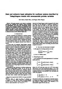
The simulation results for different scenarios are depicted in Fig. 1-6, and one can draw the following conclusions. • Fig. 1 and Fig. 2 show respectively the outputs y1 , y2 and the delay estimation for system without noise, in this case the proposed algorithm works satisfactorily. • Fig. 3 and Fig. 4 show respectively the outputs y1 , y2 and the delay estimation in the case of correlated noise η (Gaussian noise of power 0.001). For these simulations, the measured output y2,mesured is equal to (y1 + η)δ(y1 + η) + (y1 + η)2 and the measured output y1,measured is equal to y1 + η. In this case, the noise power has no influence on the delay detection as it is shown in Fig 4. This is due to the fact that the essential equation is also verified by y1 + η. Nevertheless, this case is unrealistic and hereafter a uncorrelated noises will be considered. • Fig. 5 and Fig. 6 show the result with correlated noises. In this case the measured output y2,mesured is equal to (y1 δy1 +(y1 +)2 +η2 and the measured output y1,measured is equal to y1 + η1 with η1 and η2 to uncorrelated gaussian noises of power
0.7
0.8
0.9
1
0.6
0.7
0.8
0.9
1
0.8
0.9
1
0.045
0.04
0.035
0.03
0.025
0.02
0.015
0.01
0.005
∂h which yields rankK(δ] ∂h ∂x = 1 and rankK ∂x = 2. Thus Theorem 1 of Zheng et al. (2011) is satisfied, and the time delay of system (13) can be estimated.
For the simulation, τm is equal to 0.01s, τM is equal to 0.1s, the estimation time frame θ is equal to 0.1s and the delay to be estimated is 0.03s. Moreover, as it is shown in Fig 1 the outputs are sinusoidal but with a period greater than τmax , then the signals are sufficiently persistent with respect to the considered delay.
0.6
0.05
It can be seen that ( ) ∂h 1 0 = δx1 + 2x1 + x1 δ 0 ∂x
In fact, a straightforward calculation gives y2 = y1 δy1 + y12 which permits to estimate the time delay δ by applying the algorithm presented in the previous section.
0.5 time
Fig. 1. y1 and y2 without noise
estimated delay
In order to highlight the proposed algorithm, this section gives only a simple example for which delay can be estimated from only its output. For this, let consider the following dynamical system: x˙ = x2 + 10πx1 (1 − x21 − x22 ) 1 x˙ 2 = −x1 + 10πx2 (1 − x21 − x22 ) (13) y1 = x1 2 y2 = x1 δx1 + x1
0
0
0.1
0.2
0.3
0.4
0.5 time
Fig. 2. Delay estimation without noise 140
120
100
80 y1 in red and y2 in blue
hal-00719761, version 1 - 20 Jul 2012
4. SIMULATION RESULTS
60
40
20
0
−20
−40
0
0.1
0.2
0.3
0.4
0.5 time
0.6
0.7
Fig. 3. y1 and y2 with correlated noises 0.00001. For the considered system and delay estimation algorithm, this level of noise is an upper limit for correct delay detection. 5. CONCLUSION Our previous work of Zheng et al. (2011) gave necessary and sufficient conditions to deduce the essential equations for nonlinear time delay systems in order to estimate the corresponding delay. As a further work based on Zheng et al. (2011), this paper proposed a delay estimation algorithm based on the deduced essential equation by using optimization method. An illustrative example is
0.05
0.045
0.04
estimated delay
0.035
0.03
0.025
0.02
0.015
0.01
0.005
0
0
0.1
0.2
0.3
0.4
0.5 time
0.6
0.7
0.8
0.9
1
Fig. 4. Delay estimation with correlated noises 4
3
y1 in red and y2 in blue
1
0
−1
−2
0
0.1
0.2
0.3
0.4
0.5 time
0.6
0.7
0.8
0.9
1
0.8
0.9
1
Fig. 5. y1 and y2 with uncorrelated noises 0.05
0.045
0.04
0.035
estimated delay
hal-00719761, version 1 - 20 Jul 2012
2
0.03
0.025
0.02
0.015
0.01
0.005
0
0
0.1
0.2
0.3
0.4
0.5 time
0.6
0.7
Fig. 6. Delay estimation with uncorrelated noises presented as well to show the feasibility and robustness of the proposed delay estimation algorithm. Future works will be done to improve the identification algorithm, treating more than one delay and study the closed loop control based on the estimation of the state and delays. REFERENCES Anguelova, M. and Wennberg, B. (2008). State elimination and identifiability of the delay parameter for nonlinear time-delay systems. Automatica, 44(5), 1373–1378. Belkoura, L. (2005). Identifiability of systems described by convolution equations. Automatica, 41, 505–512.
Belkoura, L., Richard, J.P., and Fliess, M. (2009). Parameters estimation of systems with delayed and structured entries. Automatica, 45(5), 1117–1125. Bj¨orklund, S. and Ljung, L. (2003). A review of time-delay estimation techniques. Proc. 42nd IEEE Conf. Decision and Control, 2502–2507. Conte, G., Moog, C., and Perdon, A. (1999). Nonlinear control systems: An algebraic setting. Lecture Notes in Control and Information Sciences, 242, Springer– Verlag,London. Drakunov, S., Perruquetti, W., Richard, J.P., and Belkoura, L. (????). Delay identification in time-delay systems using variable structure observers. Annual reviews in control, 30(2), 143–158. Dufour, P., Flila, S., and Hammouri, H. (2010). Nonlinear observers synthesis based on strongly persistent inputs. Proc. IEEE Conf. Decision and Control. Fliess, M. and Sira-Ramirez, H. (2004). Reconstructeurs d’´etat. Comptes Rendus de l’Acad´emie des Sciences Series I, 338(1), 91–96. Gauthier, J.P. and Bornard, G. (1981). Observability for any u(t) of a class of nonlinear systems. IEEE Transactions on Automatic Control, 26(4), 922926. Jeˇzek, J. (1996). Rings of skew polynomials in algebraical approach to control theory. Kybernetika, 32(1), 63–80. Kolmanovskii, V. and Myshkis, A. (1999). Introduction to the theory and application of functional differential equations. Kluwer Academic Publishers, Dordrecht. Narendra, K.S. and Annaswamy, A.M. (1987). Persistent excitation in adaptive systems. International Journal of Control, 45(1), 127–160. Niculescu, S.I. (2001). Delay effects on stability: A robust control approach. Lecture Notes in Control and Information Sciences, Springer, 269. Oguchi, T., Watanabe, A., and Nakamizo, T. (2002). Input-output linearization of retarded non-linear systems by using an extension of lie derivative. Int. Jour. of Control, 75(8), 582–590. Ren, X., Rad, A., Chan, P., and Lo, W. (2005). Online identification of continuous-time systems with unknown time delay. IEEE Transaction on Automatic Control, 50(9), 1418–1422. Richard, J.P. (2003). Time-delay systems: an overview of some recent advances and open problems. Automatica, 39(10), 1667–1694. Xia, X., Marquez, L., Zagalak, P., and Moog, C. (2002). Analysis of nonlinear time-delay systems using modules over non-commutative rings. Automatica, 38, 1549– 1555. Zheng, G., Barbot, J.P., and Boutat, D. (2011). Delay identification for nonlinear time-delay systems with unknown inputs. Proc. of IEEE Conf. Decision and Control.