plicated case of varying service time, the MT minimization sheds light on the design of a simple scheduler. Overall, the marginal utility requires significantly low ...
1
Delay-Sensitive Packet Scheduling for a Wireless Access Link Young-June Choi and Saewoong Bahk, Member, IEEE
Abstract— As the delay is a critical QoS factor, packet scheduling over a wireless access link that often becomes congested needs to have the objective of meeting each user’s delay requirement. To incorporate the delay into the scheduler design, we consider the objective of maximizing the total utility (UT ). However, since a utility-based scheduler that concerns delay requires high complexity, we introduce the concept of marginal utility. Representing the objective as minimizing the total marginal utility (MT ), we develop some related properties for maximizing UT and minimizing MT . For the case with fixed service time, we show that the outcome of MT minimization becomes equivalent to that of UT maximization. For the more complicated case of varying service time, the MT minimization sheds light on the design of a simple scheduler. Overall, the marginal utility requires significantly low complexity for packet scheduling compared to the ordinary utility. Through simulations, we confirm that the marginal utility gives a way of flexible scheduling in meeting various delay requirements. Index Terms— communication networks, scheduling, marginal utility, delay, simulation
packet
I. I NTRODUCTION Nowadays, communication networks have been expanded owing to the technology of broadband networks and the deployment of wireless mobile networks. Broadband networks based on optical transmission technology enable users to access the Internet at high speed over tens of Mbps. Meanwhile, wireless networks such as wireless LANs have been deployed and cellular networks have also started data services. The available transmission speed reaches up to 54Mbps in IEEE 802.11a/g systems, and 2Mbps and 10Mbps in HDR (cdma2000 1x EV-DO) and WCDMA-HSDPA systems, respectively. Besides, wireless personal area networks and wireless metropolitan area networks have been standardized in 802.15 and 802.16 groups, respectively. A main feature of these This research was supported partially by the University IT Research Center Project and the Ubiquitous Autonomic Computing and Network Project, Ministry of Information and Communication, in Korea. Young-June Choi and Saewoong Bahk are with the school of EE and INMC, Seoul National University, Seoul, 151-742, Korea (Email: {yjchoi, sbahk}@netlab.snu.ac.kr)
wireless systems is in their IP centered architecture. Next generation mobile communication systems beyond 3G are expected to integrate all these networks with IP technology. In integrated networks, wireless links often become congested due to narrow bandwidth. Therefore, resource management for wireless access links becomes an important issue. Packet scheduling plays a key role in resource management. In conventional IP networks, each queue at a router focuses on achieving fairness by the weighted fair queueing (WFQ) scheduler [2] or its variants. To apply those schedulers to a wireless network, some works try to compensate for user’s location-dependency in bandwidth and burst channel error over the wireless link (See [1]). As a way of compensation, they simply classified the wireless channel into good or bad state, and used its state for scheduling decision. Recently opportunistic scheduling that exploits fading channels has been researched actively [11]–[15]. Although the opportunistic scheduling is beneficial to best-effort traffic in the physical layer, it cannot guarantee each user’s network-level QoS explicitly. Meanwhile, earliest deadline first (EDF) [3] scheduling is known to be optimal in meeting the delay bound at a single node [4]. It serves packets in ascending order of deadlines and guarantees per-flow quality of service (QoS). In [6], it was shown that EDF scheduling in conjunction with a fair discarding mechanism is effective in increasing network utilization. In the area of processor scheduling, the shortest remaining processing time (SRPT) scheme [7] has a concept opposite to that of EDF scheduling because it serves the packet with the shortest delay first. It is known that SRPT minimizes the average delay, but it has the drawback of starving packets with long processing time [8]. The authors in [8] compare the SRPT algorithm with the normalizeddelay algorithm for CDMA downlink. Recent works in packet scheduling have introduced the concept of utility. Shenker in [9] first applies the utility concept to the network area. Kelly derives proportional fairness for elastic-utility traffic based on the utility concept in [10]. In [11], the concept of proportional fairness is applied to HDR systems. Some works also investigate
Frequency
frame Channal 1 Channal 2 Channal 3 Channal 4
Time scheduling
scheduling (a)
Frequency
the general utility function for opportunistic scheduling or power control [14], [16]. Although the objective of the existing works has generally been maximizing the total utility, it is known in Economics that the total utility is inappropriate in explaining the decision activity [18]. Therefore we adopt the marginal utility as a different aspect of utility to get help for scheduling decision for delay-sensitive packets. In contrast to the previous works, we represent the utility as a function of delay to reflect various delay impacts. In our consideration, we classify the system into two types according to the multiplexing type. One is the single-server case that covers time division multiplexing, and the other is the multiple-server case that deals with frequency/code division multiplexing. Conventionally, real-time service in wireless networks has been implemented by the multiple-server type which guarantees target data rate for each user. To overcome channel fading, most cellular systems use some techniques like power control, which usually uses the frame structure of fixed service time. On the other hand, recent systems such as HDR and HSDPA exploit a single server and opportunistic scheduling instead of power control. That is, they take advantage of fading channel condition rather than compensate for it. In this case, the frame structure usually deals with varying service time. In future networks, realtime service will be partially supported by opportunistic scheduling [5], [12], [13], [17]. Therefore our system model includes both types: fixed service time for the multiple-server case and variable service time for the single-server case. We skip the case of variable service time for the multiple-server since it is just an easy extension of the above two types. In this paper, we investigate general delay-sensitive packet scheduling over a bottleneck, for instance a wireless access link, rather than opportunistic nature of wireless channels. In integrated networks including wireless LANs or cellular networks, the downlink queue at a base station (BS) often tends to be congested and dominates the delay in delivering delay sensitive packets. The issue of opportunistic scheduling with delay consideration is left for future work. The contributions of this paper are threefold. First, we introduce the concept of marginal utility to design our packet scheduling strategies for delay-sensitive traffic over an access link. Second, for the case with fixed service time, we show that the scheduling strategy of MT minimization is equivalent to that of UT maximization. Third, for the case with variable service time, we resolve UT maximization and MT minimization problems by a heuristic algorithm and an asymptotic algorithm, respectively. For any cases, MT minimization
frame
Time
slot scheduling
scheduling (b)
Fig. 1. Scheduling types according to multiplexing: (a) frequency division multiplexing; (b) time division multiplexing.
can be a useful objective for packet scheduling because of its simplicity in implementation. The rest of this paper is organized as follows. Section II describes our considered model and some basic disciplines about the marginal utility. Section III and IV consider scheduling objectives applicable to the case with fixed service time and variable service time, respectively. Finally, Section V shows simulation results, followed by conclusion in Section VI. II. M ARGINAL U TILITY A. Delay model We consider scheduling policies for delay-sensitive packets over an access link that often becomes a bottleneck. Although the actual delay felt by a user comprises of each queueing delay at a node through the network, the delay over the bottleneck link usually dominates the total end-to-end delay. Hence we define the system delay only over the access link.1 Representing the waiting time 1
Although the bottleneck link may exist over the network, the access link can be most likely the bottleneck due to the narrow wireless bandwidth.
in queue as queueing delay ω and the packet transmission duration as service time σ , we can write the system delay τ as the sum of both delays, that is, (1)
σ =
R X
pke (1 − pe ) ((k + 1)σo + kδ)
(2)
k=0
= (1 − pe )R+1 ((R + 1)(R + 2)σo + R(R + 1)δ) /2
where σo is the transmission time of a packet, and δ is the interval between packet transmission and reception of the corresponding ACK. Unlike this simple retransmission scheme, we can have further considerations for hybrid ARQ or its advanced versions [21], which we omit here because they are beyond the scope of this paper. When a frame starts, the scheduler selects packets that will be served within it. In case of FDM, the service delay for each selected packet equals the frame length, assuming the encoder for traffic stream generates a
Delay bound
Utility
When the transmission rate is constant, σ is the same for homogeneous traffic that means the traffic of same packet size. An example is code division multiplexing (CDM) that supports constant transmission rate with power control. If the transmission rate varies according to the channel condition, σ varies even for the same packet size. Such an example is time division multiplexing (TDM) without power control like in IEEE 802.11 and HDR. The queueing delay ω depends on the scheduling strategy and the multiplexing type. As shown in Fig. 1, we can classify the multiplexing type into frequency division multiplexing (FDM) and TDM. We put CDM into FDM type because CDM allows multiple users to transmit simultaneously by assigning a unique code for each user. In any cases, we assume that the average data rate remains constant during the transmission. Similar assumptions are used in [19] and [20]. If our scheduler coexists with some underlying channel-aware schedulers, the actual transmission sequence may not follow our scheduling result due to the opportunistic transmission or other diversity effects in the physical layer. However, for simple analysis, we assume the underlying physical-layer scheduling does not affect the delay of our network-level scheduling in a macroscopic scale. Also the retransmission effect in erroneous wireless environments can be included in the estimation of delay by counting the probabilistic retransmission. If we denote the estimated error probability as pe and the maximum number of retransmissions as R, the scheduler can estimate the service time as follows:
Delay
(a)
Delay-sensitive packet Delay-insensitive packet
Marginal Utility
τ = ω + σ.
Delay-sensitive packet Delay-insensitive packet
Delay
(b)
Fig. 2. Examples of utility and marginal utility function: (a) examples of utility functions; (b) marginal utility functions for (a).
constant bit rate. This scenario can be generally accepted for CDMA systems as well. In case of TDM, however, the service time is shorter than the frame length and the queueing delay varies according to the service sequence within the frame. If the service time is fixed as shown in Fig. 1 (b), slot-level scheduling can be considered as a special case of frame-level scheduling of FDM. Therefore, in this work, we analyze the scheduling strategy according to the service time: fixed service time and variable service time. B. Introduction to marginal utility To represent the level of satisfaction about goods or service, microeconomics has introduced the concept of utility. Usually the utility increases concavely in proportion to the received amount of goods or service. Similarly we can think about the utility function of system delay where the utility decreases with the increase of delay. From the utility theory, we adopt the following assumption.
Assumption 1: Utility has measurability and additivity. From the measurability assumption, we can depict the utility in terms of delay as shown in Fig. 2 (a). If packets are delay-sensitive, we can use a utility function that decreases concavely and falls down steeply near the delay bound. On the other hand, for delay-insensitive packets, the utility decreases convexly. Now we consider the total utility that can be obtained by packet scheduling. Assumption 2: Assume sessions have utilities independent of one another. Then we can write the total utility as the sum of each utility.2 That is, X U (; i) (3) UT = i∈Φ
where UT , U (; i), and Φ represent the total utility, the utility3 of session i, and the scheduled session4 set, respectively. As the scheduling strategy affects the total utility very much, we develop the optimal scheduling strategy that maximizes the total utility. Objective-I : max UT
(4)
The total utility, however, has no effect on helping the decision whether to buy one more unit of goods or not [18].5 This motivates us to consider another form of metric for scheduling decision; that is the marginal utility which has been interpreted by economists as the amount of utility gain or loss. In this paper we define it as the utility increase created by consuming one more unit of goods. Applying this for the utility of delay, we can generalize the marginal utility at i-th frame when the packet service is expected available at (i + k)-th frame as i+k X M (ω) = U (ω + ζj ) − U (ω + ζi ) (5) j=i
where U (t) and M (t) denote the utility and the marginal utility at time t, respectively, and ζi is i-th frame length. The utility is attained at ω +ζi if a packet is scheduled at the current frame. If scheduled at the next frame, it will have a utility value at ω + ζi + ζi+1 . As the frame length 2
This statement is not always true because of the characteristics of goods or service in microeconomics. 3 U (t; i) is the utility of session i at time t. If the time need not be specified, we represent it as U (; i). 4 One user may have several sessions at the same time and each session involves an active queue. 5 In spite of this, we use the total utility as an objective for comparative study.
is typically fixed, we can represent ζi as ζ . If the utility function is continuous and differentiable for some small ζ , we can obtain the marginal utility by differentiating it. That is, M=
dU , U 0. dT
(6)
Fig. 2 (b) plots the marginal utilities for the two utility functions in Fig. 2 (a). Other sessions that will be served in later frames will have some marginal utilities because their queueing delay increases. The sum of those marginal utilities can be interpreted as a kind of opportunity cost, which is the total cost of sacrifice incurred by the current scheduling. Assumption 3: According to Assumption 2, the total marginal utility equals the sum of each marginal utility. That is, X MT = M (; i) (7) i∈Φ /
where MT and M (; i) indicate the total marginal utility and the marginal utility of session i, respectively. Hence, we can find the optimal scheduling strategy that minimizes the total marginal utility. Objective-II : min MT
(8)
In Section III, we will show that minimizing the total marginal utility is equivalent to maximizing the total utility if the service time is fixed. In this paper, we assume that homogeneous delay-sensitive traffic has a single form of utility curve that decreases monotonically and concavely. The nature of monotonic decrease can be easily accepted for the delay-sensitive traffic. It also has the property of concavity because users usually stand short service delay well but feel more dissatisfaction with the increase of delay [10]. This assumption helps us investigate the property of marginal utility. III. F IXED S ERVICE T IME C ASE In this section, we design a strategy for delay-sensitive packet scheduling when the service time is fixed as shown in Fig. 1 (a). We only consider the utilities of existing sessions at the time of scheduling. That is, the utility sum does not count expected future arrivals. In this system, we assume that each service time remains constant even after a frame time elapses, and the service time equals one frame time.
Sort ω1 , ω2 , ..., ωn in descending order Choose m sessions from the largest Fig. 3. A scheduling strategy of UT maximization for fixed service time systems.
Calculate M (ωk ; k) = U (ωk + 2ζ) − U (ωk + ζ) Sort M (ωk ; k) in ascending order Choose m sessions from the smallest Fig. 4. A scheduling strategy of MT minimization for fixed service time systems.
A. UT maximization First we state a scheduling principle for UT maximization. In general, the UT maximization in terms of delay is difficult to achieve because it requires exhaustive searching. However, we can use a simple algorithm for the case of continuous and concave function. Lemma 1: Suppose that f is a continuous and concave function. Then the following condition holds for all k and l (k ≤ l) over the interval (0, n). f (kT ) + f ((n − k)T ) ≤ f (lT ) + f ((n − l)T )
(9)
where T is the slot time or frame time. Using this lemma that can be easily derived from Jensen’s inequality [22], we obtain the following theorem. Theorem 1: To maximize the utility sum, a scheduler should allocate current m channels to sessions 1, · · · , m among n sessions, supposing that sessions are sorted to satisfy ω1 ≥ ω2 ≥ · · · ≥ ωn where ωk represents the queueing delay for session k . The proof is given in Appendix A. According to Theorem 1, we summarize the scheduling strategy of UT maximization as shown in Fig. 3. This strategy is equivalent to the EDF algorithm when the packet size is constant and sessions have the same delay bound. B. MT minimization Now we consider a scheduling strategy that minimizes the total marginal utility. If two sessions a and b are assigned at the current and the next frames, respectively, according to the optimal MT minimization scheduling, the marginal utilities become U (ωa + 2ζ) − U (ωa + ζ) and U (ωb +3ζ)−U (ωb +ζ), respectively. That is, the real marginal utility of a session could become U (ω + (k + 1)·ζ)−U (ω +ζ) when k is larger than or equal to 2. Our finding is that the MT minimization is achieved without further calculation for k ≥ 2. In other words, calculating the marginal utility by letting k = 1 can ensure the MT minimization. In the following, we consider the marginal utility only for k = 1 and prove that this consideration is sufficient for the MT minimization scheduling. Lemma 2: Assume that every session is transmitted either at the current or next frame. To minimize the total marginal utility, the scheduler should select a session with maximal marginal utility.
The above lemma is easily derived because, if a session with maximal marginal utility is not selected, the total marginal utility increases as much as the additionally incurred marginal utility. Corollary 1: When m is the number of channels that can be accommodated into a frame, the scheduler should choose sessions 1, · · · , m among n sessions, supposing that each session is sorted to satisfy M (; 1) ≥ M (; 2) ≥ · · · ≥ M (; n). Lemma 3: As the traffic is homogeneous, the marginal utility functions are also identical. Therefore, if the following holds at any time, M (ω1 ; 1) ≥ M (ω2 ; 2) ≥ · · · ≥ M (ωn ; n),
(10)
the following is true within the delay defined by the utility function. M (ω1 + t; 1) ≥ M (ω2 + t; 2) ≥ · · · ≥ M (ωn + t; n). (11)
We omit the proof since it is obvious. Theorem 2: For i-th frame scheduling, a scheduler is able to minimize the total marginal utility by considering the possible deferment to (i + 1)-th frame only. The proof is given in Appendix B. The MT minimization strategy is described in Fig. 4. C. Scheduling strategy In the following theorem, we prove that the strategies of UT maximization and MT minimization are equivalent for the case of fixed service time. Theorem 3: A strategy that maximizes the total utility also minimizes the total marginal utility. Strategy(max UT ) ≡ Strategy(min MT )
(12)
The proof is given in Appendix C. When the utility function is continuous and concave, and the service time is fixed, the MT minimization provides the same result as the UT maximization. This indicates that the MT minimization has the potential to become a useful objective like the well-known UT maximization. In the next section, we devise feasible scheduling algorithms based on MT minimization for a complicated case.
Slot
IV. VARIABLE S ERVICE T IME C ASE In case of variable service time, each session within a frame may experience different service time, especially in case of TDM system. The service time in the TDM system may vary according to the channel condition as shown in Fig. 5. Suppose that the channel condition known at the start of a frame is the same within the frame.6 A packet may not be transmitted in one slot when the channel condition is bad. In this case the packet needs multiple slots for complete transmission [23]. Here we assign slots consecutively if multiple slots are needed for a packet’s transmission. A. Asymptotic MT minimization For the case of variable service time, the UT maximization is hard to achieve since it requires exhaustive searching for every feasible combinations. In contrast, the approach on MT minimization is clear and simple. In the previous section, we achieved MT minimization by using the marginal utility of U (ω + 2ζ) − U (ω + ζ). In TDM scheduling, the service delay is less than ζ , so the marginal utility becomes U (ω + ζ + y) − U (ω + x) where 0 ≤ x, y ≤ ζ . Since the frame interval is small, it is asymptotically proportional to U 0 (ω + ζ). At the start of frame i, it is sufficient to consider the total marginal utility of the next frame i+1 to minimize MT according to Theorem 2. Hence we obtain the following theorem. Theorem 4: Let the selected sessions be 1, 2, · · · , m given U 0 (ω1 + ζ; 1) ≥ · · · ≥ U 0 (ωm + ζ; m). Then the service sequence within frame i should be 1, 2, · · · , m for MT minimization. We omit the proof since it is similar to the previous one. Contrary to UT maximization, the system with variable service time can easily exploit the objective of asymptotic MT minimization according to Theorem 4. B. Scheduling strategy UT maximization requires a heuristic approach while MT minimization is achieved asymptotically and easily. If there are n sessions, the complexity to attain the service sequence for UT maximization is O(n!). To reduce n, we design a two-step scheduling algorithm; the first step selects m sessions among n sessions to be served in the current frame (frame-level scheduling) and the second step assigns a slot for each session within the frame (slot-level scheduling). Since the complexity
Frame
1 Packet
Fig. 5.
Slot allocation for variable service time in TDM case.
MINM : Sort U 0 (ωk + ζ; k) in ascending order Allocate m sessions from the smallest MAXU : Find service sequence to maximize UT for m sessions Allocate m sessions according to the sequence HMAXU : Sort ωi in descending order Allocate m sessions from the largest Fig. 6.
Scheduling strategies for TDM with variable service time.
of this two-step algorithm for large m sessions is still high, we propose to use a heuristic algorithm HMAXU, given in Fig. 6, which is partially based on the property of Theorem 1. Fig. 6 also shows the procedures for MT minimization strategy (MINM) and UT maximization strategy (MAXU). For the slot-level case, these algorithms allocate one session instead of m. For the frame-level scheduling, MT minimization is simpler than UT maximization. This is because the former requires only sorting that requires the minimal complexity of O(n log n). Since HMAXU has the same complexity as MINM, we can also apply it for the framelevel scheduling. Meanwhile, three algorithms – MINM, MAXU, and HMAXU – can be also applied to the slot-level scheduling. From the combination of framelevel and slot-level algorithms, we obtain six scheduling strategies as shown in Table I where the name of each algorithm is given under the column of ‘Algorithm’. The two strategies, M-MINM and H-HMAXU, are onestep algorithm because the slot-level scheduling just follows the result of frame-level scheduling. Table I also compares the complexities of six algorithms. MMINM and H-HMAXU require the smallest number of calculations because they use one-step algorithm that needs sorting only. V. S IMULATION R ESULTS
6
If the mobile speed is high, the channel condition may change within the frame. In this case, our frame level algorithm needs to be combined with some other opportunistic scheduling algorithm at slot level.
We evaluated our proposed algorithms for delaysensitive traffic through simulations. For simulations, we consider a cluster of seven hexagonal cells with a radius
TABLE I A LGORITHMS Step 1-step 2-step 2-step 2-step 2-step 1-step
Complexity n log n n log n + m! n log n + m log m n log n + m log m n log n + m! n log n
of 500m. The six neighboring cells generate signals interfering with the center cell of which performance we are interested in. The channel experiences path loss as dα , where d is the distance of the user from the BS and α is the exponent that we set equal to 4. The channel also follows the Rayleigh fading model that changes slowly for nomadic users. In FDM case, we assume that power control is perfect such that the data rate has a constant value. In TDM case, we emulate the HDR system [20]. We investigate the performance of the proposed algorithms without considering any retransmission due to the channel error, and then add the effect of retransmission as a separate term. The first case of fixed service time is evaluated for a FDM system with 4 servers, and the second case of variable service time is evaluated for a TDM system with the required number of slots7 randomly chosen in [1,4], and the slot duration of 1msec. Each simulation runs for 60 seconds and it is repeated 50,000 times. We evaluated our algorithms for various utility functions through simulations. Our finding is that all the tendencies are the same only if the utility functions are concave. Thus we only present the results for the utility function of 1−t2 /D2 where the delay bound D is set at 500msec. The frame lengths are 20msec and 32msec for FDM and TDM cases, respectively. Packets with the fixed size of 1500bytes are generated with Poisson of mean 100msec and 160msec for FDM and TDM cases, respectively. Packet drop occurs only by the delay bound, not by the buffer overflow. A. Verification of Theorem 3 Figs. 7 (a) and (b) plot UT and MT , respectively, that a session achieves in the average sense according to the number of sessions for FDM case. We compared our algorithms with SRPT that is also adaptive to the delay. Through extensive simulations, we conclude that SRPT is comparable to our algorithms. The results verify Theorem 3 because MAXU shows the same results as MINM. Although MAXU and MINM maintain the 7 The HDR standard specifies it between 1 to 16, but we reduced the range for simple simulation.
0.20
SRPT MAXU MINM
0.18 0.16 0.14
Total utility
Algorithm M-MINM M-MAXU M-HMAXU H-MINM H-MAXU H-HMAXU
0.12 0.10 0.08 0.06 0.04 0.02 0.00 12
14
16
18
20
Number of sessions
(a)
0.000
-0.002
-0.004
Total marginal utility
Slot-level MINM MAXU HMAXU MINM MAXU HMAXU
-0.006
-0.008
-0.010
SRPT MAXU MINM
-0.012
-0.014 12
14
16
18
20
Number of sessions
(b)
Fig. 7.
Performance comparison – FDM case: (a) UT ; (b) MT .
5
SRPT MAXU 4
Rate of packet drop (%)
Frame-level MINM MINM MINM HMAXU HMAXU HMAXU
3
2
1
0 0
2
4
6
8
10
12
14
16
18
20
Session index
Fig. 8.
Packet drop ratio for each session – FDM case.
70
M-MINM
M-MINM or H-HMAXU M-MAXU or H-MAXU M-HMAXU or H-MINM
60
Number of calculations
M-MAXU
M-HMAXU
H-MINM H-MAXU
50 40 30 20 10 0
H-HMAXU
2
0.0
0.1
0.2
0.3
0.4
0.5
0.6
4
6
8
10
12
14
16
18
20
Number of sessions
Total utility
(a)
Fig. 10.
M-MINM
M-MAXU
M-HMAXU
H-MINM H-MAXU
H-HMAXU -4.0x10
-3
-3.0x10
-3
-2.0x10
-3
-1.0x10
-3
0.0
Total marginal utility
(b)
Fig. 9. MT .
Simulation results for TDM case (20 sessions): (a) UT ; (b)
minimum MT regardless of the number of sessions, they do not always guarantee the maximum UT . Our algorithms operate well up to 18 sessions, but UT and MT rapidly decrease when more than 18 sessions are offered. It is because packets are dropped due to the delay bound when the load is heavy. This means that MAXU cannot maintain its good performance without admission control. Fig. 8 shows a sample that depicts the rate of dropped packets due to the delay bound for the case of 20 sessions. We omit the case of MINM because it shows a similar tendency like MAXU. This result implies that SRPT experiences unfair service at heavy load because
Algorithm complexities.
it prefers packets with short delay and this brings the starvation of packets with long queueing delay. Although SRPT looks robust at heavy load in Fig. 7 (a), it causes sessions with long delay to be starved unfairly. The ¡ Pmetric ¢of fairness is defined as F = P performance ( ni=1 xi )2 / n ni=1 x2i [24], where n is the number of sessions and xi is the ratio of dropped packets to the transmitted packets. If some sessions suffer unfairly high dropping ratios, F approaches 0. We obtained F of 0.642 for SRPT, 0.965 for MAXU, and 0.978 for MINM. Conclusively, unlike SRPT, MAXU maximizes the total utility and at the same time supports fairness, but needs admission control to keep the objective. On the other hand, as shown in Fig. 7 (b), MINM achieves the objective of minimizing the total marginal utility without admission control. It means that the marginal utility reflects the nature of delay-sensitive packet scheduling very well. B. Evaluations of Algorithms Fig. 9 shows the results for TDM case when the number of sessions is 20, which makes the link become congested and shows the performance gap very well. Among the MINM frame-level algorithms, M-MINM and M-MAXU show the smallest MT and the largest UT , respectively. The slot-level algorithms seem to influence overall performance much more than the frame-level algorithms. Interestingly M-HMAXU shows performance closer to M-MINM than M-MAXU. This is because HMAXU partly mimics MINM according to the property of Theorem 3. In Fig. 9, the six algorithms show similar performance in terms of the total utility while MINM
no error p e=0.05
Cumulative density function of delay
1.0
pe=0.2
p e=0.1
0.8
p e=0.2
pe=0.1
0.6
0.4
pe=0.05 0.2
0.0
no error 0
100
200
300
400
500
Delay (msec)
-4.0x10
-3
-3.0x10
-3
-2.0x10
-3
-1.0x10
-3
0.0
Total marginal utility
Fig. 11. Cumulative density functions of delay for M-MINM according to the link error probability.
and HMAXU are somewhat different from MAXU at the slot-level in terms of the total marginal utility. Although M-MAXU and H-MAXU ensure slightly larger UT compared to the others, they demand high complexity. Fig. 10 compares the number of calculations per frame to obtain for the six algorithms. It shows that M-MINM at the slot-level has the smallest complexity compared to the total utility based algorithms. H-HMAXU shows the complexity comparable to M-MINM, and furthermore satisfies MT minimization though it is obtained for MAXU. Thus, the one-step algorithms of M-MINM and H-HMAXU perform best in terms of simplicity and MT minimization in spite of a slight decrease in the total utility. In conclusion, the marginal utility works differently compared to the total utility and becomes a useful criterion for packet scheduling. Thus far, we have considered an ideal channel model without retransmissions. Considering the channel errors for M-MINM, Fig. 11 shows the cumulative density function of delay that is normalized by that of no error case. We use (2) for the delay estimation, and set δ at one slot. In this case, Fig. 12 compares the total marginal utility that a session achieves in the average sense. The results demonstrate that the marginal utility based algorithm has similar tendencies for various error probabilities, and the performance gradually degrades as the link error probability increases. Thus, the marginal utility can be applied to the scheduling algorithms in erroneous environments, too.
Fig. 12. Total marginal utility of M-MINM according to the link error probability.
C. Flexible application of marginal utility Now we pursue the possibility of flexible packet scheduling by various forms of marginal utility functions. Fig. 13 (a) shows five examples of the marginal utility function. Each function can reflect the impact of delay on the marginal utility according to traffic type. Fig. 13 (b) plots the cumulative density functions for the marginal utility functions in Fig. 13 (a). They are with the delay bound of 300msec for user 2, 500msec for users 1 and 4, and 600msec for users 3 and 5. The simulation was performed for TDM case without packet drop. To emulate the load of 20 users in the previous one, we reduced the average inter-arrival time by 1/4. As user 2 roughly has smaller marginal utility than the other users, it shows a tendency towards having shorter delay. On the other hand, users 4 and 5 have a preference for short or large delay. By using these types of functions, the packet scheduling algorithm can exploit MT minimization for mixed traffic type with variable service time. VI. C ONCLUSION In this paper, we considered scheduling strategies for delay-sensitive traffic over a wireless access link. We proposed a new objective of minimizing the total marginal utility instead of the conventional objective of maximizing the total utility. We applied both objectives to TDM-based variable service time systems as well as fixed service time systems. Our finding was that the objective of minimizing MT is equivalent to that of maximizing UT for the case with fixed service time.
user 5
user 4
0.000
Marginal Utility
user 3 -0.002
user 1
-0.004
user 2
-0.006
0
100
200
300
400
500
600
Delay
(a)
Cumulative density function for delay
1.0
user 2
user 1
0.8
0.6
user 3 user 5
0.4
user 4
0.2
0.0 0
100
200
300
400
500
600
Delay
(b)
Fig. 13. Marginal utility versus delay: (a) various forms of marginal utility functions; (b) cumulative density functions of delay for the marginal utility functions in (a).
For the TDM system with variable service time, we derived an asymptotic MT minimization easily while the UT maximization is hard to achieve. To compare various scenarios, we designed a two-step algorithm that runs the asymptotic MT minimization as well as the heuristic UT maximization at slot level and frame level. Simulation results demonstrate that the asymptotic MT minimization of one-step algorithm works best. Conclusively, the marginal utility is an easily achievable objective for packet scheduling that runs with significantly low complexity compared to the original utility. R EFERENCES [1] V. Bharghavan, S. Lu, and T. Nandagopal, “Fair queueing in wireless networks: issues and approaches”, IEEE Pers.
Commun., vol. 6, no. 1, pp. 44- 53, Feb. 1999. [2] A. Demers, S. Keshav, and S. Shenker, “Analysis and simulation of a fair queueuing algorithm,” in Proc. ACM SIGCOMM ’89, pp. 3-12, Austin, USA, Mar. 1989. [3] D. Ferrari and D. C. Verma, “A scheme for real-time channel establishment in wide-area networks,” IEEE J. Select. Areas Commun., vol. 8(3), pp. 368-379, Apr. 1990. [4] L. Georgiadis, R. Guerin, and A. Parekh, “Optimal multiplexing on a single link: Delay and buffer requirements,” IEEE Trans. Inform. Theory, vol. 43(5), pp. 1518-1535, Sep. 1997. [5] S. Shakkottai and R. Srikant, “Scheduling real-time traffic with deadlines over a wireless channel,” in Proc. ACM Workshop on Wireless and Mobile Multimedia ’99, pp. 35-42, Dallas, USA, Aug. 1999. [6] V. Sivaraman, F. M. Chiussi, and M. Gerla, “End-to-end statistical delay service under GPS and EDF scheduling: A comparison study,” in Proc. IEEE INFOCOM ’2001, pp. 11131122, Anchorage, USA, Apr. 2001. [7] D. Karger, C. Stein, and J. Wein, “Handbook of algorithms and theory of computation,” Chapter Scheduling algorithm. CRC Press, 1999. [8] N. Joshi, S. R. Kadaba, S. Patel, and G. S. Sundaram, “Downlink scheduling in CDMA data networks,” in Proc. ACM MOBICOM ’2000, Boston, USA, Aug. 2000. [9] S. Shenker, “Fundamental design issues for the future Internet,” IEEE J. Select. Areas Commun., vol. 13(7), pp. 1176-1188, Sep. 1995. [10] F. Kelly, A. Maulloo, and D. Tan, “Charging and rate control for elastic traffic,” European Transactions on Telecommunications, vol. 8, pp. 33-37, 1997. [11] A. Jalali, R. Padovani, and R. Pankaj, “Data throughput of CDMA-HDR a high efficiency-high data rate personal communication wireless system,” in Proc. IEEE Vehicular Technology Conference(VTC)-Spring ’2000, pp. 1854-1858, Tokyo, Japan, May 2000. [12] S. Shakkottai and A. Stolyar, “Scheduling algorithms for a mixture of real-time and non-real-time data in HDR,” in Bell Laboratories Technical Report, Oct. 2000. [13] M. Andrews, K. Kumaran, K. Ramanan, A. Stolyar, and P. Whiting, “Providing quality of service over a shared wireless link,” IEEE Commun. Mag., vol. 39, pp. 150-154, Feb. 2001. [14] X. Liu, E. K. P. Chong, and N. B. Shroff, “Opportunistic transmission scheduling with resource-sharing constraints in wireless networks,” IEEE J. Select. Areas Commun., vol. 19, no. 10, pp. 2053-2064, Oct. 2001. [15] S. Borst and P. Whiting, “Dynamic rate control algorithms for HDR throughput optimization,” in Proc. IEEE INFOCOM ’2001, pp. 976-985, Anchorage, USA, Apr. 2001 [16] M. Xiao, N. B. Shroff, and E. K. P. Chong “Utility-based power control in cellular wireless systems,” in Proc. IEEE INFOCOM ’2001, pp. 412-421, Anchorage, USA, Apr. 2001. [17] Y.-J. Choi and S. Bahk, “Scheduling for VoIP service in cdma2000 1x EV-DO” in Proc. IEEE International Conference on Communications(ICC) ’2004, Paris, France, Jun. 2004. Advanced Topics in The Theory of Demand, “Essen[18] tial Principles of Economics,” available at http://williamking.www.drexel.edu/top/prin/txt/ecotoc.html [19] P. Marbach and R. Berry, “Downlink Resource Allocation and Pricing for Wireless Networks,” in Proc. IEEE INFOCOM ’02, New York, NY, Jun. 2002. [20] P. Bender et al., “CDMA/HDR: A Bandwidth-Efficient HighSpeed Wireless Data Service for Nomadic Users,”, IEEE Commun. Mag., pp. 70-77, Jul. 2000. [21] E. F. C. LaBerge and J. M. Morris, “Expressions for the mean transfer delay of generalized M-stage hybrid ARQ protocols,”
IEEE Trans. Commun., vol. 52, no. 6, pp. 999 - 1009, Jun. 2004. [22] Krantz, S. G., “Handbook of Complex Variables,” Boston, MA: Birkhauser, p. 118, 1999. [23] 3GPP2 C.S0024 Ver3.0, “cdma2000 High Rate Packet Data Air Interface Specification,” Dec. 5, 2001. [24] R. Jain, “The art of computer system performance analysis,” Wiley, 1991.
A PPENDIX A P ROOF OF T HEOREM 1 Suppose that m among n sessions have to be allocated to the current frame i, and other m sessions among (n − m) sessions, if there exist, have to be allocated to frame i + 1 to maximize the total utility and so forth. For any session a allocated to i and b to i + j , the waiting delay of a is longer than that of b at i. That is, ωa > ωb from the assumption. Then the utility sum is U (ωa + ζ; a) + U (ωb + (j + 1) · ζ; b) when the queueing delays ωa and ωb are calculated at the start of the current frame i. Swapping two sessions, we obtain the utility sum U (ωb + ζ; b) + U (ωa + (j + 1) · ζ; a) that is smaller than the original sum by Lemma 1. Therefore a session with longer queueing delay has priority over that with shorter delay in maximizing the utility sum. A PPENDIX B P ROOF OF T HEOREM 2 From Lemma 2 and Corollary 1, we can assume the scheduler chooses sessions 1, · · · , m among n sessions at frame i, given M (ω1 ; 1) ≥ M (ω2 ; 2) ≥ · · · ≥ M (ωn ; n). If the scheduler selects other m sessions among the residual n − m sessions at the next frame i + 1 under the condition m < n − m, it has to choose sessions m + 1, m + 2, · · · , 2m according to Lemma 3. ˆ (ωk ; k) to For the convenience of notation, we use M indicate U (ωk + 2ζ; k) − U (ωk + ζ). For any session b ∈ {m + 1, · · · , 2m}, its marginal utility calculated at ˆ (ωb ; b) + frame i is U (ωb + 3ζ; b) − U (ωb + ζ; b) = M ˆ M (ωb + ζ; b), where the queueing delay is calculated at the start of frame i. For another session a ∈ {1, · · · , m}, ˆ (ωa ; a). Assume that a and b its marginal utility is M are allocated at i + 1 and i, respectively, to minimize the total marginal utility. Then the sum of the marginal ˆ (ωb ; b) + M ˆ (ωa ; a) + M ˆ (ωa + ζ; a) and the utilities is M ˆ ˆ ˆ (ωb + ζ; b). original sum is M (ωa ; a) + M (ωb ; b) + M ˆ ˆ (ωb + ζ; b) So the difference becomes M (ωa + ζ; a) − M that is positive according to Lemma 3. It is contrary to minimizing the total marginal utility. This means that sessions deferred by more than or equal to two frames does not affect the current scheduling, thus it is enough to choose sessions 1, 2, · · · , m that have M (ωk ; k) = U (ωk + 2ζ) − U (ωk + ζ) as their marginal utilities.
A PPENDIX C P ROOF OF T HEOREM 3 Suppose there exists a scheduling strategy that maximizes the total utility. For simplicity, we consider two consecutive frames i and i+1 according to Theorem 2. If this strategy allocates session a to i and b to i+1, the total utility is U (ωa +ζ; a)+U (ωb +2ζ; b). If we switch a and b, we can write the above as U (ωa +2ζ; a)+U (ωb +ζ; b). Then we have U (ωa + ζ; a) + U (ωb + 2ζ; b) ≥ U (ωa + 2ζ; a) + U (ωb + ζ; b).
(13)
From the definition of the marginal utility, we obtain M (ωa ; a) = U (ωa + 2ζ; a) − U (ωa + ζ; a) ≤ U (ωb + 2ζ; b) − U (ωb + ζ; b) = M (ωb ; b).
(14)
Accordingly a should be allocated to frame i to minimize the total marginal utility between a and b. The further proof follows the induction method.
Young-June Choi is a currently Ph.D. candidate in the School of Electrical Engineering & Computer Science, Seoul National University. He received his B.S. and M.S. degrees from Seoul National University, in 2000 and 2002, respectively. His research interests include fourth generation wireless networks, wireless resource management, and cross layer system design.
Saewoong Bahk received B.S. and M.B. degrees in Electrical Engineering from Seoul National University in 1984 and 1986, respectively, and the Ph.D. degree from the University of Pennsylvania in 1991. From 1991 through 1994 he was with the Department of Network Operations Systems at AT&T Bell Laboratories as an MTS where he worked for AT&T network management. In 1994, he joined the school of electrical engineering at Seoul National University and currently serves as a professor. His areas of interests include performance analysis of communication networks and network security.