less networks. At the physical layer, adaptive modulation and coding (AMC) has been adopted to increase the transmission rate in most of the 2.5/3G wireless ...
3234
IEEE TRANSACTIONS ON WIRELESS COMMUNICATIONS, VOL. 5, NO. 11, NOVEMBER 2006
Delay Statistics and Throughput Performance for Multi-rate Wireless Networks Under Multiuser Diversity Long B. Le, Student Member, IEEE, Ekram Hossain, Senior Member, IEEE, and Attahiru S. Alfa, Member, IEEE
Abstract— An analytical framework for radio link level performance evaluation under scheduling and automatic repeat request (ARQ)-based error control in a multi-rate wireless network is presented. The multi-rate transmission is assumed to be achieved through adaptive modulation and coding (AMC) in a correlated fading channel. The analytical framework, which is developed based on a vacation queueing model, can be applied to any scheduling scheme as long as the evolution of the joint service/vacation and channel processes can be determined. The exact statistics of queue length and delay are obtained and the radio link level throughput is calculated under both saturated and non-saturated buffer scenarios. As an example of using the general analytical model, we analyze the performance of max-rate (MR) scheduling scheme which exploits multiuser diversity and compare its performance with the round-robin (RR) scheduling scheme. Although the MR scheduling always results in higher throughput than the RR counterpart, we observe that the RR scheduling offers better delay performance than the MR scheme under light traffic load conditions. The usefulness of the presented analysis is highlighted by illustrating its applications for cross-layer design and packet-level admission control under delay constraints. After all, this analytical framework would be very useful for comprehensive analysis of radio link level scheduling schemes and hence for design and engineering of radio link control protocols. Index Terms— Adaptive modulation and coding (AMC), finite state Markov channel (FSMC), automatic repeat request (ARQ), wireless scheduling, cross-layer design, admission control.
I. I NTRODUCTION CHIEVING high-speed transmission and provisioning of quality of service (QoS) for emerging data-oriented wireless applications through intelligent and flexible radio resource management are the key challenges for future-generation wireless networks. At the physical layer, adaptive modulation and coding (AMC) has been adopted to increase the transmission rate in most of the 2.5/3G wireless systems [1]-[3]. The implementation of automatic repeat request (ARQ) at the link layer is very efficient to eliminate the residual error and to avoid the costly use of a strong error correction code at the
A
Manuscript received December 21, 2004; revised 9 April, 2005 and June 27, 2005; accepted July 4, 2005. The editor coordinating the review of this paper and approving for publication is A. Svensson. This work was supported by a grant awarded to E. Hossain from the Natural Sciences and Engineering Research Council (NSERC) of Canada. This paper was presented in part at IEEE International Conference on Communications (ICC’05), Seoul, Korea, May, 2005. The authors are with the Dept. of Electrical and Computer Engineering of University of Manitoba, Winnipeg, MB, Canada R3T 5V6, (e-mail: {long, ekram, alfa}@ee.umanitoba.ca). Digital Object Identifier 10.1109/TWC.2006.04880.
physical layer [4]-[7]. In addition, a scheduling strategy is required for flexible radio resource allocation among multiple users to satisfy their QoS requirements and at the same time improve the utilization of the system resources by exploiting radio channel specific features such as multiuser diversity [8][14]. Due to the existence of diverse techniques and numerous parameters at both the radio link and the physical layers, crosslayer design would play a key role in reducing system design complexity and enhancing the system performance. Performance evaluations of different ARQ protocols and different scheduling techniques have often been treated as two separate problems in the literature. Analysis of ARQ protocols was performed in [4] and [5]-[7] for independent and two-state Markov channel models, respectively. Different scheduling schemes developed in the literature aim at maximizing system throughput while satisfying different performance objectives such as fair allocation of system throughput [11]-[14], access time [10] or guaranteeing packet delivery delay and packet dropping probability [9]. These scheduling policies are ‘opportunistic’ since they take advantage of the multiuser diversity gain inherent in the wireless channel dynamics by exploiting the relatively independent channel fluctuations of different users to increase system throughput. All of the above works mainly focused on constructing the scheduling rule under certain predefined design objectives such as maximizing throughput while providing fairness for different traffic flows. Because of these design goals, it is generally assumed that the buffers of all the backlogged flows are saturated, and therefore, the buffer dynamics and the packet-level delay behavior were not investigated. In [10], a simple delay bound for a fair scheduling scheme was derived when the incoming traffic is shaped by a leaky bucket. In [15], an optimal scheduling policy was derived taking the burstiness in the traffic arrival process into account. However, the authors assumed a simple on-off channel model and considered singlerate transmission only. Also, the analysis for delay was not performed. Some of the recent works have combined communications with queueing techniques to analyze and design wireless systems [3]. The queueing analysis for a general radio link level scheduling rule taking multi-rate transmission and ARQ-based error recovery into account is a very challenging problem. However, it is crucial for fair comparison among different scheduling schemes, and after all, for radio link control design and engineering in wireless systems. Previously, we analyzed
c 2006 IEEE 1536-1276/06$20.00 �
LE et al.: DELAY STATISTICS AND THROUGHPUT PERFORMANCE FOR MULTI-RATE WIRELESS NETWORKS UNDER MULTIUSER DIVERSITY
the queueing performance for multi-rate wireless networks under round-robin scheduling [8]. In this paper, we present an analytical framework developed based on the vacation queueing model for a general scheduling rule in a multi-rate wireless network using ARQ-based error control. Specifically, the main contributions of this paper are as follows: • The exact distributions for queue length and delay are derived for a general scheduling rule along with radio link layer ARQ and physical layer AMC. We obtain the queueing performance for the case when the service/vacation process for the target queue has one-step memory. However, extension of the model to a more general finite memory case is also outlined. • Application of the analytical framework to the maxrate (MR) scheduling scheme is given as a specific example. The analytical results obtained for the maxrate scheduling are validated through simulations and also compared with those for round-robin (RR) scheduling which reveal some interesting performance behaviors for these two extreme scheduling schemes. The rest of this paper is organized as follows. Section II presents the system model and assumptions used in this paper. We formulate the queueing problem and obtain the performance metrics in Section III. Based on this general analytical queueing framework, Section IV presents the analysis for the max-rate scheduling scheme. Numerical results are presented in Section V. Section VI states the conclusions. II. S YSTEM M ODEL AND A SSUMPTIONS Suppose that there are L separate radio link level buffers which correspond to L different mobile users. These buffers can be located either at the base station (BS) in case of downlink transmission or at the mobiles in case of uplink transmission. A wireless scheduler is deployed at the BS to schedule the transmissions corresponding to the different users in a time-division multiplexing (TDM) fashion. Transmissions occur within the fixed-sized time slots and during each time slot, the scheduler grants transmission for only one user. This type of scheduling offers higher throughput performance than the one which allows simultaneous transmissions [11], [16]. Adaptive modulation and coding is employed at the physical layer with K transmission modes corresponding to different channel states of a finite-state Markov channel. The channel is assumed to have K +1 states (0, 1, · · · , K). Each transmission mode corresponds to a pair of a modulation scheme and an error control code. We assume that when the channel is in state k, the transmitter transmits ck packets in one time slot (ck is a positive integer). We further assume that c0 = 0 (i.e., the transmitter does not transmit in channel state 0 to avoid high probability of transmission error), and cK = N . A block diagram of the assumed system model is shown in Fig. 1. The receiver estimates the signal-to-noise ratio (SNR) of the received signal and chooses the suitable transmission mode. The selected mode, which represents the channel state information (CSI), is fed back to the transmitter and may also be provided to the scheduler to make the scheduling decision. The receiver decodes the received packets and it transmits negative acknowledgments (NACKs) to the transmitter asking
3235
Other inputs CSI
Scheduler
Transmitter
Buffer
ARQ Controller
Wireless Channel
AMC Mode Controller
Receiver
AMC Mode Selector
Channel Estimator
Buffer
ARQ Generator
Selected Mode (CSI)
(Feedback Channel) NACK
Fig. 1.
System block diagram.
for retransmission of the erroneous packets. An infinite persistent selective repeat ARQ protocol is assumed where the maximum number of retransmissions allowed for a packet is unbounded. The feedback channel carries both the CSI (i.e., selected transmission mode) and the NACKs for the ARQ protocol. An error-free and instantaneous feedback channel is assumed. This assumption holds in many cases since the propagation delay and the processing time for the error detection code can be very small in comparison with the time slot duration [5]. In fact, the effect of feedback error can be easily included in the channel model as in [6]. Consideration of feedback delay in the model would lead to more complexity in the analysis. Since the main focus of this paper is on analyzing the queueing performance for a general scheduling rule, we ignore these issues. The obtained delay, therefore, can be regarded as the lower bound of the delay obtained with these effects. The channel model used in this paper is captured by a finite state Markov channel (FSMC) representing the multiple states of a slow Nakagami-m fading channel. In this channel model, the SNR at the receiver (X) is partitioned into a finite number of intervals. Let X0 (= 0) < X1 < X2 < · · · < XK+1 (= ∞) be the thresholds of the received SNR for different states. The channel is said to be in state k if Xk ≤ X < Xk+1 (k = 0, 1, 2, · · · , K). As the SNR thresholds are determined, the transition matrix T for the channel states can be obtained. Let Ti,j denote the transition probability from state i to state j. These probabilities can be calculated as in [2], [3], where the transitions are only allowed among neighboring states in the FSMC. At the physical layer of the considered system, adaptive modulation (with or without coding) using QAM modulation is employed. To calculate the packet error rate (PER) for the AMC technique, we use the exponential approximation of the actual PER. The average PER for mode k (PERk ) can be calculated as in [3]. III. F ORMULATION OF Q UEUEING M ODEL A. Evolution of the Joint Service/Vacation and the Channel Processes The queueing analysis for a target queue can be performed by using a vacation queueing model. While a particular target user is served in a particular time slot, the queue is assumed
3236
IEEE TRANSACTIONS ON WIRELESS COMMUNICATIONS, VOL. 5, NO. 11, NOVEMBER 2006
to be in service; otherwise, it is said to be on vacation. The queueing analysis can be performed if the evolution of joint service/vacation and channel processes for a target queue is found. This is because packets can be transmitted from the target queue only in the service state and the channel state determines how many packets are transmitted during a particular time slot. In addition, for a channel-qualitybased scheduling, the service/vacation process depends on the channel process. We first present the analysis for the case where the service/vacation process has one-step memory while the generalization to the case with any finite memory will be outlined later in the paper. Now, let sn = 0 represent the service state, sn = 1 represent the vacation state, and tn (0, 1, · · · , K) be the channel state in time slot n. The queueing framework developed later in this paper can be applied as long as the evolution of a two-dimensional variable (sn , tn ) can be determined. Thus, the queueing analysis for any scheduling policy of interest reduces to the determination of the conditional probability Pr {(sn+1 , tn+1 )|(sn , tn )}. To facilitate the queueing analysis, we represent this joint transition probability in the following matrix form: � � S0,0 S0,1 S= (1) S1,0 S1,1 where Si,j is a (K + 1) × (K + 1) matrix whose elements Si,j (k , l ) are defined as follows: Si,j (k , l ) = Pr {sn+1 = j , tn+1 = l |sn = i, tn = k } .
(2)
B. Queueing Model and Analysis The queueing problem is modeled in discrete time with one time interval equal to one time slot. The buffer size is assumed to be infinite. The packet arrival process is assumed to be Bernoulli with arrival probability λ. We assume that packets arriving during time interval n − 1 cannot be transmitted until time interval n at the earliest. Let qn be the number of packets in the target queue, sn be the service/vacation state, and tn be the channel state at the beginning of time slot n. The number of packets transmitted during time slot n is the minimum of the number of packets in the queue (qn ) and the transmission capacity in that time slot (ctn ) (i.e., min {qn , ctn }). The system state can be described by the process Xn ={(qn , sn , tn ), qn ≥ 0; sn = 0, 1; 0 ≤ tn ≤ K} (n ≥ 0). It can be shown that {Xn } is a Markov chain (MC). Let P and (i, j, h) denote the transition matrix and a generic system state for this MC, respectively, and P(i,j ,h)→(i � ,j � ,h � ) denote the transition of this MC from state (i, j, h) to state (i� , j � , h� ). For fixed i and i� , the probabilities corresponding to these state transitions can be written in matrix blocks Ai,k , which correspond to transitions in level i of the transition matrix. Thus, level i of the transition matrix represents the system state transitions where there are i packets in the queue before the transition. The transition matrix describing the MC is written in (3), shown at the bottom of the next page, where the derivation of the matrix blocks is given in the Appendix. Inside each level, we capture the service/vacation states and the channel states for the target queue, which are represented by j and
h in the generic system state, respectively. In (3), the system state transitions (i, ∗, ∗) → (i − k + 1, ∗, ∗) are represented by Ai,k for i < N and by Ak for i ≥ N . As can be seen from the Appendix, for i ≥ N the state transition probabilities are independent of the level index i, therefore, for brevity we omit the level index in the matrix blocks. Since there are two service/vacation states and K + 1 channel states, the order of the matrix blocks Ak and Ai,k is 2(K + 1) × 2(K + 1). The transition matrix in (3) shows that this MC is a special case of the GI/M/1 type, where the solution can be found by the well-established method [17]. Let x = [x0 x1 x2 · · · ] be the steady-state probability vector corresponding to the transition matrix P, where xi corresponds to level i of the transition matrix P, and has dimension 2(K + 1). There exists a matrix R which is the minimal non-negative � +1 k solution to the following matrix equation: R = N k =0 R Ak such that xi = xi−1 R for i > N . The marginal probability representing all combinations such that there are i packets in the queue is just the sum of all the elements in xi , which is equal to xi 12(K +1) , where 12(K +1) is a column vector of all ones with dimension 2(K + 1). The average queue length can be calculated as in (4), which is shown at the bottom of the next page. Using Little’s law, the average delay can be written as follows: Lq . (5) Dl = λ C. Delay Distribution In this section, we derive the distribution of the total delay for an arriving packet to the target queue. Let the arrival slot be numbered as slot zero and this slot will not be included in the delay calculation. If an arriving packet sees i head-of-line packets in the queue, the delay for this target packet is the time required for i + 1 packets (i head-of-line packets and the target packet itself) successfully leaving the queue. Now, to calculate the delay distribution, we need to determine the steady-state distribution seen by an arriving packet and the system evolution from the beginning of slot one to the ending point where the target packet successfully leaves the queue. Since a system state is represented by the service/vacation states and the channel states, the probabilities describing the system state evolution in each time slot during the entire period in which the target packet is in the queue can be put in a matrix form to facilitate the analysis. To this end, let us define the following matrices: � � (Ω(i, D ))(0,0) (Ω(i, D ))(0,1) • Ω(i, D ) = is a (Ω(i, D ))(1,0) (Ω(i, D ))(1,1) 2(K + 1) × 2(K + 1) matrix whose elements (Ω(i, D ))(i1 ,i2 ),(j1 ,j2 ) (i1 , i2 = 0, 1; 0 ≤ j1 , j2 ≤ K) represent the probability that i packets are successfully transmitted in D slots, service/vacation starts in state i1 and finishes in state i2 , the transmission starts in channel state j1 and finishes in channel state j2 at the end of slot D. � � (Hi,k )(0,0) (Hi,k )(0,1) • Hi,k = is a 2(K + 1) × (Hi,k )(1,0) (Hi,k )(1,1) 2(K + 1) matrix whose elements (Hi,k )(i1 ,i2 ),(j1 ,j2 ) (i1 , i2 = 0, 1; 0 ≤ j1 , j2 ≤ K) represent the probability
LE et al.: DELAY STATISTICS AND THROUGHPUT PERFORMANCE FOR MULTI-RATE WIRELESS NETWORKS UNDER MULTIUSER DIVERSITY
that k packets are successfully transmitted in one particular slot given that there are i packets in the queue at the beginning of the slot, service/vacation state changes from state i1 to state i2 , the transmission starts in channel state j1 and finishes in channel state j2 . Note that, (Hi,k )(i1 ,i2 ) and (Ω(i, D ))(i1 ,i2 ) have order (K + 1) × (K + 1), whose elements capture the channel state transition. We have the following recursive relations: Ω(i, D ) =
N �
Hi,k Ω(i − k , D − 1)
(6)
k =0
Ω(0, 0) = I2(K +1)
(7)
where Hi,k is calculated in the Appendix. We can explain the above recursive relations as follows. If there are i packets which need to be transmitted in D slots, and k packets are successfully transmitted in the current slot, there remains i − k packets to be transmitted in D − 1 slots. Ω(0, 0) simply captures the ending point where the target packet leaves the queue. Now, let the steady-state probability vector seen by an arriving packet be denoted by y = [y0 y1 y2 · · · ]. Then, we have N � yi = xi+k Hi+k ,k . (8) k =0
Eq. (8) can be interpreted as follows. If there are i + k packets ahead of the target packet in the queue at the beginning of the arrival slot and k packets are successfully transmitted in the arrival slot, then the target packet sees exactly i headof-line packets at the beginning of the next time slot. The probability that the delay is D slots (not including the arrival slot) can be written as follows: Pd (D ) =
DN −1 �
yi Ω(i + 1, D )12(K +1) .
(9)
i=0
The above summation is limited to DN − 1 since at most N packets can be successfully transmitted in one time slot.
� � � � � � P=� � � � � �
Lq
= = =
A0,1 A1,2 A2,3 .. . AN −1,N AN +1
∞ �
AN −1,N −1 AN AN +1
ixi 12(K +1) =
i=1 N −1 � i=1 N −1 � i=1
A0,0 A1,1 A2,2 .. .
A1,0 A2,1 .. .
AN −1,N −2 AN −1 AN
N −1 �
D. Throughput Calculation In this section, we calculate the throughput for the target user in terms of number of successfully transmitted packets per time slot under saturated buffer and dynamic buffer scenarios. The latter refers to the situation where the queueing dynamics is taken into account. For this case, the buffer occupancy (queue length) distribution has been derived in Section III.B. In contrast, under the saturated buffer scenario the queue is assumed to be highly loaded at all times and the service operation is determined by the service/vacation and channel states, where the number of packets available in the queue is always greater than the transmission capacity of the channel (i.e., N packets). Assuming that packet errors are independent, the average packet error rate, which is the ratio between the average number of packets in error and the average number of transmitted packets, is given by [2] �K ck Pr(k)PERk . (10) p = k=1 �K k=1 ck Pr(k) The average number of transmissions for each packet can be written as ∞ � 1 . (11) N= pk = 1−p k=0
Note that, ARQ is employed to retransmit erroneous packets and p represents the packet retransmission probability. Under the saturated buffer scenario, the throughput is determined by the joint service/vacation and the channel processes. Let us define vector z which satisfies: zS = z and z12(K +1) =1. We can partition z as follows: z = [z0 , z1 ] = [z0 (0), · · · , z0 (K ), z1 (0), · · · , z1 (K )]. In fact, z is a row vector of dimension 2(K + 1); z0 (k ) and z1 (k ) represent the probability that the target queue is in service and vacation, respectively, where the channel is in state k. The throughput for the target user under the saturated buffer case can be calculated as �K K � ck z0 (k ) = (1 − p) ck z0 (k ). (12) TPs = k=1 N k=1
A2,0 .. . ... ... ... .. .
ixi 12(K +1) +
i=1
ixi 12(K +1) + N xN
3237
� � � � � � � . � � � � � �
..
. ... ... ... .. .
∞ �
AN −1,0 A1 A2 .. .
A0 A1 .. .
A0 .. .
..
(3)
.
(i + N )xi+N 12(K +1)
i=0 ∞ � i=0
Ri 12(K +1) + xN R
∞ �
(i + 1)Ri 12(K +1)
i=0
ixi 12(K +1) + N xN (I − R)−1 12(K +1) + xN R(I − R)−2 12(K +1) .
(4)
3238
IEEE TRANSACTIONS ON WIRELESS COMMUNICATIONS, VOL. 5, NO. 11, NOVEMBER 2006
Similarly, the steady-state probability vector xi of (3) can be partitioned as xi = [xi,0 , xi,1 ] = [xi,0 (0), · · · , xi,0 (K ), xi,1 (0), · · · , xi,1 (K ) ]. Taking the buffer dynamics into account, the throughput of the target user is given by �∞ �K i=1 k=1 min {i, ck }xi,0 (k ) TPb = N ∞ � K � = (1 − p) min {i, ck }xi,0 (k ). (13) i=1 k=1
E. Service/Vacation Process with Finite Memory In the previous sections, the queueing analysis was performed for service/vacation process with one-step memory. In this section, we extend the above analysis for a more general case where the service/vacation process has more than onestep memory. This may be the case for scheduling schemes which aim at providing fairness among the different flows. To achieve the fairness goal, the service/vacation processes for all the backlogged flows are retained in the memory over a window of time slots so that the lagging flows can be prioritized over the leading flows to ensure fairness among users in terms of throughput or channel access time. We consider the case where the service/vacation process has a general finite M -step memory. That is, the evolution of the joint service/vacation and channel processes is captured in the probability Pr {(sn+1 , tn+1 )|(sn , sn−1 , · · · , sn−M+1 , tn ) }. Defining vn = (sn−M +1 , · · · , sn−1 , sn ), where sn−k ∈ {0, 1} (k ∈ {0, 1, · · · , M − 1}), the discrete-time MC describing the system has state space {(qn , vn , tn ), qn ≥ 0; 0 ≤ tn ≤ K }. Now, each level in the corresponding transition matrix of this MC captures all combinations of vn and tn . Since vn has 2M combinations and tn has K + 1 combinations (i.e., different channel states), the order of matrix blocks Ai,k and Ak in the transition matrix is 2M (K + 1) × 2M (K + 1). Although the state space increases, the joint service/vacation and channel transition probabilities Pr {(sn+1 , tn+1 )|(sn , sn−1 , · · · , sn−M+1 , tn )} can be put into the matrix form and the above analysis can still be applied. IV. A NALYSIS FOR M AX -R ATE S CHEDULING S CHEME The max-rate scheduling scheme works as follows. At any time slot, the channel states (each state is one of the K + 1 states of the FSMC) of all active users are assumed to be available at the scheduler without delay. Although this assumption may not be strictly valid due to feedback delay, the performance degradation is very small if the channel is quite static over a short period of time. We further assume that the channel processes for all the users are independent. This assumption often holds in practice because of the locationdependent characteristics of the wireless channel. The maxrate scheduler grants the transmission to the user with the highest rate. If there are more than one user with the highest channel state, the scheduler chooses one of them randomly. As has been mentioned before, the application of the presented model to any scheduling rule of interest reduces to determination of the joint transition matrix S. The order of matrix S depends on the memory length (M ) of the joint service/vacation and channel processes. For max-rate scheduling
scheme, M = 1, and therefore, we only need to find the joint conditional probabilities Pr {(sn+1 , tn+1 )|(sn , tn )}. (i) (i) Let sn and tn (i = 1, · · · , L) denote the service/vacation state and the channel state for user i in time slot n. We consider queue one, where data packets corresponding to user (1) one are buffered. For notational simplicity, let sn = sn and (1) tn = tn . We have Pr {sn+1 , tn+1 |sn , tn } =
Pr {sn+1 |sn , tn+1 , tn } × Pr {tn+1 |tn }
(14)
where we have used the fact that Pr {tn+1 |sn , tn } = Pr {tn+1 |tn } since the channel process is independent of the service/vacation process. Here, Pr {tn+1 = l|tn = k} = Tkl is the channel state transition probability, which is available from the FSMC model. We also have Pr {sn+1 |sn , tn+1 , tn }
= =
Pr {sn+1 , sn |tn+1 , tn } Pr {sn |tn+1 , tn } Pr {sn+1 , sn |tn+1 , tn } (15) Pr {sn |tn }
where Pr {sn |tn+1 , tn } = Pr {sn |tn } since the service state at time n depends only on the channel state at time n. Since sn+1 can be either 0 or 1, we have Pr {sn+1 = 1 − j|sn = i, tn+1 = l, tn = k} = 1 − Pr {sn+1 = j|sn = i, tn+1 = l, tn = k} .
(16)
Therefore, we need to consider only the case when sn+1 = 0. Let us calculate the denominator and the numerator of (15) in the following sections. A. Calculation of Pr {sn |tn } We can write the denominator of (15) with sn = 0 as follows: Pr {sn = 0|tn = k} =
K K � � (2)
(3)
tn =0 tn =0
...
K �
� � (L) Pr sn = 0, t(2) , · · · , t |t = k . n n n
(L)
tn =0
(17) � � (2) (L) Here, Pr sn = 0, tn , · · · , tn |tn = k can be calculated as in (18), shown at the bottom of the next�page, � where a is the (i) (i) is the channel number of users such that tn = k, Pr tn state probability for user i, which is given by the FSMC model. Eq. (18) can be interpreted as follows. At time slot n, user one is in service, given that its channel is in state k when all other L − 1 users have channel state lower than or same as that for user one (i.e., state k). If there are a users with the same channel state k, user one is chosen for transmission with probability 1/a. Note that, this equation holds because we assume that channel processes of all users are independent. For sn = 1, Pr {sn = 1|tn = k} can be written as follows: Pr {sn = 1|tn = k} = 1 − Pr {sn = 0|tn = k} .
(20)
LE et al.: DELAY STATISTICS AND THROUGHPUT PERFORMANCE FOR MULTI-RATE WIRELESS NETWORKS UNDER MULTIUSER DIVERSITY
B. Calculation of Pr {sn+1 , sn |tn+1 , tn }
probability 1/b. Third, if there are a users with channel state same as that for user one in slot n (other users have lower channel states) and there are b users with channel state same as that for user one in slot n + 1 (other users have lower channel states), the probability that user one is on vacation in slot n and� in service in slot�n + 1 � is (a − 1)/ab. In (21) � (i) (i) (i) (i) and (22), Pr tn+1 = l, tn = k = Pr tn+1 = l|tn = k × � � (i) Pr tn = k , which can be calculated using the transition probability matrix for the FSMC model.
The numerator of (15) can be written as in (19), shown at the bottom of this page, where the following two cases are considered for the terms inside the summations. Case I: sn+1 = 0, sn = 0 For this case, the corresponding term inside the summations in (19) is given in (21), shown at the bottom of this page, where a and b are the number of users (including the target (i) (i) user) having channel states satisfying tn = k and tn+1 = l, respectively. Eq. (21) can be interpreted as follows. User one is in service in two consecutive time slots n and n + 1 given that the channel state for user one is k and l in time slots n and n + 1, respectively, when the channel states for all other L − 1 users are smaller than or equal to k and l in time slots n and n + 1, respectively. If there are a and b users (including (i) the target user) with channel states such that tn = k and (i) tn+1 = l, respectively, user one is granted transmission in both time slots with probability 1/ab. Case II: sn+1 = 0, sn = 1 For this case, the corresponding term inside the summations in (19) is given in (22), shown at the bottom of this page, where a and b are the number of users including the target (i) (i) user with channel states satisfying tn = k and tn+1 = l, respectively. To explain (22), we consider the following cases. First, if there are users with channel state higher than that for user one in time slot n + 1 or all other L − 1 users have channel state lower than that for user one in time slot n, user one will not be in service in slot n + 1 and will not be on vacation in slot n. Second, if there are users with higher channel state than that for user one in time slot n and there are b users having the channel state same as that for user one (other users have lower channel states), user one is on vacation in time slot n and in service in time slot n + 1 with
� � (L) Pr sn = 0, t(2) , ..., t |t = k = n n n
3239
V. N UMERICAL AND S IMULATION R ESULTS : M ODEL VALIDATION AND U SEFUL I MPLICATIONS A. System Parameters and Assumptions In this section, we present typical numerical results considering an uncoded wireless system with five transmission modes. The fitting parameters of PER are taken from [3] for the uncoded wireless system. We assume that ck = k, time slot interval Ts = 0.5 ms and the SNR thresholds of the FSMC model are found such that the average packet error rate PERk = P0 (k = 1, · · · , 5) as in [3]. To save the simulation time in validating the analytical results, only two transmission modes are used, i.e., K = 2 (in Figs. 2-3). All other results are obtained with five transmission modes. B. Simulation Methodology The simulation results are obtained for the tagged user (i.e., user one) as follows. Given the system and channel parameters, the channel transition matrix T is calculated. The simulation run time is chosen to be 5 × 10⁶ time slots, where in each time slot the channel states of all users are generated based on their channel states in the previous time slot and the corresponding channel state transition probabilities. User one �
(i)
0,
if ∃i, (2�≤ i � ≤ L) s.t. tn > k (i) 1 L , otherwise. i=2 Pr tn a
(18)
Pr {sn+1 = s, sn = v|tn+1 = l, tn = k} =
K � (2) tn+1 =0
...
K �
K �
(L) (2) tn+1 =0 tn =0
...
K �
� � (2) (L) (L) Pr sn+1 = s, sn = v, tn+1 , ..., tn+1 , t(2) , ..., t |t = l, t = k . n+1 n n n
(19)
(L) tn =0
� � (2) (L) (L) Pr sn+1 = 0, sn = 0, tn+1 , ..., tn+1 , t(2) n , ..., tn |tn+1 = l, tn = k =
�
0,
(i)
(i)
if ∃i, (2 ≤ � i ≤ L) s.t. � tn+1 > l or tn > k (i) (i) 1 L , otherwise. i=2 Pr tn+1 , tn ab (21)
� � (2) (L) (L) Pr sn+1 = 0, sn = 1, tn+1 , ..., tn+1 , t(2) n , ..., tn |tn+1 = l, tn = k ⎧ � � � � (i) (i) ⎪ 0, if ∃i, (2 ≤ i ≤ L) s.t. t > l or t < k, ∀i, (2 ≤ i ≤ L) ⎪ n ⎪ ⎨ �n+1 � L (i) (i) (i) 1 = , if ∃i, (2 ≤ i ≤ L) s.t. tn > k Pr t , t n+1 n i=2 b ⎪ � � ⎪ ⎪ (i) (i) a−1 L ⎩ , otherwise. i=2 Pr tn+1 , tn ab
(22)
3240
IEEE TRANSACTIONS ON WIRELESS COMMUNICATIONS, VOL. 5, NO. 11, NOVEMBER 2006
0
−1
10
SNR=15dB, fd=40Hz, m=1 SNR=15dB, fd=30Hz, m=1 SNR=15dB, fd=40Hz, m=1.3 SNR=13dB, fd=30Hz, m=1 Simulation
−2
10
Pr[delay>d]
Pr[queue length>q]
10
SNR=15dB, fd=40Hz, m=1 SNR=15dB, fd=30Hz, m=1 SNR=15dB, fd=40Hz, m=1.3 SNR=13dB, fd=30Hz, m=1 Simulation
−3
10
−1
10
−4
10
−2
5
10
15
20
25
10
30
q (packets)
Fig. 2. Complementary cumulative distribution of queue length (for packet arrival probability λ = 0.1, L = 3, average SNR = 13, 15 dB, P0 = 0.1, m = 1, 1.3, and fd = 30, 40 Hz).
5
10
15
20
25
30
35
40
45
50
d (time slots)
Fig. 3. Complementary cumulative distribution of delay (for packet arrival probability λ = 0.1, L = 3, average SNR = 13, 15 dB, P0 = 0.1, m = 1, 1.3, and fd = 30, 40 Hz). 1.6
C. Queue Length and Delay Distributions The complementary cumulative distributions for queue length and delay obtained from the analytical model and simulation are shown in Fig. 2 and Fig. 3, respectively. As is evident from these two figures, the simulation results match the analytical results very well. The effects of Doppler shift fd and Nakagami parameter m on the delay distribution are also shown. As can be observed, with higher Doppler shift fd or Nakagami parameter m the delay decreases. This implies that higher channel correlation adversely affects the delay performance. As expected, lower average SNR results in higher delay since the average transmission rate of the target user decreases. D. Impact of Scheduling on the Delay and Throughput Performance We compare the throughput and the delay performances of the max-rate (MR) and the round-robin (RR) scheduling schemes. Typical variations in throughput performance with average SNR for MR and the RR scheduling schemes are presented in Fig. 4 under saturated buffer and dynamic buffer scenarios. As expected, MR scheduling always provides higher throughput than the RR scheduling. This is due to the fact that MR scheduling exploits the channel fluctuations to enhance the throughput. However, it does not provide fairness among different users. In contrast, the RR scheduling ensures perfect fairness among the users, however, it does not take advantage of the multiuser diversity to achieve throughput gain.
1.4
Throughput (packets/slot)
transmits if the channel state for user one is higher than that for each of the other users (ties are broken randomly). The number of packets transmitted during any service time slot is determined by the channel state. The number of packets successfully leaving the queue is determined based on the packet error probability P0 . The queue length is updated at every time slot by considering a packet arrival (which follows a Bernoulli process) and the number of successfully transmitted packets.
MR, dynamic buffer MR, saturated buffer RR, dynamic buffer RR, saturated buffer
1.2
1
0.8
0.6
0.4
0.2 10
12
14
16
18
20
Average SNR (dB)
Fig. 4. Throughput of RR and MR scheduling schemes versus average SNR (for packet arrival probability λ = 0.8, L = 3, P0 = 0.1, m = 1, and fd = 40 Hz).
Note that, under perfect power control the average channel conditions for all users are similar, and therefore, the MR scheduling provides long-term fairness while optimally increasing the system throughput via exploitation of smallscale fading. In general, these two scheduling rules are the two extremes from the viewpoint of the trade-off between throughput and fairness. The throughput performance under dynamic buffer case is always bounded by that for the saturated buffer case. The complementary cumulative delay distributions for MR and RR schemes are shown in Fig. 5 for packet arrival probability λ = 0.2 and λ = 0.6. Interestingly, under light traffic load conditions (e.g., λ = 0.2), RR scheduling offers much smaller delay than the MR scheduling, while under heavy traffic load conditions, the MR scheme offers better delay performance. Impacts of channel correlation on the delay performance for MR and RR scheduling schemes are shown in Fig. 6. We plot both average delay and “95% delay”, which represents
LE et al.: DELAY STATISTICS AND THROUGHPUT PERFORMANCE FOR MULTI-RATE WIRELESS NETWORKS UNDER MULTIUSER DIVERSITY
25
1 MR,λ=0.2 RR,λ=0.2 MR,λ=0.6 RR,λ=0.6
0.8
fd=40Hz,m=1 fd=30Hz,m=1 fd=40Hz,m=1.3
Average delay (time slots)
0.9
0.7
Pr[delay>d]
3241
0.6 0.5 0.4 0.3
20
15
0.2 0.1 0
5
10
15
20
25
30
35
40
45
10 −2 10
50
d(time slots)
−1
10
Target packet error rate P
Fig. 5. Complementary cumulative distribution of delay for RR and MR scheduling schemes (for packet arrival probability λ = 0.2, 0.6, L = 3, average SNR = 15 dB, P0 = 0.1, m = 1, and fd = 40 Hz).
Fig. 7. Average delay versus P0 (for packet arrival probability λ = 0.1, L = 3, average SNR = 15 dB, m = 1, 1.3, and fd = 30, 40 Hz). 0.65
80 70
0.55 0.5
50
λ max
Delay (time slots)
60
fd=80Hz fd=70Hz fd=60Hz
0.6
MR, average delay MR, 95% delay RR, average delay RR, 95% delay
0.45 0.4
40
0.35
30
0.3
20 0.25
10 0.2 13
0 30
14
15
16
17
18
19
20
Average SNR (dB) 40
50
60
70
80
90
Doppler shift (Hz)
Fig. 6. Average and 95% delay of RR and MR scheduling schemes versus Doppler shift fd (for packet arrival probability λ = 0.2, L = 3, average SNR = 15 dB, P0 = 0.1, m = 1).
Fig. 8. Variations in maximum packet arrival probability with average SNR under statistical delay constraint (for P0 = 0.1, L = 3, m = 1, and fd = 60, 70, 80 Hz).
E. Example Applications the value such that the actual delay is smaller than this value 95% of the observation time. We observe that the impact of channel correlation on the performance of the MR scheme is more significant than that for the RR scheme. In fact, for the MR scheme, if the channel correlation is high, a particular user may gain or lose service for a long period of time which adversely affects the delay performance. The above results have notable implications on the design of a scheduling policy. For example, in a correlated fading channel, a ‘greedy’ scheduling scheme such as MR scheduling does not ensure short-term fairness and it may result in undesirable delay performance under light traffic load conditions. The design of the scheduling policy, therefore, should be based on the QoS performance objectives considering different traffic load and channel conditions. The analytical framework presented in this paper would be very useful for complete evaluation of a scheduling scheme under different traffic, channel and system conditions.
1) Cross-Layer Design: Since the exact queueing performance considering the radio link layer and the physical layer aspects has been obtained, cross-layer design can be performed to optimally choose the radio link control parameters. To illustrate, we plot the average delay versus the target packet error rate P0 in Fig. 7. The delay can be minimized when P0 is in the range 0.05-0.1. The average transmission rate increases with increasing P0 , however, the probability of transmission failure also increases at the same time. Therefore, there exists a value of P0 for which the delay performance is optimal. 2) Packet-Level Admission Control: For some data services, a delay requirement needs to be satisfied since there is a delay limit over which a packet will be useless even if it reaches the destination correctly. The complete delay statistics obtained from the analytical model above enables us to perform admission control under statistical delay constraint of the �Dmax Pd (k) ≤ Pt . following form: Pr(delay > Dmax ) = 1− k=1 For a certain setting of channel and system parameters, the
3242
IEEE TRANSACTIONS ON WIRELESS COMMUNICATIONS, VOL. 5, NO. 11, NOVEMBER 2006
admission control parameter γ, which can be, for example, the admissible number of users or the packet arrival rate, can be found by a simple search such that the delay constraint is satisfied. As an example, in Fig. 8, we show typical variations in the maximum packet arrival probability with average SNR. As is evident, higher Doppler shift and/or larger average SNR reduce delay thus allowing packets to be admitted into the queue at a higher rate.
where 1 ≤ i < N , and 0 ≤ k ≤ i + 1; and Ak = (1 − λ)HN ,k −1 + λHN ,k
where 0 ≤ k ≤ N + 1, and Hi,k = 0 if k < 0 or k > i. As will be seen from the following derivations, Hi,k = HN ,k for i ≥ N ; therefore, the matrix blocks Ak are independent of the level index i. Finally, the two matrix blocks at level 0 can be calculated as follows: A0,1 = (1 − λ)S
(25)
A0,0 = λS.
(26)
VI. C ONCLUSIONS We have presented a queueing analytical framework for analyzing radio link level buffer dynamics under a general scheduling rule in a multi-rate wireless network employing ARQ-based error control under correlated fading channel. We have derived the exact distributions for queue length and delay and also obtained the user throughput under both saturated buffer and dynamic buffer cases. The specific case of the max-rate scheduling has been analyzed by using the general analytical framework. Simulation results have validated the analytical results, and extensive performance analysis has revealed interesting insights into the behavior of the two extreme scheduling schemes, namely, the MR and the RR scheduling schemes. To highlight the usefulness of the presented model, we have shown examples of cross-layer design and admission control under statistical delay constraints, based on the results obtained from the analytical model. This analytical framework would establish the base for fair comparison among different scheduling schemes and facilitate performance prediction at the higher layers in the protocol stack. APPENDIX Derivation of Matrix Blocks in (3) �
� (Hi,k )(0,0) (Hi,k )(0,1) in We have defined Hi,k = (Hi,k )(1,0) (Hi,k )(1,1) Section III.C which have the same structure as Ai,k and it captures the probabilities such that k packets are successfully transmitted given that there were i packets in the queue before transmission. As expected, Ai,k and Ak can be calculated directly from Hi,k since the joint transition of service/vacation state and channel state is captured in the same way in these matrices. The only remaining factor which determines the transitions among the levels in the underlying MC is the arrival process. Since the arrival process and the channel evolution process are independent, we need to determine the combinations which result in the corresponding level transition for Ai,k and Ak . Now if qn+1 and qn denote the number of packets in the queue in two consecutive time slots, then Ai,k and Ak represent the level transition where qn+1 −qn = 1−k. If an and en denote the number of arriving packets and the number of packets successfully transmitted during time slot n, then qn+1 − qn = an − en . Therefore, en = k if an = 1 (i.e., one arrival) and en = k − 1 if an = 0 (i.e., no arrival). Therefore, Ai,k and Ak can be written as follows: Ai,k = (1 − λ)Hi,k −1 + λHi,k
(23)
(24)
The two matrix blocks in (25) and (26) above describe level transitions where no transmission occurs since there is no packet in the queue before the transition. To derive Hi,k , we exploit the structure of matrix S written in (1). Since we observe the system state at the beginning of the time slot, S(1,0) and S(1,1) capture the state transitions in a vacation slot, where no packet transmission occurs. In contrast, S(0,0) and S(0,1) capture the state transitions in a service slot. Specifically, row j (j = 0, 1, · · · , K) of these two submatrices represents the fact that the channel is in state j in the slot where cj packets are transmitted. Given the packet error probability and the number of transmitted packets, the probability that a particular number of packets are successfully received at the receiver can be determined. To this end, let us define the following: • θk = PERk denotes the probability of transmission error when the channel is in state k 1 . Assuming that packet errors are independent, the probability that i packets are correctly received given that j packets were transmitted (k) when �the channel was in state k can be written as pi,j = � j i θkj−i (1 − θk ) . i � (j ) � (j ) S0,0 S0,1 (j ) • Wj = (j = 0, · · · , K), where Sh,l is 0 0 constructed by keeping the j + 1st row of Sh,l while setting all other rows to 0. This matrix represents the fact that the queue is in service and the channel is in state j�at the beginning � of the transmission slot. 0 0 • V = . This matrix represents evolution S1,0 S1,1 of the joint service/vacation and channel state processes given that the queue is on vacation at the beginning of the transmission slot. Now Hi,k can be calculated as follows: Hi,k =
K � j =1
(j )
pk ,dj Wj , k > 0
Hi,0 = V + W0 +
K � j =1
(j )
p0,dj Wj
(27)
(28)
(j )
where pk ,dj = 0 if k > dj , and dj = min {i, cj }; that is, the number of packets transmitted is the minimum of the number of packets in the queue (equal to i) and the transmission 1 Note that, θ k = P0 is a special case. The following analysis is kept general for any value of θk .
LE et al.: DELAY STATISTICS AND THROUGHPUT PERFORMANCE FOR MULTI-RATE WIRELESS NETWORKS UNDER MULTIUSER DIVERSITY
capacity of the channel (equal to cj ). Eqs. (27) and (28) can be interpreted as follows. The sum-term in (27) captures all combinations which occur in a service slot such that k packets among those transmitted (equal to dj ) are correctly received given that there were i packets in the queue before transmission. Eq. (28) captures the fact that no packet can successfully leave the queue given that there are i packets in the queue at the beginning of the slot. This can happen in three cases: the target user is on vacation during the slot, and therefore, no transmission occurs (captured by V); the channel is in state 0 where no transmission is allowed (captured by W0 ); and all transmitted packets are in error (captured by the sum-term). R EFERENCES [1] A. Doufexi, S. Armour, M. Butler, A. Nix, D. Bull, J. McGeehan, and P. Karlsson, “A comparison of the HIPERLAN/2 and IEEE 802.11a wireless LAN standards,” IEEE Commun. Mag., vol. 40, no. 5, pp. 172180, May 2002. [2] Q. Liu, S. Zhou, and G. B. Giannakis, “Cross-layer combining of adaptive modulation and coding with truncated ARQ over wireless links,” IEEE Trans. Wireless Commun., vol. 3, no. 5, pp. 1746-1755, Sept. 2004. [3] Q. Liu, S. Zhou, and G. B. Giannakis, “Queuing with adaptive modulation and coding over wireless link: Cross-layer analysis and design,” IEEE Trans. Wireless Commun., vol. 4, no. 3, pp. 1142-1153, May 2005. [4] Z. Rosberg and M. Sidi, “Selective-repeat ARQ: The joint distribution of the transmitter and the receiver resequencing buffer occupancies,” IEEE Trans. Commun., vol. 38, no. 9, pp. 1430-1438, Sept. 1990. [5] M. Zorzi, “Some results on error control for burst-error channels under delay constraints,” IEEE Trans. Veh. Technol., vol. 50, no. 1, pp. 12-24, Jan. 2001. [6] M. Zorzi and R. R. Rao, “Lateness probability of a retransmission scheme for error control on a two-state Markov channel,” IEEE Trans. Commun., vol. 47, no. 10, pp. 1537-1548, Oct. 1999. [7] M. Zorzi, R. R. Rao, and L. B. Milstein, “ARQ error control for fading mobile radio channels,” IEEE Trans. Vehic. Technol., vol. 46, no. 2, pp. 445-455, May 1997. [8] L. B. Le, E. Hossain, and A. S. Alfa, “Queuing analysis for radio link level scheduling in a multirate TDMA wireless network,” in Proc. IEEE Global Telecommunications Conference (GLOBECOM’04), Dallas, Texas, USA, vol. 6, pp. 4061-4065, 29 Nov.- 3 Dec. 2004. [9] P. Kong, K. Chua, and B. Bensaou, “A novel scheduling scheme to share dropping ratio while guaranteeing a delay bound in a multicode CDMA network,” IEEE/ACM Trans. Networking, vol. 11, no. 6, pp. 994-1006, Dec. 2003. [10] L. Xu, X. Shen, and J. W. Mark, “Dynamic fair scheduling with QoS constraints in multimedia wideband CDMA cellular networks,” IEEE Trans. Wireless Commun., vol. 3, no. 1, pp. 60-73, Jan. 2004. [11] F. Berggren and R. Jantti, “Asymptotically fair transmission scheduling over fading channels,” IEEE Trans. Wireless Commun., vol. 3, no. 1, pp. 326-336, Jan. 2004. [12] T. Issariyakul and E. Hossain, “ORCA-MRT: An optimization-based approach for fair scheduling in multi-rate TDMA wireless networks,” IEEE Trans. Wireless Commun., vol. 4, no. 6, pp. 2823-2835 , Nov. 2005. [13] X. Liu, E. K. P. Chong, and N. B. Shroff, “Opportunistic transmission scheduling with resource-sharing constraints in wireless networks,” IEEE J. Select. Areas Commun., vol. 19, no. 10, pp. 2053-2064, Oct. 2001. [14] Y. Liu, S. Gruhl, and E. W. Knightly, “WCFQ: An opportunistic wireless scheduler with statistical fairness bounds,” IEEE Trans. Wireless Commun., vol. 2, no. 5, pp. 1017-1028, Sept. 2003. [15] V. Tsibonis, L. Georgiadis, and L. Tassiulas, “Exploiting wireless channel state information for throughput maximization,” IEEE Trans. Inform. Theory, vol. 50, no. 11, pp. 2566-2582, Nov. 2004. [16] R. Knopp and P. A. Humblet, “Information capacity and power control in single-cell multiuser communications,” in Proc. IEEE International Conference on Communications (ICC’95), Seattle, Washington, USA, vol. 1, pp. 331-335, June 1995.
3243
[17] M. F. Neuts, Matrix Geometric Solutions in Stochastic Models - An Algorithmic Approach, John Hopkins Univ. Press, Baltimore, Maryland, USA, 1981. Long B. Le (S’04) received the B.Eng. degree with highest distinction from Ho Chi Minh City University of Technology, Vietnam, in 1999, the M.Eng. degree from Asian Institute of Technology (AIT), Thailand, in 2002 all in electrical engineering. He is pursuing the Ph.D. degree in the Department of Electrical and Computer Engineering, University of Manitoba, Winnipeg, Canada. Since 2003, he has been a member of the Wireless Internet and Packet Radio Network Research Group (http://www.ee.umanitoba.ca/∼ekram) at the University of Manitoba. He was awarded a Keikyu scholarship in 2001-2002 and he also holds the University of Manitoba Graduate Fellowship. Mr. Le’s main research interests are link and transport layer protocol analysis, resource allocation, and cross-layer design for wireless data networks. Ekram Hossain (S’98-M’01-SM’06) is a tenured Associate Professor in the Department of Electrical and Computer Engineering at University of Manitoba, Winnipeg, Canada. He received his Ph.D. in Electrical Engineering from University of Victoria, Canada, in 2000. He was a University of Victoria Fellow and also a recipient of the British Columbia Advanced Systems Institute (ASI) graduate student award. He received his B.Sc. and M.Sc. both in Computer Science and Engineering from Bangladesh University of Engineering and Technology (BUET), Dhaka, Bangladesh, in 1995 and 1997, respectively. Dr. Hossain’s research interests include radio link control, transport layer protocol design, and cross-layer optimization issues for the next-generation wireless networks. He leads the Wireless Internet and Packet Radio Network Research Group in the Department of Electrical and Computer Engineering at University of Manitoba. Currently he serves as an Editor for the IEEE Transactions on Wireless Communications, the IEEE/KICS Journal of Communications and Networks, and the Wireless Communications and Mobile Computing Journal (Wiley InterScience). Dr. Hossain served as one of the guest editors for the Special Issue of Wireless Communications and Mobile Computing (Wiley Interscience) on “Radio Link and Transport Protocol Engineering for Future-Generation Wireless Mobile Data Networks.” He also served as one of the guest editors for the Special Issue of the IEEE Canadian Journal of Electrical and Computer Engineering on “Advances in Wireless Communications and Networking.” He served as a technical program committee member for the IEEE ICC’06, ICC’05, WCNC’05, WCNC’04, Globecom’04, Globecom’03 and IFIP Networking’05. He was a recipient of the Lucent Technologies, Inc. research award for his contribution to the IEEE International Conference on Personal Wireless Communications (ICPWC), 1997. Attahiru S. Alfa (M’01) received the B.Eng. degree from the Ahmadu Bello University, Nigeria, in 1971, the M.Sc. degree from the University of Manitoba,Winnipeg, Canada, in 1974, and the Ph.D. degree from the University of New South Wales, Australia, in 1980. He is an NSERC Industrial Research Chair and a Professor in the Department of Electrical and Computer Engineering, University of Manitoba, Manitoba, Canada. Previously, he was a Professor of Industrial and Manufacturing Systems Engineering and the Associate Vice-President of Research, University of Windsor, ON, Canada. His research interest is in the area of operations research, with focus in the applications of queueing and network theories to telecommunication, manufacturing, and transportation systems. He has contributed to the development and applications of the matrixanalytic method for stochastic models, especially in the area of discrete time queueing systems.