Delta Execution for Efficient State-Space ... - Salisbury University

Delta Execution for Efficient State-Space Exploration of Object-Oriented Programs Marcelo d’Amorim Steven Lauterburg Darko Marinov Department of Computer Science University of Illinois at Urbana-Champaign, Urbana, IL 61801 {damorim, slauter2, marinov}@cs.uiuc.edu May 18, 2007 Abstract State-space exploration is the essence of model checking and an increasingly popular approach for automating test generation. A key issue in exploration of object-oriented programs is handling the program state, in particular the heap. Previous research has focused on standard program execution that operates on one state/heap. We present Delta Execution, a technique that simultaneously operates on several states/heaps. Delta execution exploits the fact that many execution paths in state-space exploration partially overlap and speeds up the exploration by sharing the common parts across the executions and separately executing only the “deltas” where the executions differ. The heart of Delta Execution is an efficient representation and manipulation of sets of states/heaps. We have implemented Delta Execution in two model checkers: JPF and BOX. JPF is a popular general-purpose model checker for Java programs, and BOX is a specialized model checker that we have developed for efficient exploration of sequential Java programs. We have evaluated Delta Execution for (bounded) exhaustive exploration of ten basic subject programs without errors. The experimental results show that on average Delta Execution improves the exploration time 10.97x (over an order of magnitude) in JPF and 2.07x in BOX, while taking on average 1.51x less memory in JPF and roughly the same amount of memory in BOX. We have also evaluated Delta Execution for one larger case study with errors, where the exploration time improved up to 1.43x. Additionally, the experimental results for abstract matching, a recently proposed non-exhaustive exploration in JPF, of four subject programs show that on average Delta Execution improves the exploration time 3.37x.

1

Introduction

Software testing and model checking are important approaches for improving software reliability. A core technique for model checking is state-space exploration [9]: it starts the program from the initial state, searches the states 1

reachable through executions resulting from non-deterministic choices (including thread interleavings), and prunes the search when it encounters an already visited state. Stateful exploration is also increasingly used to automate test generation, in particular for unit testing of object-oriented programs [13, 15, 26, 45, 47, 48]. In this context, each test creates one or more objects and invokes on them a sequence of methods. State-space exploration can effectively search how different method sequences affect the state of objects and can generate the test sequences that satisfy certain testing criteria [13, 45, 47]. A key issue in state-space exploration is manipulating the program state: saving the state at non-deterministic branch points, modifying the state during execution, comparing states, and restoring the state for backtracking. For object-oriented programs, the main challenge is manipulating the heap, the part of the state that links dynamically allocated objects. Researchers have developed a large number of model checkers for object-oriented programs, including Bandera [10], BogorVM [36], CMC [31], JCAT [16], JNuke [3], JPF [42], SpecExplorer [41], and Zing [2]. These model checkers have focused on efficient manipulation and representation of states/heaps for the usual program execution that operates on one state/heap. We refer to such execution as standard execution. We present Delta Execution, referred to as ∆Execution, a technique where program execution simultaneously operates on several states/heaps. ∆Execution exploits the fact that many execution paths in state-space exploration partially overlap. ∆Execution speeds up the state-space exploration by sharing the common parts across the executions and separately executing only the “deltas” where the executions differ. The heart of ∆Execution is an efficient representation and manipulation of sets of states/heaps for object-oriented programs. ∆Execution is thus related to shape analysis [27, 37, 49], a static program analysis that checks heap properties and operates on sets of states. However, shape analysis operates on abstract states, while ∆Execution operates on concrete states. ∆Execution is inspired by symbolic model checking (SMC) [9, 25] but considers states that include heap. SMC enabled a breakthrough in model checking as it provided a much more efficient exploration than explicit-state model checking. Conceptually, SMC executes the program on a set of states and exploits the similarity among executions. Typical implementations of SMC represent states with Binary Decision Diagrams (BDDs) [7] that support efficient operations on boolean functions. However, heap operations prevent the direct use of BDDs for object-oriented programs. Although heaps are easily translated into boolean functions [29, 46], the heap operations—including field reads and writes, dynamic object allocation, garbage collection, and comparisons based on heap symmetry [6, 9, 23, 28, 30]—do not translate directly into efficient BDD operations. This paper makes the following contributions. Idea: We propose the idea of sharing similar executions to speed up state-space exploration of object-oriented programs. The key insight is that many execution

2

paths in state-space exploration partially overlap. Technique: We describe ∆Execution, a specific technique for sharing commonalities across executions and separately executing only the “delta” differences. We introduce ∆States, a novel representation for sets of states, and present efficient operations for manipulating ∆States. Implementation: We have implemented ∆Execution in two model checkers, JPF [42] and BOX. JPF is a general-purpose model checker for Java programs; it can explore concurrent code and can save/backtrack complete Java states, including stack and heap. We have developed BOX, a special-purpose model checker that can explore only sequential code and can save/backtrack only heap. Evaluation: We have evaluated ∆Execution for (bounded) exhaustive exploration. The results on ten basic subject programs show that on average ∆Execution improves the exploration time 10.97x (over an order of magnitude) in JPF and 2.07x in BOX, while taking on average 1.51x less memory in JPF and roughly the same amount of memory in BOX. We have also evaluated ∆Execution for one larger case study with errors, where the exploration time improved up to 1.43x. Visser et al. [45] recently proposed and implemented in JPF several non-exhaustive explorations. Their results on four subject programs showed that abstract matching achieved the best structural code coverage. ∆Execution improves exploration time for abstract matching on average 3.37x in JPF. The relative decrease of improvement in ∆Execution – from 10.97x in exhaustive to 3.37x in non-exhaustive – is justified by the sharp reduction in the number of states and executions when using abstract matching.

2

Example

We next present an example that illustrates how ∆Execution speeds up the state-space exploration compared to standard execution. Figure 1 shows a binary search tree class that implements a set. Each BST object stores the size of the tree and its root node, and each Node object stores an integer value and references to the two children. The BST class has methods to add and remove tree elements. A test sequence for the binary search tree class consists of a sequence of method calls, for example BST t = new BST(); t.add(1); t.remove(2);. The goal of state-space exploration is to explore different sequences of method calls. A common exploration scenario is to exhaustively explore all sequences of method calls, up to some bound [15, 45, 48]. Such exploration does not actually enumerate all sequences but instead uses state comparison to prune sequences that exercise the same states [45, 48]. Figure 2 shows an example driver program that enables a model checker to systematically explore different states of the tree. This driver operates using standard execution and is thus called the standard driver. The driver creates the initial state of the binary search tree and exhaustively explores sequences (up to length N ) of the methods add and remove (with values between 1 and N ). The driver selects different methods and input values using the library method

3

public class BST { private Node root; private int size; public void add(int info) { if (root == null) root = new Node(info); else for (Node temp = root; true; ) if (temp.info < info) { if (temp.right == null) { temp.right = new Node(info); break; } else temp = temp.right; } else if (temp.info > info) { if (temp.left == null) { temp.left = new Node(info); break; } else temp = temp.left; } else return; // no duplicates size++; } public boolean remove(int info) { ... } } class Node { Node left, right; int info; Node(int info) { this.info = info; } }

Figure 1: Excerpt from binary search tree implementing a set. getInt(int lo, int hi) that introduces a non-deterministic choice point to return a number between lo and hi.

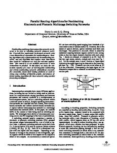
The standard driver discards from further exploration any sequence that results in a state that has already been visited; the driver uses the library method stopIfVisited(Object root) that ignores the current execution path and forces backtracking (to a preceding choice point) if the state reachable from root has already been visited in the exploration. Note that the comparison of states is performed only at the method boundaries (not during method execution), which naturally partitions an execution path into subpaths that each cover execution of one method invocation. As in other related studies [13, 45, 48], we consider a breadth-first exploration of the state space. (A depth-first exploration could miss parts of the state space since state comparison could eliminate a state with a shorter sequence in favor of a state with a longer sequence.) Figure 4 illustrates some states that arise in the state-space exploration corresponding to the call mainStandard(4). Among other states, the exploration visits the five trees of size three shown at the top of the figure. (For simplicity, the figure does not show the BST object that contains size 3 and points to the root node.) The exploration executes add(4) on the five trees of size three. The standard driver separately executes add(4) on each pre-state, resulting in the five post-states shown at the bottom of the figure. The delta driver. Figure 3 also shows a driver that explores states using ∆Execution. The delta driver is similar to the standard driver: both use non-

4

// N bounds sequence length and parameter values public static void mainStandard(int N) { BST bst = new BST(); // empty tree for (int i = 0; i < N; i++) { int methNum = Verify.getInt(0, 1); int value = Verify.getInt(1, N); switch (methNum) { case 0: bst.add(value); break; case 1: bst.remove(value); break; } Standard.stopIfVisited(bst); } }

Figure 2: Driver for standard execution. deterministic choices to select different methods and input values, both prune the exploration based on the state of bst, and both use breadth-first exploration. However, the delta driver differs from the standard driver in the way it operates on the state. First, bst in the delta driver is a ∆State that represents several individual trees. Second, the delta driver backtracks the state differently than the standard driver. Specifically, the method newIteration returns one ∆State containing all individual states that should be explored in a given iteration. In the first iteration, this ∆State is a singleton that has only the initial state (i.e., the empty tree). The method merge at the end of one method execution path collects those trees (from bst) that have not been previously visited and thus should be explored in the next loop iteration. Effectively, the driver combines all distinct states reachable with the method sequences of length i into one ∆State for the iteration i+1. The method newValue updates the internal state for ∆Execution as backtracking should not restore some parts of that internal state (specifically the state mask discussed in Section 3.2). Split and Merge. While standard execution invokes add(4) separately against each standard state, ∆Execution invokes add(4) simultaneously against a set of standard states. ∆Execution itself operates on one state, called a ∆State, which represents a set of individual standard states. We call the operation that combines standard states into a ∆State merging. The top of Figure 4 illustrates one set consisting of the five pre-states. (Section 3.1 describes how to efficiently represent a ∆State, and Section 3.5 describes how to efficiently merge states.) During program execution, ∆Execution occasionally needs to split the ∆State. Informally, we say that a state (or set of states) follows an execution path if ∆Execution operates on that state as it executes that path. For add(4), for example, the five pre-states follow the same execution path until the first check of temp.right == null. At that point, ∆Execution splits the set of states: one subset (of two states) follows the true branch, and the other subset (of three states) follows the false branch. Note that the split enforces the invariant that all states in a set follow the same path. Each split introduces a non-deterministic choice point in the execution. For add(4), one execution with two states terminates after creating a node with value 4 and assigning it to the right of the root. The figure depicts this execution with

5

// N bounds sequence length and parameter values public static void mainDelta(int N) { BST bst = new BST(); // empty tree for (int i = 0; i < N; i++) { bst = Delta.newIteration(bst); int methNum = Verify.getInt(0, 1); int value = Verify.getInt(1, N); Delta.newValue(); switch (methNum) { case 0: bst.add(value); break; case 1: bst.remove(value); break; } Delta.merge(bst); } }

Figure 3: Driver for delta execution. the left arrow. The other execution with three states splits at the second check of temp.right == null: two (middle) states follow the true branch, and one (rightmost) state follows the false branch. These two executions terminate without further splits, appropriately adding the value 4 to the final trees. We next describe the merging that ∆Execution performs to build a ∆State from individual states. Merging is a dual operation of splitting: while splitting partitions a set of states into subsets, merging combines several sets of states (or several individual states) into a larger set. In principle, merging can be performed on any sets of states whenever the executions associated with those states reach the same program point. For example, ∆Execution could merge all three sets of states from Figure 4 when they reach size++. However, our current implementation of ∆Execution considers only the program points that are method boundaries: it merges the states only after all of them finish the execution path for one method, since that is also where state comparison is done. Performance. We next discuss how the performance of ∆Execution and standard execution compare. In our running example, ∆Execution requires only three execution paths to reach all five post-states that add(4) creates for the five pre-states. Additionally, these three paths share some prefixes that can be thus executed only once. In contrast, standard execution requires five executions of add(4), one execution for each pre-state, to reach the five post-states. Also, each of these five separate executions needs to be executed for the entire path. The trade-off between ∆Execution and standard execution can be summarized like this: ∆Execution performs fewer executions (avoiding separate execution of the same path shared by multiple states) than standard execution, but each execution in ∆Execution (that operates on a set of standard states) is more expensive than in standard execution (that operates on one standard state). It is also important to note that the presence of constants (i.e., values that are the same across a set of states) is essential to efficient operations under ∆Execution. Whether ∆Execution is faster or slower than standard execution for some exploration depends on several factors, including the number of execution paths, the number of splits, the cost to execute one path, the number of

6

3

3

3

3

3

3

3

2

1

1

2

1

1

1

3

3

2

2

2

3

add(4) splits on first temp.right == null

splits on second temp.right == null

4

4

4

4

4

3

3

2

1

1

2

4

1

4

1

3

2

1

2

3 4

2

3

4

4

merge

2 1

4

4

4

4

4

3

3

2

1

1

4

1

4

1

3

2

2

3 4

2

4

3 4

Figure 4: Executions of add(4) on a set of states. constants, and the sharing of execution prefixes. The experimental results from Section 5 show that ∆Execution is faster than standard execution for a number of subject programs and values for the bound N from the drivers. For example, for the binary search tree example and N = 10, ∆Execution speeds up JPF 4.41x and our model checker BOX 1.67x, while using over 2x more memory in JPF and 3x more memory in BOX. (On average, ∆Execution uses roughly the same amount of memory as standard execution.)

7

3 33211

??332

211?? ?? 1

??

??

2

?? 2

3

Figure 5: ∆State for the five pre-states from Figure 4.

3

Technique

The key idea of ∆Execution is to execute a program simultaneously on a set of standard states. We first discuss ∆States that represent sets of states. We describe in detail two main operations on ∆States: splitting, which divides a set of states into subsets for executing different program paths, and merging, which combines several states together into a set. We also present how program execution works in ∆Execution and how ∆Execution facilitates an optimized comparison of states.

3.1

∆State

∆Execution represents a set of individual standard states as a single ∆State. Each ∆State encodes all the information from the original individual states. A ∆State includes ∆Objects that can store multiple values (either references or primitives) that exist across the multiple individual states represented by a ∆State. Figures 6, 7, and 8 show the classes used to represent ∆States for the binary search tree example. We discuss here only the field declarations from those classes. (The methods from those classes implement the operations on ∆State and are explained later in the text.) Each object of the class DeltaNode stores a collection of references to Node objects, and each object of the class DeltaInt stores a collection of primitive integer values. The BST and Node objects are changed such that they have fields that are ∆Objects. Figure 5 shows the ∆State that represents the set of five pre-states from Figure 4. Each ∆State consists of layers of “regular” objects and ∆Objects. In this ∆State, each of the pre-states has a corresponding state index that ranges from 0 to 4. Note that we could extract each of the five pre-states by traversing the ∆State while indexing it with the appropriate state index. For example, we can extract the balanced tree using state index 2. Also note that some of the values in the example ∆State are “don’t cares” (labeled with “?”) because 8

the corresponding object is not reachable for that state index. For example, the first node to the left of the root has “?” in the field info for the last two states (with indexes 3 and 4) because those states have the value null for the field root.left. While each ∆Object conceptually represents a collection of values, the implementation does not always need to use collections or arrays. In particular, a value is often constant across all (relevant) states. For example, the info fields for all tree leaves in Figure 5 have constant values (for the relevant states). Our implementation uses an optimized representation for constants. The optimization is straightforward, and we do not discuss it in detail. We point out, however, that the optimization is important both for reducing the memory requirements of ∆States and for improving the efficiency of operations on ∆States.

3.2

Splitting

∆Execution operates on a ∆State that represents a set of standard states. ∆Execution can perform many operations on the entire set. It needs to split the set only at a branch control point (e.g., an if statement) where some states from the set evaluate to different branch outcomes (e.g., for one subset of states, the branch condition evaluates to true, and for the other subset of states, it evaluates to false). We call such points split points; effectively, they introduce non-deterministic choice points as ∆Execution needs to explore both outcomes. (Note that no split is necessary even for branch control points when all states evaluate to the same branch outcome.) One challenge in ∆Execution is to efficiently split ∆States. Our solution is to introduce a state mask that identifies the currently active states within a ∆State. Each state mask is a set of state indexes. At the beginning of an execution, ∆Execution initializes the state mask to the set of all state indexes. For example, the execution of add(4) for the ∆State from Figure 5 starts with the state mask being {0, 1, 2, 3, 4}. At the appropriate branch points, ∆Execution needs to split the set of states into two subsets. Our approach does not explicitly divide a ∆State into two ∆States; instead, it simply changes the state mask to reflect the splitting of the set of states. Specifically, ∆Execution builds a new state mask to identify the new subset of active states in the ∆State. It also saves the state mask for the other subset that should be explored later on. The execution then proceeds with the new subset. After ∆Execution finishes the execution path for some (sub)set of states, it backtracks to some unexplored split point to explore the other path using the state mask saved at the split point. Backtracking changes the state mask but restores the ∆State to exactly what it was at the split point. Backtracking can be implemented in several ways; Section 4 discusses how JPF uses state saving and restoration while BOX uses re-execution. To illustrate how the state mask changes during the execution, consider the example from Figure 4. The state mask is initially {0, 1, 2, 3, 4}. At the first split point, the execution proceeds with the state mask being {0, 1}. After the 9

first backtracking, the state mask is set to {2, 3, 4}. At the second split point, the execution proceeds with the state mask being {2, 3}. After the second backtracking, the state mask is set to {4} for the final execution. Appropriate use of a state mask can facilitate optimizations on the ∆State. Consider, for example, a ∆Object that is not a constant when all states are active. This object can temporarily be transformed into a constant if all its values are the same for some state mask occurring during the execution. For instance, in our running example, the value of root.right becomes the constant null when the state mask is {0, 1}. Additionally, the state mask allows the use of sparse representations for ∆Objects: instead of using an array to map all possible state indexes into values, a sparse ∆Object can use representations that map only the active state indexes into values, thereby reducing the memory requirement.

3.3

Program execution model

We next discuss how ∆Execution executes program operations. The key is to execute each operation simultaneously on a set of values. ∆Execution uses a non-standard program execution that manipulates a ∆State that represents a set of standard states. Such non-standard execution can be implemented in two ways: (1) instrumenting the code such that the regular execution of the instrumented code corresponds to the non-standard execution [26, 43, 48] or (2) changing the execution engine such that it interprets the operations in the non-standard semantics [13]. Our current implementation uses instrumentation: the subject code is preprocessed to support ∆Execution. We use parts of the instrumentation to describe the semantics of ∆Execution. 3.3.1

Classes

The instrumentation changes the original program classes and generates new classes for ∆Objects. Figure 1 from Section 2 shows a part of the original code for the binary search tree example. Figures 6, 7, and 8 show the key parts of the instrumented code for this example. Figure 6 shows the instrumented version of the original BST and Node classes. Figure 7 shows the new class DeltaNode that stores and manipulates the multiple Node references that can exist across the multiple states in a ∆State. Figure 8 shows the class DeltaInt that stores and manipulates multiple int values; this class is a part of the ∆Execution library and is not generated anew for each program. It is important to note that ∆Objects are immutable from the perspective of the instrumented code in the same way that regular primitive and reference values are immutable for standard execution. This allows sharing of ∆Objects. For example, this allows direct assignment of one DeltaInt object to another (e.g., int x = y simply becomes DeltaInt x = y). Our implementation internally mutates ∆Objects to achieve higher performance, in particular when values become constant across active states. The mutation handles the situations that involve shared ∆Objects and require a “copy-on-write” cloning.

10

public class BST { private DeltaNode root = DeltaNode.NULL; private DeltaInt size = DeltaInt._new(0); public void add(DeltaInt info) { if (get_root().eq(DeltaNode.NULL)) set_root(DeltaNode._new(info)); else for (DeltaNode temp = get_root(); true; ) if (temp.get_info().lt(info)) { if (temp.get_right().eq(DeltaNode.NULL)) { temp.set_right(DeltaNode._new(info)); break; } else temp = temp.get_right(); } else if (temp.get_info().gt(info)) { if (temp.get_left().eq(DeltaNode.NULL) { temp.set_left(DeltaNode._new(info)); break; } else temp = temp.get_left(); } else return; // no duplicates } set_size(get_size().add(DeltaInt._new(1))); } public DeltaBoolean remove(DeltaInt info) { ... } } class Node { DeltaNode left, right; DeltaInt info; Node(DeltaInt info) { this.info = info; } }

Figure 6: Instrumented BST and Node classes. 3.3.2

Types

The instrumentation changes all types in the original program to their delta versions. Comparing figures 1 and 6, notice that the occurrences of Node and int have been replaced with the new DeltaNode class (from Figure 7) and the DeltaInt class (from Figure 8), respectively. The instrumentation also appropriately changes all definitions and uses of fields, variables, and method parameters to use ∆Objects. 3.3.3

Field accesses

The instrumentation replaces standard object field reads and writes with calls to new methods that read and write fields across multiple objects. For example, all reads and writes of Node fields are replaced with calls to getter and setter methods in DeltaNode. Consider, for instance, the field read temp.left. In ∆Execution, temp is no longer a reference to a single Node object but a reference to a DeltaNode object that tracks multiple references to possibly many different Node objects. The left field of Node is now accessed via the get left method in DeltaNode. This method returns a DeltaNode object that references (one or more) Node objects that correspond to the left fields of all temp objects whose states are active in the state mask. In general, this can result in an execution split when some objects in temp are null. 11

class DeltaNode { // maps each state index to a Node object Node[] values; // conceptually DeltaNode(int size) { values = new Node[size]; } private DeltaNode(Node n) { values = new Node[]{ n }; } public static DeltaNode _new(DeltaInt info) { return new DeltaNode(new Node(info)); } public boolean eq(DeltaNode arg) { StateMask sm = StateMask.getStateMask(); StateMask trueMask = new StateMask(sm.size()); StateMask falseMask = new StateMask(sm.size()); foreach (int index : sm) if (values[index] == arg.values[index]) trueMask.enable(index); else falseMask.enable(index); boolean result; if (trueMask.isEmpty()) result = false; else if (falseMask.isEmpty()) result = true; else result = (Verify.getInt(0, 1) == 0); // split StateMask.setStateMask(result ? trueMask : falseMask); return result; } public DeltaNode get_left() { StateMask sm = StateMask.getStateMask(); DeltaNode result = new DeltaNode(sm.size()); foreach (int index : sm) { DeltaNode dn = values[index].left; result.values[index] = dn.values[index]; } return result; } public void set_left(DeltaNode arg) { StateMask sm = StateMask.getStateMask(); IdentitySet set = new IdentitySet(); foreach (int index : sm) { Node n = values[index]; if (set.add(n)) // true if n was added n.left = n.left.clone(); n.left.values[index] = arg.values[index]; } } public DeltaNode get_right() { ... } public void set_right(DeltaNode arg) { ... } public DeltaInt get_info() { ... } public void set_info(DeltaInt arg) { ... } }

Figure 7: New DeltaNode class. 3.3.4

Operations

The instrumentation replaces (relational and arithmetic) operations on reference and primitive values with method calls to DeltaNode and DeltaInt objects. All original operations on values now operate on ∆Objects that represent sets of values. More precisely, the methods in ∆Objects do not need to operate on all values but only on those values that correspond to the active state indexes as indicated by the state mask. For an example arithmetic operation, consider integer addition. In standard 12

class DeltaInt { // maps each state index to an integer value int[] values; // conceptually DeltaInt add(DeltaInt arg) { StateMask sm = StateMask.getStateMask(); DeltaInt result = new DeltaInt(sm.size()); foreach (int index : sm) result.values[index] = values[index] + arg.values[index]; return result; } ... }

Figure 8: Part of DeltaInt library class. execution, the addition takes two integer values and creates a single value. In ∆Execution, it takes two DeltaInt objects and creates a new DeltaInt object. The add method in DeltaInt (From Figure 8) shows how ∆Execution conceptually performs pairwise addition across all active state indexes for the two DeltaInt objects. Our implementation optimizes the cases when those objects are constant (to avoid the loop or state indexing). For an example relational operation, consider reference equality. The method eq in DeltaNode (from Figure 7) performs this operation across all active state indexes. Note that this method can create a split point in the execution if the result of the operation differs across the states. If so, eq introduces a nondeterministic choice (with getInt) that returns a boolean true or false after appropriately setting the state mask. 3.3.5

Method calls

The instrumentation replaces a standard method call with a method call whose receiver is a ∆Object, which allows making the call on several objects at once. Note that each call introduces a semantic branch point (since different objects may have different dynamic types) and can result in an execution split.

3.4

Optimized state comparison

Heap symmetry [9,23,28,30] is an important technique that model checkers use to alleviate the state-space explosion problem. Heap symmetry detects equivalent states: when the exploration encounters a state equivalent to some already visited, the exploration path can be pruned. In object-oriented programs, two heaps are equivalent if they are isomorphic (i.e., have the same structure and primitive values, while their object identities can vary) [6, 23, 30]. An efficient way to compare states for isomorphism is to use linearization (also known as serialization or marshalling) that translates a heap into a sequence of integers such that two heaps are isomorphic if and only if their linearizations are equal. ∆Execution exploits the fact that different heaps in a ∆State can share prefixes of linearization. Instead of computing linearizations separately for each state in a set of states, ∆Execution simultaneously computes a set of lineariza-

13

void linearize(Object o, StateMask sm) { foreach (int index : sm) { Pair(Map _, Seq s) = linObject(o, new Map(), index); checkVisited(index, s); } } Pair linObject(Object o, Map ids, int index) { if (o == null) return Pair(ids, Seq(NULL)); if (o in ids) return Pair(ids, Seq(ids.get(o))); int id = ids.size(); return linFields(o, ids.put(o, id), Seq(id), index); /*return linFields(o, 0, ids.put(o, id), Seq(id), index);*/ } Pair linFields(Object o, Map ids, Seq seq, int index) { for (int f = 0; f < o.numberOfFields(); f++) { Object fo = o.getField(f).values[index]; Pair(ids, Seq s) = linObject(fo, ids, index); seq = seq.append(s); } return Pair(ids, seq); } Pair linFields(Object o, int f, Map ids, Seq seq, int index) { if (f < o.numberOfFields()) { Object fo = o.getField(f).values[index]; Pair(Map m, Seq s) = linObject(fo, ids, index); return linFields(o, f + 1, m, seq.append(s), index); } else return Pair(ids, seq); }

Figure 9: Non-optimized linearization of ∆State. tions for a ∆State. Sharing the computation for the prefixes not only reduces the execution time but also reduces memory requirements as it enables sharing among the sequences used for linearizations. We next present how to transform a basic algorithm that separately linearizes each state from a ∆State into an efficient algorithm that simultaneously linearizes all states from a ∆State. Figure 9 shows a pseudo-code of a basic algorithm that iterates over each active state from the state mask and computes the linearization for the individual state. For simplicity of presentation, this algorithm assumes that the heaps contain only reference fields of only one class. Our actual implementation handles general heaps with objects of different classes, primitive fields, and arrays. The method linObject produces a sequence of integers that represent linearization for the state reachable from o. When o is null, linObject returns a singleton sequence with the value that represents null. When o is a reference to a previously linearized object, linObject returns a singleton sequence with the identifier used for that object, which handles object aliasing. The map ids stores the association between objects and their ids. When o is an object not yet linearized, linObject creates a new id for it, appropriately extends the map, and linearizes all the object fields. The method linFields linearizes the fields of a given object. A typical

14

Stack stack; // mutable structure void linearize(Object o, StateMask sm) { stack = new Stack(); Triple(Map _, Seq s, StateMask tm) = linObject(o, new Map(), sm); checkVisited(tm, s); // all states from tm have sequence s while (!stack.isEmpty()) { Tuple(Object o, int f, Map ids, Seq seq, StateMask nm) = stack.pop(); Triple(Map _, Seq s, StateMask tm) = linFields(o, f, ids, seq, nm); checkVisited(tm, s); } } Triple linObject(Object o, Map ids, StateMask sm) { if (o == null) return Triple(ids, Seq(NULL), sm); if (o in ids) return Triple(ids, Seq(ids.get(o)), sm); int id = ids.size(); return linFields(o, 0, ids.put(o, id), Seq(id), sm); } Triple linFields(Object o, int f, Map ids, Seq seq, StateMask sm) { if (f < o.numberOfFields()) { Triple(Object fo, StateMask em, StateMask nm) = split(o.getField(f), sm); if (nm is not empty) stack.push(o, f, ids, seq, nm); Triple(StateMask om, Map m, Seq s) = linObject(fo, ids, em); return linFields(o, f + 1, m, seq.append(s), om); } else return Triple(sm, ids, seq); }

Figure 10: Optimized linearization of ∆State. implementation is iterative, as shown in the first linFields method. It is important to note that the value of the expression o.getField(f).values[index] determines the linearizations for different states. We target this expression to be the split point in our optimized linearization algorithm. The algorithm thus needs to explore different execution paths from this point, effectively performing backtracking. We want to implement the optimized algorithm to execute on a regular JVM, so to support backtracking. An intermediate step in the optimization is to transform the algorithm to conceptually use the continuation-passing style [19]. In practice, the method linFields is transformed into a recursive implementation shown in the second linFields method. This version exposes the field index f and linearizes the fields of o between f and o.getNumberOfFields(). This version permits the linearization to continue an execution from the point it was left at in linFields. Note that linFields and linObject manipulate functional objects Map and Seq, which facilitates backtracking of the state. Figure 10 shows the pseudo-code of the optimized algorithm that linearizes a ∆State in the ∆Execution mode. The new methods linObject and linFields do not take one state index but a state mask with several active state indexes to linearize. These methods now return a state mask and one linearization for all 15

the states in that state mask. The linearization can introduce non-deterministic choices to enforce the invariant that all states in the state mask have the same linearization prefix. When the linearization completes for some state mask, it needs to backtrack to explore the remaining state masks. The stack object stores the backtracking points. Each entry stores the state that needs to be restored to continue an execution from a split point: the root object, the field index, the map for object identifiers, the current linearization sequence, and the state mask. While stack is mutable, the other structures are immutable, which makes it easy to restore the state. The while loop in linearize visits each pending backtracking point until it finishes computing all linearizations. The only source of non-determinism in the linearization is the reading of fields across different states from the state mask. The method split takes as input a ∆Object do = o.getField(f) and a state mask sm. It returns a standard object fo = do.values[idx] for some idx from sm, a state mask em of index values such that do.values[index] == fo, and a state mask nm of index values such that do.values[index] != fo. At this point, linFields first pushes on the stack an entry with the backtracking information for nm and then continues the linearization of fo for the states in em.

3.5

Merging

The dual of splitting sets of states into subsets is merging several sets of states into a larger set. Recall the driver for ∆Execution from Figure 3. It merges all non-visited states from one iteration into a ∆State to be used at the start of the next iteration. Specifically, the merge method receives as the input a ∆State and (implicitly) a state mask. This method extracts the non-visited states from the ∆State and only stores their linearized representations. The method newIteration builds and returns a new ∆State from the stored linearized representations. Our merging uses delinearization to construct a ∆State from the linearized representations of non-visited states. The standard delinearization is an inverse of linearization: given one linearized representation, delinearization builds one heap isomorphic to the heap that was originally linearized. The novelty of our merging is that it operates on a set of linearized representations simultaneously and, instead of building a set of standard heaps, it builds one ∆State that encodes all the heaps. It is interesting to point out that we often used in debugging our implementation the fact that linearization and delinearization are inverses; the composition of these functions gives the identity function: for any set of linearizations s, the linearization of the delinearization of s should equal s. We highlight two important aspects of the merging algorithm. First, it identifies ∆Objects that should be constants (with respect to the reachability of the nodes), which results in a more efficient ∆State. Such constants can occur quite often; for instance, in our experiments (see Section 5), the lowest percentage of the constant ∆Objects in the merged ∆States is 33%. Second, the merging al16

gorithm greedily shares the objects in the resulting ∆State: it attempts to share the same ∆Object among as many individual states as possible. For example, in Figure 5, the left node from the root is shared among three of the five states. Figure 11 shows the pseudo-code of our merging algorithm. The input is a collection of linearizations, and the output is a root object for a ∆State. The algorithm maintains a collection of maps from object ids to actual objects (which handles aliasing) and a collection of offsets that track progress through the different linearizations (since they do not need to go in a “lockstep”). The method createObject constructs one object shared for all states in the given state mask and invokes createDeltaObject to construct each field of the object. Note that this sharing does not constitute aliasing in the standard semantics since: only one reference is visible for any given state. The method createDeltaObject examines the field values across all states in the state mask sm. For each state it checks for three possible options for the field’s object id: (1) it denotes the null reference, (2) it denotes an alias, or (3) it denotes a new object. For the first two options the algorithm assigns the value to the delta object d as it performs the check. For the third it just records in the state mask object cm the index of the state during the check. If the statemask cm is not empty after the check across all states, the algorithm recursively invokes (once) createObject to create an object that will be shared among the states in cm. Lastly, the algorithm checks if the the delta object d is semantically a constants, i.e., it contains the same value across all states denoted by sm. A special constant object is created in that case. For states that have aliases between objects (unlike binary search tree), this greedy algorithm does not always produce a ∆State with the smallest number of nodes, and some alternative algorithms could produce smaller graphs. Figure 12 illustrates an example where an alternative merging algorithm could find more sharing. Given the two states at the top, our greedy algorithm produces the ∆State at the bottom-left that does not share the two subgraphs denoted by shaded triangles. In contrast, a more complex algorithm could potentially identify this sharing opportunity and construct the ∆State at the bottom-right. However, such alternative algorithms would require more time to search for appropriate sharing opportunities that result in smaller ∆States.

4

Implementation

We have implemented ∆Execution in two model checkers, JPF and BOX. JPF [42] is a popular model checker for Java programs, but it is general-purpose and has a high overhead [14] for the subject programs considered in our study and related studies [14,44,45]. We have thus implemented a specialized model checker, called BOX (from Bounded Object eXploration), for efficient exploration of such subject programs.

17

Seq[] lin; // input Map[] maps; // intermediate result, mutable int[] offsets; // intermediate result, mutable Object merge() { maps = new Map[lin.length](); // all empty maps offsets = new int[lin.length]; // all zeroes // the state mask starts as the set {0..lin.length-1} return createObject(new StateMask(lin.length)); } Object createObject(StateMask sm) { Object o = new Object(); foreach (int index : sm) { int id = lin[index][offsets[index]++]; maps[index].put(id, o); } foreach (field f in o) o.f = createDeltaObject(sm); return o; } DeltaObject createDeltaObject(StateMask sm) { DeltaObject d = new DeltaObject(lin.length); // state indexes for which to create a new object StateMask cm = new StateMask(); foreach (int index : sm) { int id = lin[index][offsets[index]++]; if (id == NULL) d.values[index] = null; else if (maps[index].contains(id)) d.values[index] = maps[index].get(id); else { // need to create a new object for this id cm.add(index); offsets[index]--; } } if (cm not empty) { // key: greedily sharing the new object across indexes Object co = createObject(cm); foreach (int index : cm) d.values[index] = co; } // optimization for constants if (d.values is constant with respect to sm) d = new DeltaObjectConstant(d.values[some index from sm]); return d; }

Figure 11: Pseudo-code of the merging algorithm.

4.1

JPF

We have implemented ∆Execution by modifying JPF version 4 [1]. JPF is implemented as a backtrackable Java Virtual Machine (JVM) running on top of a regular, host JVM. JPF provides operations for state-space exploration: storing states, restoring them during backtracking, and comparing them. By default, JPF compares the entire JVM state that consists of the heap, stack (for each thread), and class-info area (that is mostly static but can be modified due to the dynamic class loading in Java). However, our experiments require only the part of the heap reachable from the root object in the driver. We have therefore disabled the JPF’s default state comparison and instead use a specialized state comparison as done in some previous studies with JPF [13, 45, 48]. We next discuss how we have implemented each component of ∆Execution in JPF. We call the resulting system ∆JPF. ∆JPF keeps ∆State as a part of the JPF state, which enables the use of JPF backtracking to restore ∆State at the split points. We have implemented the library operations on ∆State (such as 18

1111 0000 0000 1111 0000 1111 0000 1111 0000 1111 0000 1111

Greedy

111 000 000 111 000 111 000 111 000 111 000 111

Alternative

?

0000 1111 1111 0000 0000 1111 0000 1111 0000 1111

0000 1111 1111 0000 0000 1111 0000 1111 0000 1111

000 111 111 000 000 111 000 111 000 111

Figure 12: Greedy vs. alternative merging. arithmetic and relational operations or field reads and writes) to execute on the host JVM. Effectively, the library forms an extension of JPF; our goal is not to model check the library itself but the subject code that uses the library. ∆JPF uses instrumented code to invoke the operations that manipulate the ∆State. We have implemented splitting in ∆JPF on top of the existing non-deterministic choices in JPF. It is important to point out that our implementation leverages JPF to restore the entire ∆State but uses state masks to indicate the active states. Therefore, ∆JPF manages state masks on the host JVM, outside of the backtracked state. We have implemented merging also to execute on the host JVM and to create one ∆State as a JPF state that encodes all the nonvisited states encountered in the previous iteration of the exploration. Recall from Section 2 that the drivers in our experiments use breadth-first exploration. ∆JPF does not use the optimized state comparison (Section 3.4) except for the non-exhaustive exploration as described in Section 5.3. To automate the instrumentation of code for execution on ∆JPF, we have developed a plug-in for Eclipse version 3.2 [17]. This plug-in takes a subject program and manipulates its Eclipse internal AST representation to automate the steps described in Section 3.3.

4.2

BOX

We have developed BOX, a model checker optimized for sequential Java programs. JPF is a general-purpose model checker for Java that can handle concurrent code and can store/restore/compare the entire JVM state that consists of heap, stack, and class-info area. However, in unit testing of object-oriented programs, most code is sequential and most drivers need to store/restore/compare only the heap part of the state. Therefore, we have used the existing ideas from state-space exploration research [2, 10, 18, 20, 23, 31, 36, 42] to engineer a 19

high-performance model checker for such cases. BOX can store/restore/compare only a part of the program heap reachable from a given root. The root corresponds to the main object under exploration in the driver. BOX uses a stateful exploration (by restoring the entire state) across iterations and stateless exploration (by re-executing one method at a time) within one iteration. BOX needs to re-execute a method within an iteration as it does not store the state of the program stack. Instead, BOX only keeps a list of changes performed on the heap during a single method execution and restores the state by undoing those changes. For efficient manipulation of the changes, BOX requires that code under exploration be instrumented. We refer to the ∆Execution implementation in BOX as ∆BOX. ∆BOX needs to backtrack the ∆State in order to explore a method for various state masks. ∆BOX re-executes the method from the beginning to reach the latest split point. While re-execution is seemingly slow, it can actually work extremely well in many situations. For example, Verisoft [20] is a well-known model checker that effectively employs re-execution. ∆BOX implements the components of ∆Execution as presented in Section 3. ∆BOX represents ∆State as a regular Java state that contains both ∆Objects and objects of the instrumented classes. Our instrumentation for ∆BOX (as well as for BOX) is mostly manual at this time. ∆BOX uses instrumented code to perform the operations on the ∆State. Similarly to ∆JPF, ∆BOX merges states between iterations of the breadth-first exploration. ∆BOX always employs the optimized state comparison as presented in Section 3.4.

5

Evaluation

We present an experimental evaluation of ∆Execution. We first describe the ten basic subject programs used in the evaluation and then discuss the improvements that ∆Execution provides for an exhaustive exploration of these programs in both JPF and BOX and a non-exhaustive exploration in JPF. We finally present the improvements that ∆Execution provides on a larger case study, an implementation of the AODV routing protocol [34]. We performed all experiments on a Pentium 4 3.4GHz workstation running under RedHat Enterprise Linux 4. We used Sun’s JVM 1.5.0 07, limiting each run to 1.8GB of memory and 1 hour of elapsed time.

5.1

Basic subjects

We evaluated ∆Execution on ten subject programs taken from a variety of sources. All but one of these subjects have been previously used to evaluate testing and model-checking techniques. The following nine subjects are data structures: • binheap is an implementation of priority queues using binomial heaps [45]

20

• bst is our running example that implements a set using binary search trees [6, 48] • deque is our implementation of a double-ended queue using doubly-linked lists • fibheap is an implementation of priority queues using Fibonacci heaps [45] • heaparray is an array-based implementation of priority queues [6, 48] • queue is an object queue implemented using two stacks [15] • stack is an object stack [15] • treemap is an implementation of maps using red-black trees based on Java collection 1.4 [6, 45, 48] • ubstack is an array-based implementation of a stack bounded in size, storing integers without repetition [11, 33, 40, 47] The tenth subject is filesystem, which is based on the Daisy file-system code [35]. While the original code had seeded errors, we use a corrected version from another study [15]. The primary purpose of our evaluation is to compare the efficiency of ∆Execution and standard execution, so we use correct implementations of all basic subjects. (The AODV case study described in Section 5.4 uses code with errors that violate a safety property.) For each subject, we wrote drivers for standard execution and for ∆Execution (similar to figures 2 and 3). The drivers exercise the main mutator methods. For data structures, the drivers add and remove elements. For filesystem, the drivers create and remove directories, create and remove files, and write to and read from files.

5.2

Exhaustive exploration

Figure 13 shows the experimental results for exhaustive exploration. For each subject and several bounds (on the sequence length and parameter size, as in the driver shown in Figure 3), we tabulate the overall exploration time and peak memory usage with and without ∆Execution in both JPF and BOX, and the characteristics of the explored state spaces. The cells marked with “*” represent that the experiment either ran out of 1.8GB memory or exceeded the 1 hour time limit. The columns labeled “std/delta” show the improvements that ∆Execution provides over standard execution. Note that the numbers are ratios and not percentages; for example, for binheap and N = 7, the ratio is 9.55x, which corresponds to about 90% improvement. For JPF, the speedup ranges from 1.03x (for filesystem and N = 3) to 100.81x (for heaparray and N = 9), with the average of 10.97x, which is over an order of magnitude improvement. (The averages are geometric means over all the experiments.) For BOX, the speedup ranges from 0.58x (for filesystem and N = 3) to 4.27x (for stack and N = 7), with the average of 2.07x. 21

22

experiment subject N 7 binheap 8 9 9 bst 10 11 8 deque 9 10 6 fibheap 7 8 3 filesystem 4 5 8 heaparray 9 10 6 queue 7 8 6 stack 7 8 10 treemap 11 12 8 ubstack 9 10 gmean -

std 25.40 466.00 * 44.34 216.72 * 54.86 550.57 * 3.13 24.88 398.13 2.03 17.13 * 104.50 2,718.12 * 7.76 104.41 * 4.95 59.44 * 579.50 1,754.34 * 60.37 1,482.75 * -

JPF time delta std/delta 2.66 9.55x 15.34 30.37x * * 10.98 4.04x 49.17 4.41x * * 6.64 8.27x 57.72 9.54x * * 1.52 2.06x 3.13 7.94x 28.31 14.06x 1.98 1.03x 3.70 4.63x * * 4.18 24.99x 26.96 100.81x * * 1.62 4.79x 6.37 16.38x * * 1.46 3.38x 5.08 11.71x * * 7.61 76.14x 19.42 90.34x * * 6.26 9.64x 48.75 30.41x * * 10.97x

JPF mem. std/delta 1.16x 1.03x * 0.70x 0.46x * 1.50x 1.48x * 0.98x 2.13x 0.88x 0.97x 11.50x * 2.31x 1.22x * 2.64x 1.77x * 1.01x 1.31x * 2.69x 3.04x * 1.57x 1.48x * 1.51x

std 0.80 11.70 107.14 2.45 12.65 68.31 2.30 22.53 280.66 0.22 1.17 16.89 0.15 1.20 37.84 1.24 12.02 128.27 0.37 3.90 78.79 0.31 2.93 60.07 3.29 10.80 32.81 2.28 22.69 271.56 -

BOX time delta std/delta 0.35 2.26x 3.40 3.44x 32.91 3.26x 1.55 1.58x 7.57 1.67x 49.86 1.37x 0.83 2.77x 7.58 2.97x 100.22 2.80x 0.16 1.34x 0.67 1.75x 9.80 1.72x 0.25 0.58x 0.72 1.67x 30.01 1.26x 0.89 1.39x 9.00 1.33x 110.78 1.16x 0.18 2.10x 0.94 4.14x 25.32 3.11x 0.12 2.50x 0.68 4.27x 17.80 3.37x 1.25 2.63x 3.26 3.32x 9.14 3.59x 1.29 1.77x 13.59 1.67x 175.61 1.55x 2.07x

BOX mem. std/delta 2.71x 1.08x 1.04x 0.77x 0.30x 0.18x 1.54x 1.14x 1.18x 1.24x 0.68x 1.72x 0.97x 1.24x 0.53x 0.58x 1.44x 1.00x 1.87x 1.31x 1.04x 1.38x 1.34x 1.30x 0.66x 0.62x 0.97x

# states 16864 250083 1353196 46960 206395 915641 69281 623530 6235301 3003 36730 544659 58 1353 64576 97092 804809 8722946 10057 147995 2578641 9331 137257 2396745 13076 35405 96401 109681 991189 9922641 -

# executions std delta std/delta 236096 401 588 4001328 863 4636 24357528 1069 22785 845280 10846 77 4127900 22688 181 20144102 46731 431 1108496 576 1924 11223540 810 13856 124706020 1100 113369 21021 82 256 293840 130 2260 4901931 209 23454 6264 576 10 194832 1568 124 11623680 3940 2950 873828 258 3386 8048090 359 22418 95952406 488 196623 70399 45 1564 1183960 60 19732 23207769 77 301399 65317 42 1555 1098056 56 19608 21570705 72 299593 261520 3579 73 778910 5269 147 2313624 7774 297 987129 595 1659 9911890 931 10646 109149051 1414 77191 3040x

Figure 13: Overall time and memory for exhaustive exploration in JPF and BOX and characteristics of the explored state spaces.

experiment

standard execution time

∆Execution time

subject

N

exec.

comp.

backt.

exec.

comp.

backt.

merg.

binheap

7 8 9 10 6 7 8 10 11

18.21 369.49 20.77 104.54 1.24 15.03 257.91 567.16 1,724.36

0.54 5.55 3.75 20.68 0.07 0.52 8.21 2.65 8.55

6.65 90.97 19.81 91.50 1.82 9.33 132.01 9.69 21.44

0.57 4.09 2.30 7.32 0.21 0.40 3.89 1.39 2.48

0.59 6.11 5.42 31.98 0.13 0.79 11.43 4.34 14.36

1.10 1.04 2.01 4.02 1.06 1.09 1.34 1.48 1.59

0.39 4.10 1.26 5.86 0.12 0.84 11.64 0.41 0.98

bst

fibheap treemap

Figure 14: Time breakdown for JPF experiments. Note that the ratio less than 1.00 means that ∆Execution ran slower (or required more memory) than standard execution, for example for filesystem and N = 3 in BOX. While this can happen for smaller bounds, ∆Execution consistently runs faster than standard execution for important cases with larger bounds. ∆Execution provides these significant improvements because it exploits the overlap among executions in the state-space exploration. Figure 13 shows the information about the state spaces explored in the experiments. Note that the number of explored states is the same with and without ∆Execution. This is as expected: ∆Execution focuses on improving the exploration time and does not change the exploration itself. (We used the difference in the number of states to debug our implementations of ∆Execution.) However, the numbers of executions with and without ∆Execution do differ, and the column labeled “std/delta” shows the ratio of the numbers of executions. The ratio ranges from 10x to 301399x. While this ratio effectively enables ∆Execution to provide the speedup, there is no strict correlation between the ratio and the speedup. The overall exploration time depends on several factors, including the number of execution paths, the number of splits, the cost to execute one path, the frequency of constants in ∆States, and the sharing of execution prefixes. 5.2.1

Time

We next discuss in more detail where state-space exploration spends time and where ∆Execution reduces the time. Each state-space exploration includes three components—(1) code execution, (2) state comparison, and (3) state backtracking—and ∆Execution additionally includes (4) merging. Figures 14 and 15 show the breakdown of the overall exploration time on these four components for JPF and BOX. We show the numbers for only some of the experiments (for subjects from Section 5.3); the conclusions are the same for the other experiments. In JPF, ∆Execution significantly reduces the time for code execution and state backtracking. For example, for binheap and N = 7, ∆Execution reduces the execution time from 18.21s to 0.57s and the backtracking time from 6.65s to 1.10s. These savings are big enough and make the times for merging and state comparison irrelevant. (For this exploration, ∆JPF does not even use the 23

experiment subject

binheap

bst

fibheap

treemap

standard execution time

∆Execution time

N

exec.

comp.

backt.

exec.

comp.

backt.

merg.

7 8 9 9 10 11 6 7 8 10 11 12

0.23 4.58 21.64 0.17 0.60 3.05 0.06 0.32 4.77 0.20 0.60 1.51

0.34 3.72 68.57 1.93 10.72 57.79 0.08 0.54 7.80 2.86 9.72 29.69

0.14 2.88 15.27 0.19 0.97 4.71 0.04 0.24 3.90 0.20 0.52 1.26

0.09 1.03 4.73 0.48 1.83 8.16 0.04 0.20 2.79 0.34 0.64 1.47

0.15 1.45 21.95 0.74 3.83 20.46 0.05 0.24 3.78 0.78 2.29 6.91

0.00 0.01 0.00 0.01 0.01 0.02 0.00 0.00 0.00 0.01 0.02 0.02

0.06 0.87 6.20 0.28 1.85 21.06 0.02 0.18 3.15 0.07 0.23 0.67

Figure 15: Time breakdown for BOX experiments. optimized state comparison, from section 3.4.) As mentioned earlier, JPF is a general-purpose model checker that stores and restores the entire Java states and thus has a high execution and backtracking overhead. In BOX, ∆Execution sometimes results in a higher code execution time, yet has a smaller overall exploration time. The reason is that ∆Execution achieves significant savings in the state comparison using the optimized algorithm from Section 3.4. For example, for bst and N = 11, ∆Execution increases the execution time from 3.05s to 8.16s. However, it reduces the state comparison time from 57.79s to 20.46s, which more than makes up for the longer execution time. Note that the number of states and state comparisons is the same in both standard execution and ∆Execution, but the optimized state comparison is only possible for ∆Execution. Indeed, it is the execution on ∆States that enables the simultaneous comparison of a set of states. 5.2.2

Memory

Figure 13 also provides a comparison of memory usage. Specifically, the columns labeled “mem. std/delta” show the ratio of peak memory usage for standard execution versus ∆Execution. Our setup uses the Sun’s jstat monitoring tool to record the peak usage of garbage-collected heap in the JVM running an experiment. Although this particular measurement does not include the entire memory used by the JVM process, it does represent the most relevant amount used by a model checker. (The cells marked “-” represent experiments where the running time is so short that jstat does not provide accurate memory usage.) For JPF, standard execution uses more memory than ∆Execution for most experiments and uses 1.51x more memory on average. However, ∆Execution occasionally uses more memory, for example for bst. For BOX, ∆Execution and standard execution on average use about the same amount of memory. Many factors, already mentioned for exploration time, can influence the memory usage, but an important factor seems to be the number of constant ∆Objects. ∆Execution uses these objects to represent values that are the same across all states in a ∆State. There is a relatively strong positive correlation between the percentage of constant ∆Objects and the memory ratio for an 24

experiment subject N binheap 28 binheap 29 binheap 30 bst 20 bst 21 bst 22 fibheap 28 fibheap 29 fibheap 30 treemap 20 treemap 21 treemap 22 gmean -

standard execution #states #exec. tot.time 28 15680 4.38 29 16820 4.49 30 18000 4.64 166064 10168360 546.65 381535 22466178 1,232.00 677848 43605496 2,397.16 881 182323 18.73 961 184320 18.94 1144 289571 28.53 11879 1492080 808.72 22455 2893212 1,478.80 38126 4918100 2,275.67 -

#states 28 29 30 150192 416946 626555 1041 1157 1354 11952 20590 36550 -

∆Execution #exec. tot.time 956 4.12 958 4.12 1040 4.22 49645 88.70 77951 228.19 83569 367.64 7810 20.25 7269 20.19 10981 28.15 39131 43.50 48974 67.80 59693 105.00 -

ratio tot. impr. 1.06x 1.09x 1.10x 6.16x 5.40x 6.52x 0.93x 0.94x 1.01x 18.59x 21.81x 21.67x 3.37x

Figure 16: Overall time for non-exhaustive exploration. experiment. For example, bst and N = 11 has a poor memory ratio, and the percentage of constant objects in ∆States is 33%, the lowest of all subjects. For treemap and N = 12, on the other hand, ∆Execution uses less memory than standard execution, and the percentage of constant objects is 69%. These percentages are computed across the entire exploration: it is the percentage of constant delta objects produced during merging from the total number of delta objects produced. The Ph.D. dissertation of the first author [12] includes more details on the impact of constants on memory and time performance.

5.3

Non-exhaustive exploration

We next evaluate ∆Execution for a different state-space exploration. While exhaustive exploration is the most commonly used, there are several others such as random [11, 33] or symbolic execution [13, 26, 48]. Recently, Visser et al. [45] have proposed abstract matching, a technique for non-exhaustive statespace exploration of data structures. The main idea of abstract matching is to compare states based on their shape abstraction: two states that have the same shape are considered equivalent even if they have different values in nodes. For example, all binary search trees of size one are considered equivalent. The exploration is pruned whenever it reaches a state equivalent to some previously explored state, which means that abstract matching can miss some portions of the state space. We have chosen to evaluate ∆Execution for abstract matching because the JPF experiments done by Visser et al. [45] have shown that abstract matching achieves better code coverage than five other exploration techniques, including exhaustive exploration, random, and symbolic execution. (The experiments did not consider whether higher code coverage results in finding more bugs.) Our evaluation uses the same four subjects used to evaluate abstract matching in JPF: binheap, bst, fibheap, and treemap. We ran each subject for sequence bound up to N = 30 (as done in [45]) or until the experiment timed out of 1 hour. We used the same drivers as for exhaustive exploration but randomized

25

the order of non-deterministic choices in getInt and used 10 different random seeds; Visser et al. use the same experimental setup to minimize the bias that a fixed order of method/value choices could have when combined with abstract matching. Figure 16 shows the results for abstract matching with and without ∆Execution. ∆Execution significantly reduces the overall exploration time for two subjects (bst and treemap) and slightly reduces or increases the time for the other two subjects (binheap and fibheap). ∆Execution provides a smaller speedup for the bounds explored for abstract matching (Figure 16) than for the bounds explored for exhaustive exploration (Figure 13). This can be attributed to the reduced number of states and executions in abstract matching compared to exhaustive exploration. For example, for bintree, abstract matching for N = 20 explores fewer states and executions (166,064 and 10,168,360, respectively) than exhaustive exploration for N = 11 (915,641 and 20,144,102). In addition, there is less similarity across states and executions in abstract matching than in exhaustive exploration. Indeed, abstract matching selects the states such that they differ in shape. (The peculiarity of binheap is that it has only one possible shape for any given size.) Note that abstract matching can explore a different number of states and executions with and without ∆Execution. The reason is that standard execution and ∆Execution explore the states in a different order: while standard execution explores each state index in order, ∆Execution explores at once various subsets of state indexes based on the splits during the execution. Thus, these executions can encounter in different order states that have the same shape, and only the first encountered of those states gets explored. The randomization of nondeterministic method/value choices, which is necessary for abstract matching, also minimizes the effect that different orders could introduce for ∆Execution and standard execution. As Figure 16 shows, ∆Execution can explore more states (for example for bst and N = 21) or fewer states (for example for bst and N = 20) than standard execution, but ∆Execution speeds up exploration whenever the shapes have similarities.

5.4

AODV case study

We also evaluated ∆Execution on a larger application, namely the implementation of the Ad-Hoc On-Demand Distance Vector (AODV) routing protocol [34] in the J-Sim network simulator [24]. This application was previously used to evaluate a J-Sim model checker [39] and a technique for optimizing the execution of deterministic code blocks in JPF [14]. AODV is a routing protocol for ad-hoc wireless networks. Each of the nodes in the network contains a routing table that describes where a message should be delivered next, depending on the target. The safety property we check in this study expresses that all routes from a source to a destination should be free of cycles, i.e., not have the same node appear more than once in the route [39]. The implementation of AODV, including the J-Sim library classes that it depends on, consists of 43 classes with over 3500 non-blank, non-comment lines 26

experiment

JPF time

subject

N

std

delta

aodv

8 9 10

81.95 296.33 1,057.65

73.18 226.39 739.80

JPF mem. std/delta

1.12x 1.31x 1.43x

# states

std/delta

0.52 0.58 0.51

14741 51488 173468

Figure 17: Exploration of AODV in JPF. of code. We instrumented this code using the Eclipse plug-in that automates instrumentation for ∆Execution on JPF. The resulting instrumented code consisted of 143 classes with over 9500 lines of code. We did not try this case study in BOX since it currently requires much more manual work for instrumentation. We used for this case study the driver previously developed for AODV [39]. Like the bst driver shown in Figure 3, the AODV driver invokes various methods that simulate protocol actions (sending messages, receiving messages, dropping messages etc.). Unlike the bst driver, the AODV driver (1) includes guards that ensure that an action is taken only if its preconditions are satisfied and (2) includes a procedure that checks whether the resulting protocol state satisfies the safety property described above. In our experiments, when a violation is encountered, the driver prunes that state/path but continues the exploration. We ran experiments on three variations of the AODV implementation, each containing an error that leads to a violation of the safety property [39]. Figure 17 shows the results of experiments on one variation. Since the property was first violated in the ninth iteration for all three variations, the results for the other two variations were similar, and we do not present them here. It is important to point out that we continue the exploration after encountering a bad state. For AODV, ∆Execution improves the overall exploration time for up to 1.43x, while taking about twice as much peak memory as standard execution. We believe that it would be possible to improve these results by using a specialized merging at the abstract state level. Namely, the default merging in ∆Execution works at the concrete state level, and AODV operates on complex states, including for example routing tables. Even when two routing tables represent the same abstract state (say a set {hN1 , N0 i, hN2 , N0 i}), they could have different concrete states (say lists [hN1 , N0 i, hN2 , N0 i] and [hN2 , N0 i, hN1 , N0 i]). While such differences of concrete states would disallow the default merging, it should be possible to merge those states because they represent the same abstract state.

6

Related work

Handling state is the central issue in explicit-state model checkers [22,23,28,30]. For example, JPF [42] implements techniques such as efficient encoding of Java program state and symmetry reductions to help reduce the state-space size [28]. ∆Execution uses the same state comparison, based on Iosif’s depth-first heap linearization [23]. However, ∆Execution leverages the fact that ∆States can be explored simultaneously to produce a set of linearizations. Musuvathi and Dill

27

proposed an algorithm for incremental state hashing based on a breadth-first heap linearization [30]. We plan to implement this algorithm in JPF and to use ∆Execution to optimize it. The traditional heap linearization [23, 47] declares two states equivalent if they have the same structure and primitive values, effectively comparing states modulo object identities. Abstract matching [18, 44, 45] is a technique that compares states based on an abstraction function. Visser et al. [44, 45] recently proposed the shape abstraction for the heap object graph. Shape abstraction is a “lossy” technique, i.e., it explores only a subset of the state-space aiming for high code coverage while possible missing some paths. Although abstract matching results in fewer states that are similar, the experimental results show that ∆Execution is beneficial even for abstract matching. Darga and Boyapati proposed glass-box model checking [15] for pruning search. They proposed a static analysis that can reduce state space without sacrificing coverage. Glass-box exploration represents the search space as a BDD and identifies, without execution, parts of the state space that would not lead to more coverage. However, glass-box exploration requires the definition of executable invariants in order to guarantee soundness. In contrast, ∆Execution does not require any additional annotation on the code. Symbolic execution [26,43,48] is a special kind of execution that operates on symbolic values. In symbolic execution, the state includes symbolic variables (that can represent a set of concrete values) and a path-condition that encodes constraints on the symbolic variables. Symbolic execution has recently gained popularity with the availability of fast constraint solvers and has been applied to test-input generation of object-oriented programs [26, 43, 48]. In the general case, constraints generated during symbolic execution are undecidable. The recent techniques combining symbolic execution and random execution show good promise in handling some of these problems [8,21,38]. Conceptually, both symbolic execution and ∆Execution operate on a set of states. While symbolic execution can represent an unbounded number of states, ∆Execution uses an efficient representation for a bounded set of concrete states. The use of concrete states allows ∆Execution to overcome the problems that symbolic execution has. Moreover, we plan to investigate how to apply ∆Execution to speed up symbolic execution by sharing symbolic states. Shape analysis [27, 37, 49] is a static program analysis that verifies programs that manipulate dynamically allocated data structures. Shape analysis uses abstraction to represent infinite sets of concrete heaps and performs operations on these sets, including operations similar to splitting and merging in ∆Execution. Shape analysis computes overapproximations of the reachable sets of states and loses precision to obtain tractability. In contrast, ∆Execution operates precisely on sets of concrete states but can explore only bounded executions. Offutt et al. [32] proposed DDR, a technique for test-input generation where the values of variables are ranges of concrete values. DDR uses symbolic execution (on ranges) to generate inputs. Intuitively, DDR can be efficiently implemented as the ranges are split (using a technique called domain splitting) when constraints are added to the system. DDR requires inputs to be given as 28

ranges, implements a lossy abstraction (to reduce the size of the state space in favor of more efficient decision procedures), and does not support object graphs. ∆Execution focuses on object graphs and does not require inputs to be ranges, but the use of ranges as a special representation in ∆States could likely improve ∆Execution even more, and we plan to investigate this in the future. In the introduction, we have discussed the relationship between symbolic model checking [9, 25] and ∆Execution. ∆Execution is inspired by symbolic model checking and conceptually performs the same exploration but handles states that involve heaps. BDDs are typically used as an implementation tool for symbolic model checking. Predicate abstraction in model checking [4,5] reduces the checking of general programs into boolean programs that are efficiently handled by BDDs. While predicate abstraction has shown great results in many applications, it does not handle well complex data structures and heaps. BDDs have been also used for efficient program analysis [29, 46] to represent analysis information as sets and relations. These techniques employ either data [29] or control abstraction [46] to reduce the domains of problems and make them tractable. It remains to investigate if it is possible to leverage on a symbolic representation, such as BDDs, to represent sets of concrete heaps to efficiently execute programs in ∆Execution mode. We previously proposed a technique, called Mixed Execution, for speeding up straightline execution in JPF [14]. Mixed Execution considers only one state and uses an existing JPF mechanism to execute code parts outside of the JPF backtracked state, improving the exploration time up to 37%. ∆Execution considers multiple states and improves the exploration time by an order of magnitude.

7

Conclusions

We have presented ∆Execution, a novel technique that significantly speeds up state-space exploration of object-oriented programs. State-space exploration is an important component of model checking and automated test generation. ∆Execution executes the program simultaneously on a set of standard states, sharing the common parts across the executions and separately executing only the “deltas” where the executions differ. The key to efficiency of ∆Execution is ∆State, a representation of a set of states that permits efficient operations on the set. The experiments done on two model checkers, JPF and BOX, and with two different kinds of exploration show that ∆Execution can reduce the time for state-space exploration from two times to over an order of magnitude. The experiments also reveal that ∆Execution takes on average less memory in JPF and roughly the same amount of memory in BOX. In the future, we plan to apply the ideas from ∆Execution in more domains. First, we plan to manually transform some important algorithms to work in the “delta mode”, as we did for the optimized comparison of states. For instance, we plan to transform merging of ∆States, which would further improve the results of ∆Execution. Second, we plan to evaluate automatic ∆Execution outside of state-space exploration. For example, in regression testing the old and the

29

new versions of a program can be run in the “delta mode”, which would allow a detailed comparison of the states from two versions. We believe that ∆Execution can also provide significant benefits in these new domains.

Acknowledgments We thank Corina Pasareanu and Willem Visser for helping us with JPF, Chandra Boyapati and Paul Darga for providing us with the subjects from their study [15], Ahmed Sobeih for helping us with the AODV case study, and Brett Daniel, Kely Garcia, and Traian Serbanuta for their comments on an earlier draft of this paper. We also thank Ryan Lefever, William Sanders, Joe Tucek, Yuanyuan Zhou, and Craig Zilles—our collaborators on the larger Delta Execution project [50]—for their comments on this work. This work was partially supported by NSF CNS-0615372 grant and CAPES fellowship under grant #15021917. We also acknowledge support from Microsoft Research.

References [1] Java PathFinder webpage.

http://javapathfinder.sourceforge.net.

[2] T. Andrews, S. Qadeer, S. K. Rajamani, J. Rehof, and Y. Xie. Zing: A model checker for concurrent software. In Proceedings of the International Conference on Computer Aided Verification (CAV), pages 484–487, 2004. [3] C. Artho, V. Schuppan, A. Biere, P. Eugster, M. Baur, and B. Zweim¨ uller. Jnuke: Efficient dynamic analysis for java. In Proceedings of the International Conference on Computer Aided Verification (CAV), pages 462–465, 2004. [4] T. Ball, R. Majumdar, T. Millstein, and S. K. Rajamani. Automatic predicate abstraction of C programs. In Proceedings of the ACM SIGPLAN Conference on Programming Language Design and Implementation (PLDI), pages 203–213, 2001. [5] T. Ball and S. K. Rajamani. Bebop: A symbolic model checker for boolean programs. In Proceedings of the International SPIN Workshop on Model Checking of Software (SPIN), pages 113–130, 2000. [6] C. Boyapati, S. Khurshid, and D. Marinov. Korat: Automated testing based on Java predicates. In Proceedings of the International Symposium on Software Testing and Analysis (ISSTA), pages 123–133, 2002. [7] R. E. Bryant. Symbolic boolean manipulation with ordered binary-decision diagrams. ACM Computing Surveys, 24(3):293–318, 1992. [8] C. Cadar, V. Ganesh, P. M. Pawlowski, D. L. Dill, and D. R. Engler. EXE: Automatically generating inputs of death. In Proceedings of the ACM 30

Conference on Computer and Communications Security (CCS), pages 322– 335, 2006. [9] E. M. Clarke, O. Grumberg, and D. A. Peled. Model Checking. The MIT Press, Cambridge, MA, 1999. [10] J. C. Corbett, M. B. Dwyer, J. Hatcliff, S. Laubach, C. S. Pasareanu, Robby, and H. Zheng. Bandera: Extracting finite-state models from Java source code. In Proceedings of the International Conference on Software Engineering (ICSE), pages 439–448, 2000. [11] C. Csallner and Y. Smaragdakis. JCrasher: An automatic robustness tester for Java. Software - Practice and Experience, 34:1025–1050, 2004. [12] M. d’Amorim. Efficient Explicit-State Model Checking of Programs with Dynamically Allocated Data. Ph.D., University of Illinois at UrbanaChampaign, Urbana, IL, August 2007. (In preparation). [13] M. d’Amorim, C. Pacheco, T. Xie, D. Marinov, and M. D. Ernst. An empirical comparison of automated generation and classification techniques for object-oriented unit testing. In Proceedings of the IEEE International Conference on Automated Software Engineering (ASE), pages 59–68, 2006. [14] M. d’Amorim, A. Sobeih, and D. Marinov. Optimized execution of deterministic blocks in Java PathFinder. In Proceedings of International Conference on Formal Methods and Software Engineering (ICFEM), volume 4260, pages 549–567, 2006. [15] P. T. Darga and C. Boyapati. Efficient software model checking of data structure properties. In Proceedings of the ACM SIGPLAN Sonference on Object-Oriented Programming Systems, Languages, and Applications (OOPSLA), pages 363–382, 2006. [16] C. DeMartini, R. Iosif, and R. Sisto. A deadlock detection tool for concurrent java programs. Software - Practice and Experience, 29(7):577–603, 1999. [17] Eclipse foundation.

http://www.eclipse.org/.

[18] Foundations of Software Engineering at Microsoft Research. The AsmL test generator tool. http://research.microsoft.com/fse/asml/doc/AsmLTester.html. [19] D. P. Friedman, M. Wand, and C. T. Haynes. Essentials of Programming Languages. MIT Press, 2001. [20] P. Godefroid. Model checking for programming languages using Verisoft. In Proceedings of the ACM SIGPLAN-SIGACT Symposium on Principles of Programming Languages (POPL), pages 174–186, 1997.

31

[21] P. Godefroid, N. Klarlund, and K. Sen. Dart: directed automated random testing. In Procedings of the ACM SIGPLAN Conference on Programming Language Design and Implementation (PLDI), volume 40, pages 213–223, New York, NY, USA, 2005. ACM Press. [22] G. J. Holzmann. The model checker SPIN. IEEE Transactions on Software Engineering, 23(5):279–295, 1997. [23] R. Iosif. Exploiting heap symmetries in explicit-state model checking of software. In Proceedings of the IEEE International Conference on Automated Software Engineering (ASE), page 254, Washington, DC, USA, 2001. IEEE Computer Society. [24] J-Sim.

http://www.j-sim.org/.

[25] J.R. Burch, E.M. Clarke, K.L. McMillan, D.L. Dill, and L.J. Hwang. Symbolic Model Checking: 1020 States and Beyond. In Proceedings of the IEEE Symposium on Logic in Computer Science (LICS), pages 1–33, Washington, D.C., 1990. IEEE Computer Society Press. [26] S. Khurshid, C. S. Pasareanu, and W. Visser. Generalized symbolic execution for model checking and testing. In Proceedings of the International Conference on Tools and Algorithms for the Construction and Analysis of Systems (TACAS), pages 553–568, April 2003. [27] V. Kuncak, P. Lam, and M. Rinard. Role analysis. In Proceedings of the ACM SIGPLAN-SIGACT Symposium on Principles of Programming Languages (POPL), pages 17–32, 2002. [28] F. Lerda and W. Visser. Addressing dynamic issues of program model checking. In Proceedings of the international SPIN workshop on Model checking of software (SPIN), pages 80–102, Toronto, Canada, 2001. [29] O. Lhotak and L. Hendren. Jedd: a BDD-based relational extension of Java. In Proceedings of the ACM SIGPLAN 2004 conference on Programming Language Design and Implementation (PLDI), pages 158–169, New York, NY, USA, 2004. ACM Press. [30] M. Musuvathi and D. L. Dill. An incremental heap canonicalization algorithm. In Proceedings of the International SPIN Workshop on Model Checking of Software (SPIN), pages 28–42, 2005. [31] M. Musuvathi, D. Park, A. Chou, D. R. Engler, and D. L. Dill. CMC: A pragmatic approach to model checking real code. In Proceedings of the Symposium on Operating Systems Design and Implementation (OSDI), pages 75–88, December 2002. [32] A. J. Offutt, Z. Jin, and J. Pan. The dynamic domain reduction procedure for test data generation. Software - Practice and Experience, 29(2):167–193, 1999. 32

[33] C. Pacheco and M. D. Ernst. Eclat: Automatic generation and classification of test inputs. In Proceedings of the European Conference on ObjectOriented Programming (ECOOP), pages 504–527, Glasgow, Scotland, July 2005. [34] C. E. Perkins and E. M. Royer. Ad-hoc on-demand distance vector routing. In Proceedings of the IEEE Workshop on Mobile Computing Systems and Applications (WMCSA), pages 90–100. IEEE Computer Society Press, 1999. [35] S. Qadeer. Daisy File System. Joint CAV/ISSTA Special Event on Specification, Verification, and Testing of Concurrent Software. 2004. [36] Robby, M. B. Dwyer, and J. Hatcliff. Bogor: An extensible and highlymodular software model checking framework. In Proceedings of the European Software Engineering Conference and SIGSOFT International Symposium on Foundations of Software Engineering (ESEC/FSE), pages 267– 276, 2003. [37] R. Rugina. Quantitative shape analysis. In Proceedings of the Static Analysis Symposium (SAS), pages 228–245, 2004. [38] K. Sen, D. Marinov, and G. Agha. CUTE: A concolic unit testing engine for C. In Proceedings of the European Software Engineering Conference and the International Symposium on Foundations of Software Engineering (ESEC/FSE), pages 263–272, September 2005. [39] A. Sobeih, M. Viswanathan, D. Marinov, and J. C. Hou. Finding bugs in network protocols using simulation code and protocol-specific heuristics. In Proceedings of the International Conference on Formal Engineering Methods (ICFEM), pages 235–250, 2005. [40] D. Stotts, M. Lindsey, and A. Antley. An informal formal method for systematic JUnit test case generation. In Proceedings of the XP/Agile Universe Conference, pages 131–143, 2002. [41] M. Veanes, C. Campbell, W. Schulte, and N. Tillmann. Online testing with model programs. In Proceedings of the European Software Engineering Conference and the ACM SIGSOFT Symposium on the Foundations of Software Engineering (ESEC/FSE), pages 273–282, New York, NY, 2005. ACM Press. [42] W. Visser, K. Havelund, G. Brat, S. Park, and F. Lerda. Model checking programs. Automated Software Engineering, 10(2):203–232, April 2003. [43] W. Visser, C. S. Pasareanu, and S. Khurshid. Test input generation with Java PathFinder. In Proceedings of the International Symposium on Software Testing and Analysis (ISSTA), pages 97–107, 2004.

33

[44] W. Visser, C. S. Pasareanu, and R. Pelanek. Test input generation for red-black trees using abstraction. In Proceedings of the IEEE/ACM International Conference on Automated Software Engineering (ASE), pages 414–417, 2005. [45] W. Visser, C. S. Pasareanu, and R. Pelanek. Test input generation for Java containers using state matching. In Proceedings of the ACM SIGSOFT International Symposium on Software Testing and Analysis (ISSTA), pages 37–48, 2006. [46] J. Whaley and M. S. Lam. Cloning-based context-sensitive pointer alias analysis using binary decision diagrams. In Proceedings of the ACM SIGPLAN Conference on Programming Language Design and Implementation (PLDI), pages 131–144, 2004. [47] T. Xie, D. Marinov, and D. Notkin. Rostra: A framework for detecting redundant object-oriented unit tests. In Proceedings of the IEEE/ACM International Conference on Automated Software Engineering (ASE), pages 196–205, Sept. 2004. [48] T. Xie, D. Marinov, W. Schulte, and D. Notkin. Symstra: A framework for generating object-oriented unit tests using symbolic execution. In Proceedings of the International Conference on Tools and Algorithms for Construction and Analysis of Systems (TACAS), pages 365–381, Apr. 2005. [49] G. Yorsh, T. W. Reps, and S. Sagiv. Symbolically computing most-precise abstract operations for shape analysis. In Proceedings of the International Conference on Tools and Algorithms for the Construction and Analysis of Systems (TACAS), pages 530–545, 2004. [50] Y. Zhou, D. Marinov, W. Sanders, C. Zilles, M. d’Amorim, S. Lauterburg, R. M. Lefever, and J. Tucek. Delta execution for software reliability. In Workshop on Hot Topics in System Dependability (HotDep), 2007. (To appear).

34