Finance and Economics Discussion Series Divisions of Research & Statistics and Monetary Affairs Federal Reserve Board, Washington, D.C.
Demand-driven Job Separation: Reconciling Search Models with the Ins and Outs of Unemployment
Regis Barnichon 2009-24
NOTE: Staff working papers in the Finance and Economics Discussion Series (FEDS) are preliminary materials circulated to stimulate discussion and critical comment. The analysis and conclusions set forth are those of the authors and do not indicate concurrence by other members of the research staff or the Board of Governors. References in publications to the Finance and Economics Discussion Series (other than acknowledgement) should be cleared with the author(s) to protect the tentative character of these papers.
Demand-driven Job Separation Reconciling Search Models with the Ins and Outs of Unemployment Régis Barnichon Federal Reserve Board 05 May 2009
Abstract This paper presents a search model of unemployment with a new mechanism of job separation based on …rms’demand constraints. The model is consistent with the cyclical behavior of labor market variables and can account for three stylized facts about unemployment that the Mortensen-Pissarides (1994) model has di¢ culties explaining jointly: (i) the unemployment-vacancy correlation is negative, (ii) the contribution of the job separation rate to unemployment ‡uctuations is small but non-trivial, (iii) movements in the job separation rate are sharp and short-lived while movements in the job …nding rate are persistent. In addition, the model can rationalize two hitherto unexplained …ndings: why unemployment in‡ows were less important in the last two decades, and why the asymmetric behavior of unemployment weakened after 1985. JEL classi…cations: J63, J64, E24, E32 Keywords: Search and Matching Model, Gross Worker Flows, Job Finding Rate, Job Separation Rate
I would like to thank Mike Elsby, Bruce Fallick, Nobu Kiyotaki, Chris Pissarides, John M. Roberts, Dan Sichel, Jae W. Sim and Carlos Thomas for helpful suggestions and discussions. The views expressed here do not necessarily re‡ect those of the Federal Reserve Board or of the Federal Reserve System. Any errors are my own. E-mail:
[email protected]
1
1
Introduction
The Mortensen-Pissarides (1994, henceforth MP) search and matching model has emerged as a powerful tool to study unemployment and the labor market, and an extensive literature has introduced equilibrium unemployment into general equilibrium models through a search framework.1 In parallel to these theoretical developments, many studies have documented the empirical properties of job and worker ‡ows over the business cycle.2 In particular, Shimer (2007) focuses on individual workers’transition rates and …nds that the contribution of the job separation rate (JS) to unemployment’s variance is small over the post-war period and even smaller since the mid-80s. Movements in the job …nding rate (JF), on the other hand, account for three-quarters of unemployment’s variance over the post-war period.3 However, the MP model has di¢ culties explaining the low contribution of the job separation rate as well as other stylized facts about unemployment and its transition probabilities. Instead, I present a search and matching model with a new mechanism of job separation based on …rms’demand constraints that is remarkably successful at matching the data. Despite a small number of parameters, the model is consistent with the behavior of labor market variables, can rationalize a low, yet non-trivial, contribution of the job separation rate and can explain the declining contribution of JS since 1985. Shimer’s (2007) evidence on the low contribution of the job separation rate led to a recent modeling trend that treats the job separation rate as acyclical.4 However, such a conclusion may be too hasty. First, while the jury is still out on the precise contribution of JS to unem1 See, for example, Merz (1995), Andolfatto (1996), den Haan, Ramey and Watson (2000), Walsh (2004), Blanchard and Gali (2008), Gertler and Trigari (2009), Trigari (2009) among many others. 2 For work on gross worker ‡ows and gross job ‡ows, see, among others, Darby, Plant and Haltiwanger (1986), Blanchard and Diamond (1989, 1990), Davis and Haltiwanger (1992), Bleakley et al (1999), Fallick and Fleischman (2004), Fujita and Ramey (2006) and Fujita (2009). Shimer (2007), Elsby, Michaels and Solon (2008), Elsby, Hobijn, and Sahin (2008) and Fujita and Ramey (2008) focus instead on transition rates between employment, unemployment and out of labor force. 3 In this paper, as in much of the literature on unemployment ‡uctuations, I omit ‡uctuations in inactivityunemployment ‡ows, and focus only on employment-unemployment ‡ows. See Shimer (2007) for evidence supporting this assumption. Furthermore, I will interchangeably use job separation probability or employment exit probability when referring to the probability that an employed worker becomes unemployed. 4 See e.g. Hall (2005), Blanchard and Gali (2008), and Gertler and Trigari (2009).
2
ployment ‡uctuations, Shimer’s (2007) estimate amounts to a non-trivial 25 percent over the post-war period.5 The contribution of JS indeed drops to only 5 percent over 1985-2007, but it is important to understand the reasons behind this decline. In addition, as Blanchard and Diamond (1990) …rst showed, the number of hires tends to increase in recessions while the job …nding rate decreases. This happens because the pool of unemployed increases proportionally more than unemployment out‡ows and suggests that unemployment in‡ows play an important role in recessions. Finally, an important characteristic of unemployment is its asymmetric behavior, the fact that increases in the unemployment rate are steeper than decreases, and I …nd that this asymmetry disappears after 1985. Again, this suggests that an asymmetric mechanism such as job separation is driving the response of unemployment to shocks, but that this mechanism is weaker since the mid-80s. A natural candidate to account for both unemployment out‡ows and in‡ows is the MP model with endogenous separation, but the model has di¢ culties generating three stylized facts about cyclical unemployment and its transition probabilities: (i) the unemploymentvacancy correlation is negative, (ii) JS is half as volatile as JF but is three times more volatile than detrended real GDP and (iii) movements in JS are sharp and short-lived while movements in JF are persistent and mirror the behavior of unemployment. Indeed, Ramey (2008) and Elsby and Michaels (2008) show that for plausible parameter values, the MP model generates an upward-sloping Beveridge curve as well as too much volatility in JS relative to JF.6 Moreover, I simulate a MP model with AR(1) productivity shocks and …nd that it generates counterfactually similar dynamic properties for the job …nding rate and the job separation rate. These empirical issues arise because in a MP model calibrated with plausible idiosyncratic productivity shocks, job destruction is the main margin of adjustment in employment and “drives”the job creation margin; a burst of layo¤s generates higher unemployment, makes workers easier to …nd and stimulates the posting of vacancies. This mechanism explains why 5
See Elsby, Michaels and Solon (2008) and Fujita and Ramey (2007). See also Costain and Reiter (2005) and Krause and Lubik (2007) for similar claims but with a search and matching framework that is slightly di¤erent than Mortensen and Pissarides (1994). See Section 6 for a review of the literature. 6
3
the MP model can generate a counterfactually positive unemployment-vacancy correlation and counterfactually similar impulse responses for -JF and JS. The main contribution of this paper is to present a new model of endogenous separation that is consistent with the three stylized facts about unemployment and its transition probabilities. In a search and matching model of the labor market, demand-constrained …rms have the choice between two labor inputs; an extensive margin (number of workers) subject to hiring frictions and a ‡exible but more expensive intensive margin (hours per worker). Moreover, while hiring is costly and time consuming, …ring is costless and instantaneous. The model is closest to Krause and Lubik’s (2007) New-Keynesian search model with endogenous job destruction à la Mortensen-Pissarides (1994), but with one important di¤erence: there are no match-speci…c productivity shocks and job separation does not depend on the productivity of each match.7 Instead, when faced with lower than expected demand, …rms can choose to layo¤ extra workers to save on labor costs. With demand-driven job separation, I show that endogenous job separation is zero in steady-state, so that …rms cannot reduce …ring but must post vacancies to increase employment. Because of hiring frictions, …rms hoard labor and only use the job separation margin for large negative shocks. Consistent with fact (ii), JS is less volatile than JF, and the contribution of JS to unemployment ‡uctuations is not necessarily large. In fact, the model can closely match an empirical contribution of JS of 25 percent over the post-war period. Further, contrary to a standard MP model, vacancy posting is the main variable of adjustment of employment, and job separation is only used in exceptional circumstances. As a result, and consistent with fact (iii), adjustments in JS are sharp and short-lived while JF inherits the persistence of aggregate demand shocks. As in the MP model, a burst of layo¤s increases unemployment and decreases the expected cost of …lling a vacancy, so that …rms want to pro…t from exceptionally low labor market tightness to increase their number of new hires. However, because of demand constraints, the incentive is much weaker than in the MP 7
Trigari (2009) and Walsh (2005) are two other important examples of New-Keynesian models with endogenous job destruction. Unlike Krause and Lubik (2007), they introduce a separation between …rms facing price stickiness (the retail sector) and …rms evolving in a search labor market without nominal rigidities (the wholesale sector).
4
model; gross hires may go up in recessions, in line with Blanchard and Diamond (1990), but consistent with fact (i), …rms post fewer vacancies, and the unemployment-vacancy correlation is negative. Another contribution of the paper is to provide an explanation for the decline in the contribution of JS and the weaker asymmetry in unemployment since 1985. The model implies that these two …ndings are by-products of the Great Moderation.8 Because of hiring frictions, …rms hoard labor and do not lay-o¤ workers in small recessions, preferring to reduce hours per worker. Since the last two recessions (1991 and 2001) were relatively mild, …rms made little use of the job separation margin, and the contribution of JS, as well as the asymmetric behavior of unemployment, declined.9 Interestingly, the current recession that started in December 2007 is a lot more pronounced and is witnessing a large increase in the job separation rate (see Barnichon, 2009), consistent with the model’s prediction. Therefore, treating JS as acyclical may be especially inappropriate in times of higher macroeconomic volatility. The remainder of the paper is organized as follows: Section 2 discusses the importance of understanding ‡uctuations in the job separation rate; Section 3 documents three stylized facts about unemployment and its ‡ows that the MP model has di¢ culties explaining; Section 4 presents a search model with demand-driven job separation and Section 5 confronts it with the data; Section 6 reviews the literature on the empirical performance of MP models with endogenous job destruction, and Section 7 o¤ers some concluding remarks.
2
The importance of understanding unemployment in‡ows
In this section, I highlight a number of empirical points that suggest that layo¤s play an important role in unemployment ‡uctuations and that assuming a constant job separation rate can lead to misinformed conclusions about the behavior of unemployment. 8
The so-called "Great Moderation" refers to the dramatic decline in macroeconomic volatility enjoyed by the US economy since the mid 80s. (see, for example, McConnell and Perez-Quiros, 2000) 9 Interestingly, Petrongolo and Pissarides (2008) show that the UK also experienced a remarkable decline in the contributions of JS, but only after 1993. This is consistent with the predictions of the model as the UK had its last large recession (excluding the current one) during the 1992-1993 EMS crisis.
5
2.1
The small and declining contribution of unemployment in‡ows
In two in‡uential papers, Shimer (2007) and Hall (2005) argue that the contribution of unemployment in‡ows to unemployment ‡uctuations is much smaller than the contribution of unemployment out‡ows, and more dramatically that ‡uctuations in the employment exit probability are quantitatively irrelevant in the last two decades. Indeed, Shimer (2007) shows that ‡uctuations in the job separation rate accounts for 25% of the variance of the cyclical component of unemployment over 1948-2007 but for only 5% over the last 20 years.10 As a result, a large number of recent papers assume a constant separation rate when modeling search unemployment.11 However, a contribution of 25 percent is not trivial.12 Furthermore, if assuming a constant separation rate seems reasonable over the last two decades, it brushes aside the reasons behind the decline in the contribution of JS since the mid-80s. Since the assumption’s validity depends on whether the smaller contribution of JS is a permanent or temporary phenomenon, one needs to understand the reasons behind the decline in the importance of unemployment in‡ows.
2.2
Gross hires tend to increase in recessions
Analyzing gross ‡ows data, Blanchard and Diamond (1990), Fujita and Ramey (2006) and Elsby, Michaels and Solon (2008) show that the number of hires tends to increase in recessions while the job …nding rate decreases. Since the ‡ow from unemployment to employment is equal to the job …nding probability times the number of unemployed, this implies that the pool of unemployed increases proportionately more than the ‡ow. This observation is hard to recon10 Using Shimer’s (2007) data, Fujita and Ramey (2008) report a higher contribution for the job separation rate (15%) over 1985-2004. However, they use a parameter of 1600 for their HP …lter while Shimer (2007) uses a parameter of 105 arguing that a lower parameter removes much of the cyclical volatility of the variable of interest. Since the precise contribution of JS is not critical for my argument, I only report Shimer’s (2007) estimates. 11 Examples include Hall (2005), Shimer (2005), Hagedorn and Manovskii (2006), Costain and Reiter (2007), Trigari (2006), Barnichon (2008), and Thomas (2008). 12 Elsby et al (2008) caution against some changes in the cyclical composition of unemployment that could bias Shimer’s (2007) conclusions. Fujita and Ramey (2008) extend Shimer’s analysis using an alternative dataset, gross ‡ows from the CPS over 1976-2006, and estimate that the contribution of the job separation rate is closer to 40 percent.
6
cile with a constant job separation rate, but a burst of layo¤s would increase unemployment independently of JF and could explain why unemployment increases faster than the job …nding rate in recessions.
2.3
Unemployment displays asymmetry in steepness
An important characteristic of unemployment is its asymmetric behavior, and a large literature has documented a non-trivial asymmetry in steepness for the cyclical component of unemployment.13 Put di¤erently, increases in unemployment are steeper than decreases. Table 1 presents the skewness coe¢ cients for the …rst-di¤erences of monthly unemployment and industrial production.14 Unemployment presents strong evidence of asymmetry in steepness but this is not the case of industrial production. This suggests that an asymmetric mechanism such as job separation is driving the response of unemployment to shocks. Further, we can see in Table 1 that the asymmetric behavior of unemployment is much weaker over 1985-2007. Again, before assuming a constant separation rate and thus no asymmetry in unemployment, it is important to understand the reasons behind this phenomenon.
3
Unemployment transition probabilities and the MP model
The evidence presented in the previous section underscores the importance of understanding both unemployment ‡ows; the out‡ows as well as the in‡ows. The Mortensen-Pissarides (1994) search and matching model with endogenous separation explicitly model both ‡ows and is therefore a natural candidate to study the determinants of unemployment. In this section, I study the empirical performances of the MP model with respect to unemployment and its ‡ows. 13
See, among others, Neftci (1984), Delong and Summers (1984), Sichel (1993) and McKay and Reis (2008) for evidence of asymmetry at quarterly frequencies. 14 Following Sichel (1993), I report Newey-West standard errors that are consistent with the presence of heteroskedasticity and serial correlation up to order 8. The results do not change when allowing for higher orders.
7
3.1
Three facts about unemployment and its transition probabilities
I now highlight three stylized facts about unemployment and its transition probabilities. Table 2 summarizes the detrended US data for unemployment, vacancies, labor market tightness, job …nding probability, job separation probability, hours per worker and real GDP over 19512006.15 Fact 1: The Beveridge Curve and the correlations between JF, JS and unemployment A well documented fact about the labor market is the strong negative relationship between unemployment and vacancies, the so-called Beveridge curve. At quarterly frequencies, Table 2 shows that the correlation equals
0:90 over 1951-2006. A point that has attracted less
attention is the fact that JF is very highly correlated with unemployment ( 0:95) but that this is less the case for the JS-unemployment correlation (0:61). Finally, the JF-JS correlation is negative and equals
0:48.
Fact 2: The employment exit probability is half as volatile as the job …nding probability and is three times more volatile than output As Shimer (2007) …rst emphasized and as Table 2 shows, the employment exit probability is about 55% less volatile than the job …nding probability. Moreover, JS and JF are respectively three times and six times more volatile than detrended real GDP.16 Fact 3: Movements in the job separation rate are sharp and short-lived while movements in the job …nding rate are persistent and mirror the behavior of unemployment. Looking at the autocorrelation coe¢ cients for the ‡ow probability series from Shimer (2007) over 1951-2006, Table 2 shows that the employment exit probability is much less persistent 15
Seasonally adjusted unemployment u is constructed by the BLS from the Current Population Survey (CPS). The seasonally adjusted help-wanted advertising index v is constructed by the Conference Board. Labor market tightness is the vacancy-unemployment ratio. JF and JS are the quarterly job …nding probability and employment exit probability series constructed by Shimer (2007). Hours per worker h only covers 1956-2006 and is the sum of the quarterly average of weekly manufacturing overtime of production workers and the average over 1956-2006 of weekly regular manufacturing hours of production workers from the Current Employment Statistics from the BLS, and y is real GDP. All variables are reported in logs as deviations from an HP trend with smoothing parameter = 105 . 16 The latter observation is similar to Shimer’s (2005) …nding that the job …nding rate is roughly six times more volatile than detrended labor productivity.
8
than the job …nding probability with respective coe¢ cients equal to 0:65 and 0:91. Fujita and Ramey (2007) document the cross-correlations of the job separation rate, the job …nding rate, and unemployment at various leads and lags, and observe that while the job …nding rate seems to move contemporaneously with unemployment, the job separation rate leads unemployment. This is apparent in Figure 1 which plots the cross-correlations using Shimer’s (2007) data for the job separation probability and the job …nding probability. In addition, while correlations with JF are spread symmetrically around zero, correlations with JS display a very strong asymmetry. The unemployment-job separation rate correlation decreases very fast at positive lags of unemployment and is virtually nil after one year. Using real GDP instead of unemployment, similar conclusions emerge. In addition, we can see that the employment exit probability leads GDP while the job separation probability lags GDP.17 Another way to assess the dynamic properties of unemployment and its transition probabilities is to consider the impulse response functions to technology shocks and monetary policy shocks in structural VARs. Following Barnichon (2008), Canova, Michelacci and Lopez-Salido (2008) and Fujita (2009), I use long-run restrictions in a VAR with output per hour, unemployment, job …nding probability and employment exit probability over 1951-2006 as in Gali (1999) to identify the impact of technology shocks, and I use a VAR with a recursive ordering with unemployment, job …nding probability, employment exit probability and the federal funds rate over 1960-2006 to estimate the e¤ect of monetary policy shocks.18 Figure 2 plots the impulse response functions to a positive technology shock and a monetary shock. In both cases, the employment exit probability is much less persistent than the job …nding probability. Moreover, the job …nding probability response mirrors that of unemployment while the employment exit probability response leads the response of unemployment and reverts to its long-run value a year before the other variables. 17
Similarly, administrative data on New Claims for the Federal-State Unemployment Insurance Program (see e.g. Davis, 2008) are routinely used by forecasters as a leading indicator of the business cycle. 18 For the two VARs, I use the same dataset as the one reported to construct Table 2. Labor productivity xt is taken from the U.S. Bureau of Labor Statistics (BLS) over 1951:Q1 to 2006:Q4 and is measured as real average output per hour in the non-farm business sector. Following Fernald (2007), I allow for two breaks in ln xt , 1973:Q1 and 1997:Q1, and I …lter unemployment, JF and JS with a quadratic trend.
9
3.2
Confronting the MP models with the Facts
In this section, I examine whether the MP model can account for the stylized facts. A number of variants of the MP model have been developed since the seminal work of Mortensen and Pissarides (1994). This section focuses on the standard MP model but in Section 6, I review the di¤erent variants and study how they fare relative to the standard MP model. To illustrate my statements, I log-linearize and simulate a calibrated version of a MP model with AR(1) productivity shocks. The model and its calibration are standard, and I leave the details for the Appendix.19 Figure 3 plots the impulse responses of labor market variables to a negative productivity shock, and Table 3 presents summary statistics for simulated data. Fact 1 and 2 are di¢ cult to reproduce, a point forcefully made by Ramey (2008) and Elsby and Michaels (2008). After calibrating the MP model with plausible idiosyncratic productivity shocks and parameter values, these authors …nd that the model generates a positive correlation between unemployment and vacancies and too much ‡uctuation in JS relative to JF. Indeed, Figure 3 shows a simultaneous increase in unemployment and vacancy posting. This positive correlation emerges because a (large) burst of layo¤s generates higher unemployment which makes workers easier to …nd and stimulates the posting of vacancies. Table 3 con…rms this result and shows that the unemployment-vacancy correlation is positive at 0:96. Figure 3 also shows the much stronger response of the job separation rate relative to that of the job …nding rate, and looking at Table 3, the standard deviation of JF is only 0:013 while the standard deviation of JS is much higher at 0:096. Turning to Fact 3, MP models generate counterfactually similar dynamic properties for the job …nding rate and the job separation rate in response to AR(1) productivity shocks. As Figure 3 shows, the response of the productivity threshold a ~t below which …rm and worker decide to separate mirrors the response of the aggregate productivity shock At , and JS inherits the persistence of the aggregate shock. Further, the job …nding probability depends directly on the vacancy-unemployment ratio via the matching function. As a result, the large and 19
I thank Carlos Thomas for providing his Matlab code used in Thomas (2006).
10
persistent increase in job separation leads to a persistent decrease in labor market tightness, and hence to a persistent fall in JF. Thus, JF and JS display very similar impulse responses and share the same autocorrelation coe¢ cient (Table 3). However, Figure 2 shows that in the data, the job separation rate returns faster to its long run level than the job …nding rate, and Table 2 shows that JS is a lot less persistent than JF.
4
A search and matching model with endogenous separation
In this section, I present a search and matching model in which endogenous separation is driven by demand constraints.
4.1
The model
I develop a partial equilibrium model in which …rms are demand constrained. Since my goal is to evaluate the model along the labor market dimension, I follow a reduced-form approach that allows for more tractability and facilitates computation.20 This search model is similar to Krause and Lubik (2007) in that it assumes large demandconstrained …rms with many workers. However, unlike Krause and Lubik (2007), there are no match-speci…c productivity shocks, and job separation does not depend on the productivity of each match. Instead, when faced with lower than expected demand, …rms can choose to layo¤ extra workers to save on labor costs. Firms and the labor market I consider an economy populated by a continuum of households of measure one and a continuum of …rms of measure one. At each point in time, …rm i needs to satisfy demand for its product 20
Thanks to the reduced-form approach, the model has only two state variables and is easier to solve numerically. In the Appendix, I show that this partial-equilibrium model is a reduced-form version of a general equilibrium model with monopolistically competitive …rms and nominal rigidities.
11
d and hires N workers to produce a quantity yit it
s yit = Nit hit
(1)
where I normalize the aggregate technology index to one, and hit is the number of hours 1.21
supplied by each worker and 0
0, nt =
0
nit di, Mt nominal money holdings,
t
Cit is the quantity of good i 2 [0; 1] consumed in period t and Pit is the price of variety i: " > 1 is the elasticity of substitution among consumption goods. The aggregate price level is de…ned 0 1 111" Z as Pt = @ Pit1 " diA . 0
30
Firms and the labor market Each di¤erentiated good is produced by a monopolistically competitive …rm using labor as the only input. As in the reduced-form model of the paper, at date t, each …rm i produces a quantity s yit = (1
it ) nit hit :
d = ( Pit ) Being a monopolistic producer, the …rm faces a downward sloping demand curve yit Pt
"Y t
and chooses its price Pit to maximize its value function given the aggregate price level Pt and aggregate output Yt . When changing their price, …rms face quadratic adjustment costs 2
Pi;t Pi;t 1
2
Yt with
the steady-state level of in‡ation.37
a positive constant and
The …rm’s problem Since the wage and the law of motion for employment take the same expression as in the reduced-form model, I can now state the …rm’s problem. Firm i will choose a sequence of price fPit g, vacancies fvit g and endogenous separation rate f
max Et
Pit ;vit ;
it
X j
" 0 (C Pi;t+j d u ) t+j j y 0 u (Ct ) Pt+j i;t+j
1
it+j
it g
to maximize its value
ni;t+j wi;t+j
c t+j
vi;t+j
2
Pi;t+j Pi;t+j 1
subject to the demand constraint d yit = (1
it ) nit hit
=(
Pi;t ) Pt
"
Yt
the law of motion for employment
nit+1 = (1
it )nit
37
+ q( t )vit
The more common assumption of Calvo-type price setting introduces ex-post heterogeneity amongst …rms. A model with costly price adjustment avoids this complication.
31
2
Yt+j
#
and the bargained wage wit =
b
+
h
t
1+ h hit : t (1 + h )
The central bank The money supply evolves according to Mt = ea:t+mt with mt = "m t
N (0;
m ):
m mt 1
+ "m t ,
m
2 [0; 1] and
I interpret "m t as an aggregate demand shock.
Closing the model Averaging …rms’employment, total employment evolves according to nt+1 = (1
t )nt
+
vt q( t ): The labor force being normalized to one, the number of unemployed workers is ut = 1
nt. Finally, as in Krause and Lubik (2007), vacancy posting costs are distributed to the
aggregate households so that Ct = Yt in equilibrium. The price setting condition The vacancy posting condition and the job separation condition are identical to the ones I report in the paper, and I do not repeat them here. For the price-setting condition, I get the standard result for models with quadratic price adjustment
(1
")
yit Pt
"
yit sit Pit
yt Pit
Pit Pit 1
1
= Et
t+1
yt+1 (
t+1
)
Pit+1 Pit2
with the real marginal cost sit given by
sit = =
@(1
it )wit nit
@yit 1
1+ h hit
h
Yt
In order to produce an extra unit of output, the …rm needs to increase hours since employment is a state variable. As a result, the wage response to changes in hours is driving the …rm’s
32
real marginal cost. To get some intuition, I consider very small perturbations around the zeroin‡ation steady-state. For very small shocks,
it
= 0, so that after log-linearizing the price-
setting condition and imposing symmetry in equilibrium , the average …rm’s real marginal cost s^t is given by s^t = where n ^ t = ln With
1+
nt n
h
and y^t = ln
Yt y
1+
h
1+
y^t
h
1 n ^t
.
> 1, the real marginal cost increases with demand but decreases with the
employment level. As a result, …rms can lower the impact of shocks on their real marginal cost and optimal price by adjusting their extensive margin. In‡ation will be less responsive to shocks than in a standard New-Keynesian model without unemployment but will display more persistence. Following an increase in demand, the value of a marginal worker goes up and leads the …rm to increase its level of employment. But this decreases future real marginal cost and leads the …rm to post lower prices, which itself increases demand and output next period. This in turn leads to a future rise in employment, and, as the process goes on, the response to a demand shock will die out more slowly than in the standard New-Keynesian case. The possibility to lay-o¤ workers creates an asymmetry in the behavior of employment that generates asymmetry in real marginal cost and in in‡ation. Because it is easier to …re than hire workers, …rms can more easily smooth ‡uctuations in their real marginal cost after negative shocks than after positive shocks. As a result, a monetary policy shock has a di¤erent impact depending on its sign. Following a negative monetary policy shock, …rms can more easily adjust quantities than prices, but after a negative shock, the opposite happens because of hiring frictions. In‡ation will behave asymmetrically; displaying large and short lived responses following positive nominal shocks but displaying small and more persistent responses following positive shocks.
33
A.3
Computation
I solve the model with policy function iteration by simultaneously solving the two …rst-order conditions for vacancy posting and job destruction: ct q( t )
= Et
t
with
t
b
=
1+
+
t
t+1
(1
ct if q( t )
=
t+1 ) t+1
+
ct+1 (1 q( t+1 )
t+1 )
(6)
q(
1 (ni ; yj )
ct 0 (ni ;yj ))
to satisfy (6) using interpolated
0
and
0
to compute
the right-hand side of (6). b. Otherwise, solve jointly (6) and (7) for 3. Repeat 2. until k
1
0
k< " and k
1
1 (ni ; yj ) 0
and
1 (ni ; yj ):
k< " :
Since it is computationally demanding to jointly solve for
and , I restrict this joint
calculation to the …rst and latter steps of the computation loop. More precisely, I start with a loose value for " so that once I obtain a decent approximation for , I only iterate on the policy rule
as given. When
taking
converges to a good approximation, I resume solving for
34
both
and
simultaneously.
35
References [1] Andolfatto, D. “Business Cycles and Labor-Market Search,”American Economic Review, 86(1), 1996. [2] Barnichon, R. “Productivity, Aggregate Demand and Unemployment Fluctuations,” Finance and Economics Discussion Series 2008-47, Board of Governor of the Federal Reserve System, 2008. [3] Barnichon, R. “Vacancy Posting, Job Separation, and Unemployment Fluctuations,” Mimeo, 2009. [4] Blanchard, O. and P. Diamond, “The cyclical behavior of the gross ‡ows of U.S. workers,” Brookings Papers on Economic Activity, 2, pp. 85–155, 1990. [5] Canova, F., C. Michelacci and D. López-Salido, “Schumpeterian Technology Shocks,” mimeo CEMFI, 2007. [6] Christo¤el, K., K. Kuester and T. Linzert, “Identifying the Role of Labor Markets for Monetary Policy in an Estimated DSGE Model,” ECB Working Paper No 635, 2006. [7] Cooper, R., J. Haltiwanger and J. Willis, “Search frictions: Matching aggregate and establishment observations,” Journal of Monetary Economics, 54 pp. 56-78, 2008. [8] Costain, J. S. and M. Reiter “Business cycles, unemployment insurance, and the calibration of matching models,” Journal of Economic Dynamics and Control, 32(4), pp 1120-1155, 2007. [9] Davis, S. “The Decline of Job Loss and Why It Matters,” American Economic Review P&P, 98(2), pp. 263-267, 2008. [10] Davis, S. and J. Haltiwanger. “The Flow Approach to Labor Markets: New Data Sources and Micro-Macro Links,” Journal of Economic Literature, 20(3), pp. 3-26, 2006.
36
[11] Davis, S., J. Faberman, J. Haltiwanger, R. Jarmin and J. Miranda. “Business Volatility, Job Destruction and Unemployment,” NBER Working Paper No. 14300, 2008. [12] den Haan, W. and G. Kaltenbrunner “Anticipated Growth and Business Cycles in Matching Models,” Journal of Monetary Economics, Forthcoming, 2009. [13] den Haan, W., G. Ramey and J. Watson. “Job Destruction and Propagation of Shocks,” American Economic Review, 90 (3), pp. 482–498., 2000. [14] DeLong, B. and L. Summers. “Are Business Cycles Asymmetrical?,” American Business Cycle: Continuity and Change, edited by R. Gordon. Chicago: University of Chicago Press, pp 166-79, 1986. [15] Elsby, M. and R. Michaels “Marginal Jobs, Heterogeneous Firms and Unemployment Flows,” NBER Working Paper No. 13777, 2008. [16] Elsby, M. R. Michaels and G. Solon. “The Ins and Outs of Cyclical Unemployment,” American Economic Journal: Macroeconomics, 2009. [17] Fujita, S. “Dynamics of Worker Flows and Vacancies: Evidence from the Sign Restriction Approach,” Journal of Applied Econometrics, Forthcoming, 2009. [18] Fujita, S. and G. Ramey. “The Cyclicality of Job Loss and Hiring,”Federal Reserve Bank of Philadelphia, 2006. [19] Fujita, S. and G. Ramey. “Job Matching and Propagation,”Journal of Economic Dynamics and Control, pp. 3671-3698, 2007. [20] Fujita, S. and G. Ramey. “The Cyclicality of Separation and Job Finding Rates,”Working Paper, 2007 [21] Fernald, J. “Trend Breaks, long run Restrictions, and the Contractionary E¤ects of Technology Shocks,” Working Paper, 2005.
37
[22] Galí, J. “Technology, Employment and The Business Cycle: Do Technology Shocks Explain Aggregate Fluctuations?,” American Economic Review, 89(1), 1999. [23] Gertler, M. and A. Trigari “Unemployment Fluctuations with Staggered Nash Wage Bargaining,” Journal of Political Economy, 117(1), 2009. [24] Hall, R. “Employment E¢ ciency and Sticky Wages: Evidence from Flows in the Labor Market,” The Review of Economics and Statistics, 87(3), pp. 397-407, 2005. [25] Hall, R. “Employment Fluctuations with Equilibrium Wage Stickiness,” American Economic Review, 95(1), pp. 50-65, 2005. [26] Hall, R. “Job Loss, Job Finding, and Unemployment in the U.S. Economy over the Past Fifty Years,” NBER Macroeconomics Annual, pp. 101-137, 2005. [27] Krause, M and T. Lubik. “The (Ir)relevance of Real Wage Rigidity in the New Keynesian Model with Search Frictions”, Journal of Monetary Economics, 54 pp. 706-727, 2007. [28] Mc Kay, A. and R. Reis. “The Brevity and Violence of Contractions and Expansions,” Journal of Monetary Economics, 55, pp. 738-751, 2008. [29] Mertz, M. “Search in the Labor Market and the Real Business Cycle,”Journal of Monetary Economics, 49, 1995. [30] Michelacci, C. and D. López-Salido. “Technology Shocks and Job Flows,”Review of Economic Studies, 74, 2007. [31] Mortensen, D. and E. Nagypal. “More on Unemployment and Vacancy Fluctuations,” Review of Economic Dynamics, 10, pp. 327-347, 2007. [32] Mortensen, D. and C. Pissarides. “Job Creation and Job Destruction in the Theory of Unemployment,” Review of Economic Studies, 61, pp. 397-415, 1994.
38
[33] Neftci, S. “Are Economic Time Series Asymmetric over the Business Cycle?,” Journal of Political Economy, 92, pp 307-28, 1984. [34] Petrongolo, B. and C. Pissarides. “The Ins and Outs of European Unemployment,”American Economic Review P&P, 98(2), 256-262, 2008. [35] Pissarides, C. Equilibrium Unemployment Theory, 2nd ed, MIT Press, 2000. [36] Pissarides, C. “The Unemployment Volatility Puzzle: Is Wage Stickiness the Answer?,” Econometrica, Forthcoming, 2009. [37] Ramey, G. “Exogenous vs. Endogenous Separation,” Working Paper, 2007. [38] Schreft, S. A. Singh and A. Hodgson. “Jobless Recoveries and the Wait-and-See Hypothesis,” Economic Journal-Federal Reserve Bank of Kansas City, 4th Quarter, pp 81-99, 2005. [39] Shimer, R. “The Cyclical Behavior of Equilibrium Unemployment and Vacancies,”American Economic Review, 95(1), pp. 25-49, 2005. [40] Shimer, R. “Reassessing the Ins and Outs of Unemployment,”NBER Working Paper No. 13421, 2007. [41] Sichel, D. “Business Cycle Asymmetry: a Deeper Look,” Economic Inquiry, 31, pp. 22436, 1993. [42] Thomas, C. “Firing costs, labor market search and the business cycle",” Working Paper, 2006. [43] Thomas, C. “Search and matching frictions and optimal monetary policy,” Journal of Monetary Economics, 55(5), 2008. [44] Thomas, C. and F. Zanetti. “Labor market reform and price stability: an application to the Euro Area,” Working Paper, 2008. 39
[45] Trigari, A. “The Role of Search Frictions and Bargaining for In‡ation Dynamics,”IGIER Working Paper, 2006. [46] Trigari, A. “Equilibrium Unemployment, Job Flows and In‡ation Dynamics,” Journal of Money, Credit and Banking, 2009. [47] Walsh, C. “Labor Market Search and Monetary Shocks,”in Elements of Dynamic Macroeconomic Analysis, S. Altug, J. Chadha, and C. Nolan, Cambridge University Press, 2004, 451-486. [48] Woodford, M. “In‡ation and Output Dynamics with Firm-Speci…c Investment,”Working Paper, 2004.
40
Table 1: Skewness, Monthly data
1951-2007 1985-2007
du
dy
0.65** (0.19) 0.09 (0.08)
0.26 (0.36) 0.17 (0.12)
Notes: Monthly unemployment u is constructed by the BLS from the CPS, and y is logged real GDP. Both series are seasonally adjusted and detrended with an HP-filter (λ=10,000). NeweyWest standard errors are reported in parentheses. ** indicates significance at the 5% level.
Table 2: US Data, 1951-2006
Standard deviation Quarterly autocorrelation
Correlation matrix
u v µ jf js h y
u
v
µ
jf
js
h
y
0.187
0.198
0.378
0.116
0.065
0.007
0.021
0.938
0.948
0.946
0.912
0.648
0.83
0.84
1 -
-0.90 1 -
-0.97 0.98 1 -
-0.95 0.92 0.96 1 -
0.61 -0.55 -0.62 -0.48 1 -
-0.50 0.63 0.60 0.51 -0.55 1 -
-0.69 0.78 0.76 0.69 -0.56 0.81 1
Notes: Seasonally adjusted unemployment u is constructed by the BLS from the Current Population Survey (CPS). The seasonally adjusted help-wanted advertising index v is constructed by the Conference Board. Labor market tightness is the vacancy-unemployment ratio. jf and js are the quarterly job finding probability and employment exit probability series constructed by shimer (2007). Hours per worker h only covers 1956-2006 and is the sum of the quarterly average of weekly manufacturing overtime of production workers and the average over 19562006 of weekly regular manufacturing hours of production workers from the Current Employment Statistics from the BLS, and y is real GDP. All variables are reported in logs as deviations from an HP trend with smoothing parameter ¸=105
Table 3: Mortensen-Pissarides (1994) model with productivity shocks
Standard deviation Quarterly autocorrelation
Correlation matrix
u
v
µ
jf
js
y
0.084 (0.01) 0.88 (0.02)
0.044 (0.004) 0.91 (0.02) 0.96 (0.01)
0.044 (0.003) 0.76 (0.04) -0.96 (0.01) -0.87 (0.02)
0.012 (0.001) 0.76 (0.05) -0.97 (0.06) 0.86 (0.03) 0.99 (0.00)
0.096 (0.009) 0.76 (0.05) 0.97 (0.06) 0.86 (0.03) -0.99 (0.00) -0.99 (0.00)
0.021 (0.002) 0.84 (0.03) -0.99 (0.00) -0.93 (0.01) 0.99 (0.00) -0.99 (0.00) -0.96 (0.00)
u
1
v
-
1
µ
-
-
1
jf
-
-
-
1
js
-
-
-
-
1
y
-
-
-
-
-
Notes: Standard errors -the standard deviation across 500 model simulations over 600 months- are reported in parentheses.
41
1
Table 4: Calibration, monthly frequency Discount rate
β=0.991/3
Matching function elasticity
σ=0.72
Bargaining weight
γ=0.5
Probability vacancy is filled
q(θ)=0.35
Job finding probability
θq(θ)=0.3
Exogenous separation rate
ρ =0.0.32
Income replacement ratio
b=0.28
Shimer (2005)
Vacancy posting cost
c=0.01
Andolfatto (1996)
Returns to hours
α=0.65
Disutility of hours
σh=10
AR(1) process for output
ρm=0.93
Standard-deviation of AD shock
σm=0.0014
Shimer (2005)
den Haan, Ramey and Watson (2000) u=10%
Trigari (Forthcoming)
Table 5: MP model with demand constraints, Aggregate Demand shocks
Standard deviation Quarterly autocorrelation
Correlation matrix
u
v
µ
jf
js
h
y
0.174 (0.021) 0.86 (0.03)
0.470 (0.046) 0.65 (0.06) -0.83 (0.03)
0.623 (0.069) 0.75 (0.05) -0.90 (0.02) 0.98 (0.00)
0.173 (0.019) 0.75 (0.05) -0.91 (0.02) 0.98 (0.00) 0.99 (0.00)
0.061 (0.006) 0.15 (0.08) 0.47 (0.04) -0.60 (0.03) -0.58 (0.03) -0.59 (0.03)
0.007 (0.001) 0.14 (0.08) -0.30 (0.07) 0.76 (0.02) 0.66 (0.03) 0.65 (0.03) -0.50 (0.03)
0.020 (0.002) 0.84 (0.04) -0.97 (0.01) 0.92 (0.01) 0.97 (0.01) 0.97 (0.01) -0.60 (0.03) 0.48 (0.05) 1
u
1
v
-
1
µ
-
-
1
jf
-
-
-
1
js
-
-
-
-
1
h
-
-
-
-
-
1
y
-
-
-
-
-
-
Notes: Standard errors -the standard deviation across 500 model simulations over 600 months- are reported in parentheses.
42
Table 6: Contribution of JF/JS and Skewness, model data
¾
½¾
22 % (0.03) 78 % (0.03) 0.53** (0.16))
13 % (0.02) 87 % (0.02) 0.14 (0.17))
Size of AD shocks Contribution of JS Contribution of JF Skewness(dU)
Notes: u and y are monthly model unemployment and output. The contributions of JF and JS are calculated using the method from Shimer (2007) and Fujita and Ramey (2007). Standard errors -the standard deviation across 500 model simulations over 600 months (50 years)- are reported in parentheses.
Figure 1: Empirical Cross-Correlograms of the Job Finding rate and the Job Separation rate with Unemployment and Output over 1951-2006. 1 0.8 0.6 0.4 0.2 0 -0.2 -0.4 -0.6 -0.8 -1 -8
-6
-4
-2
0
2
4
6
1 0.8 0.6 0.4 0.2 0 -0.2 -0.4 -0.6 -0.8 -1 -8
8
-6
-4
corr(JF,Ut+j) 1 0.8 0.6 0.4 0.2 0 -0.2 -0.4 -0.6 -0.8 -1 -8
-6
-4
-2
0
2
-2
0
2
4
6
8
4
6
8
corr(JS,Ut+j)
4
6
1 0.8 0.6 0.4 0.2 0 -0.2 -0.4 -0.6 -0.8 -1 -8
8
corr(JF,Yt+j)
-6
-4
-2
0
2
corr(JS,Yt+j)
43
Figure 2: Impulse response functions of Unemployment, the (minus) Job Finding probability and the Job Separation probability to monetary and technology shocks. Solid circles indicate that the response is signi…cant at the 5% level and open circles at the 10% level. 0.06 0.04
U
0.02
JS
0 -0.02
-JF
0
2
4
6
8
10
12
14
16
18
20
16
18
20
Impulse Responses to a Technology shock 0.05 0
JS -0.05
-0.15
-JF
U
-0.1
0
2
4
6
8
10
12
14
Impulse Responses to a Monetary Policy shock
Figure 3: Mortensen-Pissarides (1994) model impulse response functions to a negative one standard-deviation productivity shock. 0
15
-0.5
10
-1
5
%
%
JF
-1.5
JS
0
y n
-2
0
2
4
6
-5
8 10 12 14 16 18 20
2
0
2
4
6
8 10 12 14 16 18 20
10 A a~
5
%
%
1 0
0
u
-5 -1
0
2
4
6
-10
8 10 12 14 16 18 20
44
v θ 0
2
4
6
8 10 12 14 16 18 20
Figure 4: Aggregate Demand and the value of a marginal worker. v indicates changes in posted vacancies, and > 0 indicates use of the job separation margin. 0.3
Value of Marginal Worker
0.25 0.2 0.15 0.1
h*
∆v>0
0.05 0
∆v0
0.28
0.29
0.3
0.31
Hours
45
0.32
0.33
0.34
0.35
Figure 5: Model impulse response functions to a positive one standard-deviation aggregate demand shock. 0.05
0.04
0
0.03
%
%
-0.05 0.02
-0.1 0.01
-0.15 -0.2
0
2
4
6
0
8 10 12 14 16 18 20
0
2
4
0.4
1
0.3
0.5
0.2
0
0.1 0
6
8 10 12 14 16 18 20
Hours per Worker
%
%
Unemployment
-0.5
0
2
4
6
-1
8 10 12 14 16 18 20
0
2
4
JF
6
8 10 12 14 16 18 20
JS
Figure 6: Model impulse response functions to negative aggregate demand shocks with respective size of one and one-half standard-deviation. -3
0.2
2
x 10
y
1/2σ y
σ
0
0.1
%
%
0.15
0.05 0
-2 -4
0
2
4
6
-6
8
0
Unemployment
2
4
6
8
Hours per Worker
0
0.5 0.4
-0.05
%
%
0.3 -0.1
0.2 -0.15 -0.2
0.1
0
2
4
6
0
8
JF
0
2
4
JS
46
6
8
Figure 7: Model impulse response functions of gross hires to negative aggregate demand shocks of di¤erent size. 0.035 0.5σy 0.03
1σ 1.5σ
0.025 0.02 0.015 0.01 0.005 0 -0.005 -0.01 -0.015
0
2
4
6
8
10 12 Gross Hires
14
16
18
20
Figure 8: Model (plain line) and empirical (dotted line) cross-correlograms of the Job Finding rate and the Job Separation rate with Unemployment and Output. 1 0.8 0.6 0.4 0.2 0 -0.2 -0.4 -0.6 -0.8 -1 -8
-6
-4
-2
0
2
4
6
1 0.8 0.6 0.4 0.2 0 -0.2 -0.4 -0.6 -0.8 -1 -8
8
-6
-4
corr(JF,Ut+j) 1 0.8 0.6 0.4 0.2 0 -0.2 -0.4 -0.6 -0.8 -1 -8
-6
-4
-2
0
2
-2
0
2
4
6
8
4
6
8
corr(JS,Ut+j)
4
6
1 0.8 0.6 0.4 0.2 0 -0.2 -0.4 -0.6 -0.8 -1 -8
8
corr(JF,Yt+j)
-6
-4
-2
0
2
corr(JS,Yt+j)
47