of new possibilities for application development. Today's mobile phones are equipped with powerful sensors. A recent survey study. [1] reports on great potential ...
Demographic Attributes Prediction on the Real-World Mobile Data Sanja Brdar, Dubravko Ćulibrk, Vladimir Crnojević Faculty of Technical Sciences Trg Dositeja Obradovića 21000 Novi Sad, Serbia
{brdars, dculibrk, crnojevic}@uns.ac.rs
ABSTRACT The deluge of the data generated by mobile phone devices imposes new challenges on the data mining community. User activities recorded by mobile phones could be useful for uncovering behavioral patterns. An interesting question is whether patterns in mobile phone usage can reveal demographic characteristics of the user? Demographic information about gender, age, marital status, job type, etc. is a key for applications with customer centric strategies. In this paper, we describe our approach to feature extraction from raw data and building predictive models for the task of demographic attributes predictions. We experimented with graph based representation of users inferred from similarity of their feature vectors, feature selections and classifications algorithms. Our work contributes to the Nokia Mobile Data Challenge (MDC) in the endeavor of exploring the real-world mobile data.
Categories and Subject Descriptors D.3.3 [Database Management]: Database Applications – Data mining.
General Terms Algorithms, Experimentation
Keywords Data Mining, Demographic Prediction
walking and standing) [2]. In [3] authors combined accelerometer and GPS data for recognition of five transportation modes: still, walk, run, bike and motor. However, problem arises when a trained classifier need to be applied on the diverse user population. In that case performance of the classifier can significantly degrade. To address this problem Lane et al. [4][5] proposed the extraction of community similarity networks from raw sensor-data and additional end-user input by measuring interperson similarity. This enables training of personalized classifiers and improvement of recognition accuracy. Therefore, there is need to incorporate characteristics of users into the learning process. Particularly interesting are demographic attributes. Knowing such attributes of the users could be helpful for development of targeted and personalized applications. Within MDC our work was devoted to the task of demographic attributes prediction. In this study we worked on large-scale data (~ 80 Gbytes) provided by the organizers of MDC [6]. Training set contains data from 80 users with corresponding demographic labels: gender, age group, marital status, job and number of people in the household. Data set is heterogeneous with individuals from mixed backgrounds [7]. The following sections contain report on methods employed for the purpose of five prediction tasks. We start with the explanation of extracted features, than provide details on used predictive models and selection of the features for the classification and regression. Finally, we present experimental results obtained by cross-validation on the training set.
2. FEATURE EXTRACTION 1. INTRODUCTION Rapid growth of the smartphone market engenders a vast number of new possibilities for application development. Today’s mobile phones are equipped with powerful sensors. A recent survey study [1] reports on great potential of mobile phone sensing in the domains of transportation, environmental monitoring and personal health care. Data from phone-based accelerometers were used for building predictive model for activity recognition (running, This material was prepared for the Mobile Data Challenge 2012 (by Nokia) Workshop; June 18-19, 2012; Newcastle, UK. The copyright belongs to the authors of this paper.
Every user in data set has 15 files with usage logs from different sources (sensors, applications, transformed location data…). By parsing the logs, those raw data were transformed into 40 features. Users participated in this experiment were tracked for different periods of time, ranging from just 12 days up to the longest period of 491 days. This wide range of participation time intervals must be taken into account during feature extraction in appropriate form of normalization. Scripts for parsing the files were implemented in Python programming language with the assistance of tools for importing, selecting and filtering data from Orange data mining package [8].
accel.csv: Contains scan of the accelerometer sensors. We extracted only one global feature from this file. It is obtained as averaged value of avdelta (average square change of accelerometer samples) across the number of records logged for particular user.
application.csv: Contains the application events. In order to extract features from this file we divided the time of day into three intervals (0-8h, 8-16h, 16-24h). Also, we treated separately work days of the week from the weekends. Application data files were filtered based on time of day and type of day options. In this way we divided files into 6 parts. Then we counted Application.Started records in each part. Finally, 6 features were obtained by normalizing obtained counts with corresponding total number of work days or weekend days for observed user. bluetooth.csv: Contains the Bluetooth devices seen by the user. This file was processed in similar way as application.csv with the difference that we counted number of unique mac addresses. calendar.csv: Contains the calendar entries. In the processing of this file we filtered data into four parts based on type of the day (work day or weekend) and type of the entry (Appointment or Event). We counted records in each part and divided them with corresponding total number of the work days or the weekend days for observed user. calllog.csv: This file contains the calls log. We extracted two features related to the duration of the calls. The first is average call duration for the work days and the second is average call duration for the weekend days. Another four features represent ratios of incoming, outgoing calls and incoming, outgoing short messages to the total number of events in the file. Additionally, we count unique number prefixes and unique country prefixes and used them also as features. contacts.csv: Contains the contact entries. From this file we extracted 3 features: number of added contacts records per day, number of added contacts with unique prefixes and unique country prefixes per day. distance_matrix.csv: The matrix is comprised of relative spatial distances between places. One feature was extracted from this file. For each user we summed all elements of the corresponding distance matrix and divided
it by total number of days.
gsm.csv: Contains the GSM cells that the user has seen. We selected three features from GSM log-file. One is the number of unique GSM area code per day, the other is the number of unique country code per day. The third feature tracks the number of changes of area_code per day.
media.csv: Contains the media found on the device. Two features were derived from the media file: number of media added to the phone and the size of media, both normalized with user’s participation time in days.
mediaplay.csv: Contains information on how user played media. This file was processed in the same way as application.csv. Therefore we extracted 6 features that refer to three time intervals of day and two types of days.
After parsing specified input files for all users in the training set, we created a single data file where rows correspond to the users and columns to the extracted features. Then we rescaled each column by dividing it with mean column value. The same procedure was repeated for test set of users, with the except that column normalization was performed with mean values derived for the training set.
3. PREDICTIVE MODELS For the classification purposes we used three well known algorithms: k-nearest neighbors (KNN), radial basis function network (RBFN) and random forest. The same algorithms were used in regression tasks with adjustment to provide continuous output values.
3.1 Feature Selection In the feature extraction process we intuitively defined features that might be useful for MDC demographic attributes prediction tasks. Since those prediction tasks are different, we need to apply a feature selection algorithm in order to increase discriminative power. To this end, we used the feature scoring module available within the Orange Data Mining package. Method score_all assesses the quality of all features and returns a list of features
Figure 1. Graphs: Gender (red = female, blue = male) Marital Status (yellow = single or divorce, orange = in a relationship, red = married or living with partner)
sorted by their scores. Default feature scoring function is ReliefF. It measures how well features distinguish between very similar instances of different classes. The final set of features is created by selecting those with scores above a specified threshold. Once the feature selection has been applied on the input data file containing all the features, we obtained five files (one for each prediction task) with different feature subsets.
3.2 Graph Representation and KNN The first step of our algorithm is the construction of a graph from input data file, where nodes are users and edges represent connections among them inferred from similarities of feature vectors. To measure user similarity we used cosine similarity. We experimented with two variants of graph construction: standard KNN graph and mutual KNN graph. When building a standard KNN graph we simply added for each user edges to its K nearest neighbors (K most similar users). A mutual KNN graph is more restrictive, since it adds edge only if both users have each other in the K-nearest neighborhood. Since the degree of all nodes is upper bounded by K, a mutual KNN graph implicates more sparsity in representation and may help remove noisy edges. For the purpose of illustration, Figure 1 presents two mutual KNN graphs inferred from data with selected features for two classification tasks (gender and marital status prediction). From the graphs we can see that clusters exist, especially male users and married people are very well grouped. Classification in KNN was done by majority voting among class labels of neighbor nodes, with ties broken by inferring class from the nearest neighbor. For regression tasks we took an average value of K nearest neighbor’s outputs. Parameter K was varied for different prediction tasks and optimal value was chosen in terms of classification accuracy or root mean square error (RMSE) for regression. Leave-one-out cross validation criterion was used to estimate accuracy and RMSE. Inference of graphs and KNN for classification and regression were implemented in Python.
3.3 RBFN Radial basis function network consists of input, hidden and output layer. Each hidden layer node is radial basis function centered on a vector from input space. Output units are weighted sums of the hidden units. We used the WEKA implementation of RBF nets, which employs K-means algorithm for parameter estimation of Gaussian radial basis functions. Their implementation can work for both types of classes: discrete and numeric. Parameter K was selected from range 1-5.
3.4 Random Forest Random forest (RF) is a powerful ensemble method. It is based on collection of tree classifiers. We used the WEKA implementation of RF. Values for two parameters: the number of trees and the number of features to consider were varied in ranges 10-150 and 3-15. Optimal parameters were chosen by leave-one-out cross validation. Since RF implementation in WEKA does not support numeric classes we converted output labels to real values.
4. RESULTS Three types of experiments were performed using the KNN algorithm. In the first we used full feature space and ran standard KNN. The second experiment employed mutual KNN on full feature space. In the third case we tested performance on data sets with selected features with both variants of KNN and provide
results for better. RBFN and Random forest were trained on data sets with selected features. These five scenarios were applied on the test set and solutions were submitted for evaluation. The results for gender classification task (evaluated with leave-oneout cross validation on training set) are presented in Table 1. The best performance was achieved with Random forest. The most informative features were ratio of outgoing calls and ratio of incoming messages to the total number of events in call log, application activity in the second time interval for work days, Bluetooth activity in the first time interval for both types of days and features related to the distance and country prefix. Table 1. Classification performance for gender Method KNN
Accuracy
70.51%
KNN + feature selection
78.21%
Random Forest
Precision Recall F-Measure
1
0.6842
0.4483
0.5417
2
0.7288
0.8775
0.7963
1
0.6500
0.4482
0.5306
2
0.7241
0.8571
0.7850
1
0.8333
0.5172
0.6383
2
0.7666
0.9387
0.8440
1
0.6800
0.5860
0.6300
2
0.7740
0.8370
0.8040
1
0.7670
0.7930
0.7800
2
0.8750
0.8570
0.8660
71.79 %
KNN + sparse graph
RBFN
Class
74.40%
83.33%
Class: 1 – Female, 2 – Male Table 2 shows results for regression task of predicting the user’s age. Differences in performances are small. Standard KNN (with K=7) applied on data set with selected features produced the best result. Features that refer to calendar events on weekends, GSM area change, messages outgoing ratio and application activity in the first time interval during weekends were helpful for this task. Table 2. Regression performance for age Method
RMSE Root Mean Square Error
MAE Mean Absolute Error
KNN
1.1304
0.8732
1.1577
0.8952
1.1274
0.8589
RBFN
1.1777
0.8891
Random Forest
1.3080
0.8625
KNN + sparse graph KNN + feature selection
Results obtained in the marital status classification are reported in Table 3. Here, the best result was obtained with mutual KNN (with K set to 12) with selected features. Among selected features were all those related to ratios of calls and messages, duration of calls, number of media added to the phone and calendar events on work days.
Table 3. Classification performance for marital status Method
Accuracy
KNN
51.90%
KNN + sparse graph KNN + feature selection
RBFN
Random Forest
54.43%
59.49%
50.60%
58.20%
Class
Precision Recall F-Measure
1
0.6000
0.2727
0.3750
2
0.4000
0.3158
0.3529
3
0.5370
0.7632
0.6304
1
0.5625
0.4091
0.4737
2
0.5000
0.4210
0.4571
3
0.5532
0.6842
0.6117
1
0.4117
0.3181
0.3590
2
0.6471
0.5789
0.6111
3
0.6444
0.7632
0.3902
1
0.4120
0.3180
0.3590
2
0.5000
0.4210
0.4570
3
0.5430
0.6580
0.5950
1
0.5560
0.4550
2
0.6250
3
0.5850
RMSE Root Mean Square Error
MAE Mean Absolute Error
KNN
1.2408
0.9303
KNN + sparse graph
1.2714
0.9388
1.2027
0.9251
0.5000
KNN + feature selection
0.2630
0.3700
RBFN
1.1420
0.9160
0.8160
0.6810
Random Forest
1.1884
0.7875
The results for the job classification task are presented in Table 4. Again, the best result was obtained with mutual KNN, but accuracies in this task were not high in general. Feature selection method discovered that features extracted from Application, Bluetooth, Calls, Distance and Accel data sets were more informative for this task than those extracted from other files. Table 4. Classification performance for job
KNN
KNN + sparse graph
KNN + feature selection
RBFN
Random Forest
Accuracy
34.25 %
30.56%
40.28%
32.90%
35.61%
Class
Precision Recall F-Measure
1
0.2000
2 3
Table 5. Regression performance for the number of people in household Method
Class: 1 – Single or Divorce, 2 – In a relationship, 3 – Married or living together with my partner
Method
The results for the last task - prediction of number of people in the household are shown in Table 5. RBFN produced the best result evaluated by root mean square error and Random Forest evaluated by mean absolute error. Highly scored features for this task were media play activities in the first time interval for the work days, number of media added to the phone and those related to incoming call ratio, country prefixes and GSM area codes.
0.1000
0.1333
0.3929
0.4583
0.4231
0.3750
0.4138
0.3934
4
0.1250
0.1000
0.1111
1
0.0000
0.0000
0.0000
2
0.3478
0.3478
0.3478
3
0.3243
0.4138
0.3636
4
0.2500
0.2000
0.2222
1
0.5000
0.2000
0.2857
2
0.3600
0.3750
0.3673
3
0.4390
0.6206
0.5142
4
0.0000
0.0000
0.0000
1
0.3330
0.1000
0.1540
2
0.3850
0.4170
0.4000
3
0.3430
0.4140
0.3750
4
0.1110
0.1000
0.1050
1
0.5000
0.1000
0.1670
2
0.2960
0.3330
0.3140
3
0.3950
0.5860
0.4720
4
0.0000
0.0000
0.0000
Class: 1 – Training, 2 – PhD student, 3 – Employee without executive function, 4 – Employee exercising executive functions
5. CONCLUSION Our experimental study revealed that it is possible to extract valuable knowledge from raw real world data. We tackled problems of demographic attributes prediction by exploring similarity of users in the space of extracted features. However, the results of our study leave a lot of room for improvement, especially in the feature extraction procedure. User similarity can be expressed through the travel sequences analysis [10][11] and we could consider more complex accelerometer features. Also, detailed study on the feature selection methods is necessary, since they significantly improve performance. Those challenging objectives will be addressed in our future work.
6. ACKNOWLEDGMENTS This work was partly supported by Serbian Ministry of Education and Science (Project III 43002) and COST Action IC0903MOVE. Also, our thanks go to organizers of the Mobile Data Challenge for sharing their data set and evaluating our results for the purpose of this competition.
7. REFERENCES [1] Lane, N.D., Miluzzo, E., Lu, H., Peebles, D., Choudhury, T. and Campbell, A.T. 2010. A survey of mobile phone sensing. IEEE Communications Magazine, 48, 9 (September 2010), 140-150. DOI= http://dl.acm.org/citation.cfm?doid=1964897.1964918 [2] Kwapisz, J.R., Weiss, G.M, and Moore, S.A. 2010. Activity recognition using cell phone accelerometers. ACM SIGKDD Explorations Newsletter, 12, 2 (December 2010), 74-82. DOI= http://doi.acm.org/10.1145/1964897.1964918 [3] Reddy, S., Mun, M., Burke, J., Estrin, D., Hansen, M. and Srivastava, M. 2010. Using mobile phones to determine transportation modes. ACM Transactions on Sensor Networks, 6, 2, Article 13 (February 2010), DOI = http://doi.acm.org/10.1145/1689239.1689243
[4] Lane, N.D. and Xu, Y., Lu, H. and Hu, S. and Choudhury, T. and Campbell, A.T. and Zhao, F. 2011. Enabling large-scale human activity inference on smartphones using community similarity networks, Ubicomp’11, (2011), 355-364
[8] Demsar J., Zupan B. 2004. Orange: From Experimental Machine Learning to Interactive Data Mining, White Paper (www.ailab.si/orange), Faculty of Computer and Information Science, University of Ljubljana.
[5] Lane, N.D. and Xu, Y. and Lu, H. and Campbell, A.T. and Choudhury, T. and Eisenman, S.B. 2011. Exploiting Social Networks for Large-scale Modeling of Human Behavior, IEEE Pervasive Computing, 10, 4 (October - December 2011.), 45-53
[9] Witten I.H., Frank E. 2005. Data Mining: Practical machine learning tools and technique. Morgan Kauffman; San Francisco: 2005.
[6] Laurila, J. K, Gatica-Perez D., Aad I., Blom J., Bornet, O., Do T. M. T, Dousse O., Eberle J. and Miettinen M. 2012. The Mobile Data Challenge: Big Data for Mobile Computing Research, In Proc. Mobile Data Challenge by Nokia Workshop, in conjunction with Int. Conf. on Pervasive Computing (Newcastle, June 2012) [7] Kiukkonen, N. and Blom, J. and Dousse, O. and GaticaPerez, D. and Laurila, J. 2010. Towards rich mobile phone datasets: Lausanne data collection campaign. Proc. ICPS, Berlin (Jul. 2010)
[10] Li, Q. and Zheng, Y. and Xie, X. and Chen, Y. and Liu, W. and Ma, W.Y. 2008. Mining user similarity based on location history, In Proceedings of the 16th ACM SIGSPATIAL international conference on Advances in geographic information systems, 34 (November 2008), DOI= http://doi.acm.org/10.1145/1463434.1463477 [11] Ye, Y., Zheng, Y., Chen, Y., Feng J., Xie, X. 2009. Mining Individual Life Pattern Based on Location History, In Proceedings of the 2009 Tenth International Conference on Mobile Data Management: Systems, Services and Middleware, (May 2009),1-10, DOI= http://doi.acm.org/ 10.1109/MDM.2009.11