Ziegler, 2001) and the Naive Discriminative Reader (Baayen, Milin, Fil- .... it contrasted hal frequency with subtlwf frequency, suggesting a difference in genre. In.
Demythologizing the word frequency effect: A discriminative learning perspective R. H. Baayen University of Alberta Abstract This study starts from the hypothesis, first advanced by McDonald and Shillcock (2001), that the word frequency effect for a large part reflects local syntactic co-occurrence. It is shown that indeed the word frequency effect in the sense of pure repeated exposure accounts for only a small proportion of the variance in lexical decision, and that local syntactic and morphological co-occurrence probabilities are what makes word frequency a powerful predictor for lexical decision latencies. A comparison of two computational models, the cascaded dual route model (Coltheart, Rastle, Perry, Langdon, & Ziegler, 2001) and the Naive Discriminative Reader (Baayen, Milin, Filipovic Durdjevic, Hendrix, & Marelli, 2010), indicates that only the latter model properly captures the quantitative weight of the latent dimensions of lexical variation as predictors of response times. Computational models that account for frequency of occurrence by some mechanism equivalent to a counter in the head therefore run the risk of overestimating the role of frequency as repetition, of overestimating the importance of words’ form properties, and of underestimating the importance of contextual learning during past experience in proficient reading. Frequency is known as one of the most robust predictors of human performance in general (Hasher & Zacks, 1984). For lexical processing as gauged by the visual lexical decision task, Word Frequency is the predictor that explains the greatest proportion of the variance in response latencies. Unsurprisingly, frequency of occurrence plays a pivotal role across very different models of reading. The interactive activation model of McClelland and Rumelhart (1981), the dual route model of Coltheart et al. (2001), and the bilingual interactive activation model of Van Heuven, Dijkstra, and Grainger (1998) all code frequency into the resting activation levels of logogen-like word units. Higher-frequency words are assumed to have higher resting activation levels, allowing such words to reach a threshold activation level more quickly than lower-frequency words. Murray and Forster (2004) argue lexical access involves serial perusal of frequency-ordered lexical entries. In the Bayesian Reader of Norris (2006) as well as in the Shortlist-B model of Norris and McQueen (2008), word frequency comes into play, in the calculation of the posterior probability of a word given the visual or auditory input, as the estimate of that word’s long-term a-priori probability. In the speech production model of Levelt, Roelofs, and Meyer (1999), word frequency is taken
R. H. BAAYEN
2
to reflect either a word form’s activation threshold, or a word’s verification time. What all these models share is the assumption that word frequency is a kind of ‘counter in the head’: pure repetition of the experience of reading, hearing, or producing a word are supposed to increase this counter. The counter can be conceptualized as a resting activation level, the determinant of a position in a serial access system, or as a parameter of a verification time, but the basic underlying idea remains the same: Repeated exposure as such leads to better entrenchment in memory. Examples of approaches in which frequency of occurrence plays an indirect role are the models of Rumelhart and McClelland (1986) and Harm and Seidenberg (2004). These subsymbolic models are trained on lists of isolated words. Crucially, the frequency with which words are presented is proportional to their actual frequency. In practice, some function of frequency (such as the square root transformation, as in the model of Harm and Seidenberg) is used to avoid that high-frequency words come to dominate learning. The present paper argues that frequency of occurrence, when understood in the sense of repeated experience, plays only a minor role in lexical processing. If this hypothesis is correct, models encoding the word frequency effect by means of some form of a counter in the head are fundamentally wrong. In fact, even connectionist models such as developed by Harm and Seidenberg (2004) then underestimate the extent to which the word frequency effect reflects contextual learning. In what follows, the lexical variables that will play a role in the statistical analyses are introduced first. It will be shown that of all these lexical variables, word frequency is undoubtedly the best predictor of visual lexical decision latencies (R2 =0.39). However, 90% of the variance in word frequencies is predictable from other lexical properties. When these other frequencies are partialled out of the frequency effect, resulting in an estimate of frequency as a measure of pure repetition, its explanatory power drops to a mere R2 = 0.04. Furthermore, lexical variables other than frequency account for roughly the same amount of variance as frequency by itself. Two very different conclusions can be arrived at on the basis of these facts. One conclusion would be that frequency is apparently the fundamental predictor. Given the choice between two models capturing the same proportion of the variance in the response variable, where one model has only a single predictor and the other many different predictors, the simplest model investing only one degree of freedom is preferable. This line of reasoning supports a research strategy in which additional predictors are accepted into a model only when they explain variance over and above the variance already accounted for by word frequency. Furthermore, the strong position of word frequency as the dominant predictor suggests that frequency is an intrinsic property of individual lexical units. In many studies, the existence of a frequency effect for a given unit (syllable, simple word, complex word, phrase) is often interpreted as empirical evidence for the existence of cognitive representations for such units. This is the dominant view in research on lexical processing, and is formalized in both spreading activation, subsymbolic connectionist, serial search, and Bayesian computational models. The conclusion defended in the present study is a very different one, namely that the word frequency effect is an epiphenomenon of learning to link form to lexical meaning. On this account, frequency reflects a wide range of lexical distributional properties that are all co-determining learning, and that the learning experience is what drives speed of lexical
R. H. BAAYEN
3
processing. To clarify this idea, consider the N-count measure specifying the number of orthographic neighbors of a word. One way of modeling the effect of neighborhood density is to code it into a unit’s resting activation level. Another way of modeling this effect is to allow neighbors to compete with the target word in an interactive processes of excitation and inhibition. The first solution is not adopted by any theory, as it does not explain why a neighborhood density effect might arise. Nevertheless, interactive activation models that capture effects of neighborhood density do code frequency into their resting activation levels, even though this does not explain why and how frequency effects arise. For a deeper understanding of the frequency effect, why it exists, and why it is so correlated with many other lexical distributional properties, a very different approach is called for. The remainder of this paper is structured as follows. First, the data set and the variables that will inform the discussion are introduced. The next section establishes to what extent frequency can be predicted from other variables. This section is followed by a principal components regression analysis aimed to establish the latent dimensions of lexical variation and their processing consequences. The resulting model is then compared with the processing costs of two computational models, the DRC model developed by Coltheart et al. (2001) and the Naive Discriminative Reader model proposed by Baayen et al. (2010). It will be shown that the latter model reflects the processing costs of the latent dimensions most faithfully. Crucially, this is achieved on the basis of simple and well-motivated principles of learning, without having to posit representations to which counters-in-the-head would be linked. This study concludes with a discussion of the implications of these findings.
Data and variables The data set comprises 1042 monomorphemic and monosyllabic words for which lexical decision latencies can be extracted from the English Lexicon Project website at http://elexicon.wustl.edu/default.asp, subject to the condition that information on the variables listed in Table 1 is also available. Table 1 begins with listing a single frequency measure, calculated from three separate frequency measures: the frequency of the word as listed in the celex lexical database (Baayen, Piepenbrock, & Gulikers, 1995), and the hal and subtlwf frequencies made available on the English Lexicon Project web page. Each of these three frequency measures was log-transformed and scaled (centered and divided by the standard deviation). As these measures enter into strong correlations, a principal components orthogonalization was carried out, resulting in three uncorrelated principal components. The first, henceforth referred to as Frequency, entered into a strong negative correlation (r =-0.63) with the (inverse-transformed) lexical decision latencies (henceforth RTlexdec). All three frequency measures had positive loadings on this principal component, indicating it represents their common frequency component. The second principal component did not enter into a correlation with the RTs, and is not considered further. The third principal component revealed a small but significant correlation with the response latencies (r =0.17). Inspection of the loadings indicated that it contrasted hal frequency with subtlwf frequency, suggesting a difference in genre. In what follows, this principal component is referenced as Genre. A second variable assessing a genre (or register) difference is the log of the ratio of the frequencies of a word in the
R. H. BAAYEN
Frequency Genre Written-Spoken Ratio BNC Dispersion Contextual Diversity Syntactic Entropy Syntactic Left Family Size Prepositional Relative Entropy Adjectival Relative Entropy Inflectional Entropy Noun-Verb Ratio Morphological Family Size Complex Synsets OLD Ncount Length Mean Bigram Frequency RTlexdec DRC NDR
4
First PC for HAL, CELEX, SUBTITLE Third PC for HAL, CELEX, SUBTITLE log written/spoken frequency (BNC) dispersion in BNC contextual deversity (from ELP) entropy of left-positional syntactic family members log count of different words immediately preceding the target word distance from prepositional prototype distance from adjectival prototype entropy of inflectional paradigm log noun/verb frequency (CELEX) log count of different words with the target word as constituent count of morphologically complex synsets in WordNet Orthographic Levenshtein Distance Coltheart’s Neighborhood count word length in letters geometric mean bigram frequency (CELEX) -1000/RT simulated response latency Dual Route Cascaded model simulated response latency Naive Discriminative Reader
Table 1: Variables considered in this study. With the exception of RTlexdec, DRC, NDR, all variables were scaled.
written and spoken subcorpora of the British National Corpus (Burnard, 1995), henceforth Written-Spoken Ratio. Two measures, Contextual Diversity and BNC Dispersion, gauge to what extent words are used uniformly or non-uniformly across corpora. Consider two nouns with roughly equal frequency, such as time and well. In the British National Corpus, time occurs in 3726 different texts, whereas well occurs in only 513. This greater dispersion of time indicates that it is used more frequently in different texts than is well. In what follows, the number of texts in the British National Corpus in which a word occurs will be referred to as its BNC Dispersion. The English Lexicon Project website offers a similar dispersion measure for the film subtitle corpus, named Contextual Diversity, defined as the percentage of films containing the word. Adelman, Brown, and Quesada (2006) claim that contextual diversity, and not word frequency, is the crucial determinant of word naming and lexical decision times. In a similar vein, McDonald and Shillcock (2001) present data suggesting that the microcontext of words around a given target word is crucial to lexical processing, rather than just a word’s frequency as such. Let pi|ω denote the probability that in texts word wi occurs close to a target word ω. Here, close is technically defined as occurring within a window of n words around ω, where n is usually small (4 or 5). Let qi denote the overall
R. H. BAAYEN
5
probability of word wi in the corpus. Then the relative entropy REω =
X
pi|ω log2 (pi|ω /qi )
(1)
i
specifies the extent to which word usage around ω differs from general word use. The greater this relative entropy is, the more collocationally restricted ω is. The prediction is that the more a word is restricted collocationally, the longer its response latency will be. This is indeed what McDonald and Shillcock found. Their relative entropy measure tended to explain substantially more variance than did their frequency measure, although frequency remained significant as predictor when relative entropy was included in their regression models. In the present study, we explore the importance of a word’s textual microcontext with several related predictors: Syntactic Left Family Size, Syntactic Entropy, Adjectival Relative Entropy, and Prepositional Relative Entropy. A word’s syntactic left family size is the total number of different words immediately preceeding that word. A target word’s syntactic entropy is the average amount of information carried by the probability distribution of a word’s left syntactic family S, −
Hsynt =
P
w∈S
pw log2 pw , s
(2)
where s is the syntactic family size and pw is the relative frequency of w in S, frequency(pw ) . k∈S frequency(pk )
pw = P
(3)
A word’s adjectival relative entropy specifies, for a given noun, the extent to which the probability distribution of adjectives preceding that noun differs from the general distribution of adjectives preceding any noun. Let qa denote the probability of adjective a preceding any noun, and let pa,N denote the probability of that adjective preceding a specific noun N . The adjectival relative entropy can now be defined as REN =
X
pa,N log2 (pa,N /qa ).
(4)
a
In what follows, the adjectival relative entropy is calculated conditional on a determiner preceding the adjective. Finally, a word’s prepositional relative entropy specifies, for a given noun, the extent to which the probability distribution of a preposition preceding that noun in a phrase consisting of a preposition, followed by the indefinite article, followed by a noun, differs from the general distribution of prepositions preceding indefinite nouns. It is defined analogously to (4). These four measures probe only a subset of the many possible aspects of a word’s syntactic microcontext. All four enter into positive correlations with the relative entropy measure proposed by McDonald and Shillcock. Twelve of the words listed in the appendix of their study are also part of the materials considered in the present study. For three of our four measures, the expected positive correlation reaches significance (Left Syntactic Family Size: r = -0.61 (t(10) = -2.45, p = 0.0342); Syntactic Entropy: r = 0.62 (t(10) = 2.48, p = 0.0325); Adjectival Relative Entropy: r = 0.62 (t(10) = 2.51, p = 0.0307); Prepositional Relative Entropy: r = 0.27 (t(10) = 0.87, p = 0.4025)). Thus,
R. H. BAAYEN
6
any conclusions based on these four measures can be expected to generalize to McDonald and Shillcock’s relative entropy measure as well. Table 1 lists four morphological predictors. Inflectional Entropy is the amount of information carried by a word’s inflectional paradigm. It is defined analogously to a word’s syntactic entropy, replacing the set of syntactic family members by the set of a word’s inflected variants. The Noun-Verb Ratio is the log of the ratio of the frequency of the word used as a noun and its frequency used as a verb, using the frequency counts as available in celex. A word’s Morphological Family Size is the count of different words in which a given target word occurs as a constituent (see, e.g., Schreuder & Baayen, 1997; Prado Mart´ın, Bertram, H¨ aiki¨ o, Schreuder, & Baayen, 2004). Complex Synsets is the count of complex words that are synonyms of the target word according to WordNet (Miller, 1990). At the word level, four predictors are included: the words’ neighborhood density, gauged either by Coltheart’s N (Ncount, (Coltheart, 1978)) or by the Orthographic Levenshtein Distance measure of Yarkoni, Balota, and Yap (2008). Word length is assessed through a word’s number of letters, and letter pair familiarity through the geometric mean bigram frequency. The primary response variable in the present study is mean visual lexical decision latency (RTlexdec, averaged over subjects), as available in the English Lexicon Project. These latencies were inverse transformed to remove most of the rightward skew in the distribution of latencies. Two simulated response variables are also included in Table 1. The first, DRC, represents the number of cycles required for a word to reach threshold in the cascaded dual route model of Coltheart et al. (2001), using the implementation available at http:// www.maccs.mq.edu.au/~ssaunder/DRC. The DRC model is an interactive activation model with two routes from form to articulation, several layers of units, controlled by 31 free parameters. This model was developed primarily for simulating the process of reading aloud, but Coltheart and collaborators also explored the model’s potential for modeling lexical decision. For lexical decision, however, they reported poorer performance than for word naming. Surprisingly, for the present data set, the drc cycles correlate better with the elp lexical decision latencies (R2 =0.18) than with the elp naming latencies (R2 =0.08). We will therefore use the DRC cycles as a proxy for a measure of processing costs as gauged by an interactive activation model. The second simulated response latency, NDR, specifies the predictions of the Naive Discriminative Reader model proposed by Baayen et al. (2010). In what follows, we examine only the version of this model that is completely parameter-free. The model has two layers only, one layer representing letter unigrams and bigrams, and a second layer representing lexical and grammatical meanings. Connections from the form layer to the semantic layer are estimated using the equilibrium equations for discriminative learning (Danks, 2003) as defined by the Rescorla-Wagner equations (Wagner & Rescorla, 1972). The predictions of the model are fully determined by the co-occurrence matrix of letter unigrams and bigrams, and by the co-occurrence matrix of meanings and unigrams and bigrams. The present implementation is trained on 11,172,554 two and three-word phrases from the British National Corpus, comprising 26,441,155 word tokens of 24710 monomorphemic words and compounds, derived and inflected words containing these monomorphemic words. A simulated response latency is obtained by summation of the weights connecting a word’s constituent
7
R. H. BAAYEN
unigrams and bigrams to the word’s meaning, and taking the log of the reciprocal of the resulting sum. The reciprocal transformation reflects the hypothesis that a meaning with more bottom-up support becomes available more quickly. The following log-transform is required to remove the rightward skew from the distribution of response latencies. The resulting distribution of simulated response latencies is approximately normal.
Frequency
●
BNC Dispersion
●
Contextual Diversity
●
Syntactic Entropy
●
Syntactic Family Size
●
NDR
●
Morphological FamilySize
●
Complex Synsets
●
DRC
●
Adjectival Relative Entropy
●
Noun−Verb Ratio
●
Prepositional Entropy
●
Written−Spoken Ratio
●
Genre
●
OLD
●
Inflectional Entropy Ncount
● ●
Length
●
Mean Bigram Frequency
●
0.0
0.1
0.2
0.3
0.4
R2
Figure 1. Proportion of variance in lexical decision latencies explained by single-predictor models.
Figure 1 summarizes visually the amount of variance in the empirical (inverse transformed) lexical decision latencies explained by each of the variables listed in Table 1. At the extremes, we find that Mean Bigram Frequency has no explanatory value, and that of all predictors, Frequency is the best predictor, followed by BNC Dispersion, Contextual Diversity and the paradigmatic measures Syntactic Entropy, Syntactic Family Size, Morphological Family Size, and Complex Synsets. The Naive Discriminative Reader outperforms the Cascaded Dual Route model. Measures of word form, including neighborhood density measures and length, have little explanatory value for this data set in single-predictor models. Although Frequency emerges as the best single predictor, as expected, frequency of occurrence, in the sense of pure repetition, turns out not to be a particularly important predictor. This can be seen by fitting a regression model predicting frequency from other lexical distributional proporties.
Predicting frequency The rationale of predicting frequency from syntactic family size, morphological family size, inflectional entropy, noun-verb ratio, syntactic entropy, synonymy, written-spoken fre-
8
R. H. BAAYEN
quency ratio, prepositional and adjectival relative entropy, contextual diversity, and BNC dispersion, is twofold. First, the regression model will be informative about the extent to which frequency is collinear with other variables. Second, by taking residuals of a model regressing frequency on these predictors, an upper bound is obtained for a frequency measure that reflects pure repetition in experience.
Syntactic Family Size Morphological Family Size Inflectional Entropy Noun-Verb Ratio Syntactic Entropy Complex Synsets Written-Spoken Ratio Prepositional Entropy Contextual Diversity BNC Dispersion
edf 3.3271 2.9451 1.6296 7.6803 7.3443 1.0000 6.4714 1.8186 7.6564 4.4591
Ref.df 3.3271 2.9451 1.6296 7.6803 7.3443 1.0000 6.4714 1.8186 7.6564 4.4591
F 4.3556 28.2602 41.8813 21.2528 4.9663 9.2426 8.8714 3.4901 29.7048 109.3060
p-value 0.0033 0.0000 0.0000 0.0000 0.0000 0.0024 0.0000 0.0351 0.0000 0.0000
Table 2: Estimated degrees of freedom and significance for 10 predictors of Frequency of Occurrence
Table 2 summarizes a generalized additive model (Wood, 2006) fitted to the Frequency measure. For each predictor, a nonlinear functional relation with the response variable was allowed for by using a restricted cubic spline with generalized crossvalidation to optimize the number of smoothing parameters. The column labeled ‘edf’ presents the estimated degrees of freedom. When equal to 1, as in the case of the synset measure, the effect is linear. Predictors that did not reach significance were removed from the model specification. The condition number of the predictors listed in Table 2 is modest (13.98), indicating that the results are unlikely to be distorted or unstable due to collinearity. The gam model explains no less than 91% of the variance in the frequencies. Figure 2 presents the partial effects of the significant predictors of frequency. Noteworthy is the U-shaped effect of Noun-Verb Ratio and the strong, nearly linear effect of BNC Dispersion. The effect size of the latter is much greater than that of the related contextual diversity measure derived from the film subtitle corpus. The residuals of the generalized additive model fitted to the lexical decision latencies provide an estimate of a measure for frequency in the sense of pure repeated exposure, henceforth ‘Repetition Frequency’. Repetition Frequency is significantly correlated with the original frequency measure: r = 0.3 (t(1040) = 10.16, p = 0). Its correlation with lexical decision latencies is small but significant: r = -0.19 (t(1040) = -6.24, p = 0). (For the inverse transformed naming latencies of the English Lexicon Project, there is no significant correlation: r = -0.05 (t(1040) = -1.74, p = 0.0823).) This suggests that frequency-asrepetition explains only a small proportion of the variance in response latencies. It should be kept in mind that the proportion of variance explained probably is inflated, as the measures that we are bringing into the model equation are quite simple, and do not fully capture all contextual and morphological correlational structure contributing to the Frequency measure.
9
3
Complex Synsets
2
4
Written−Spoken Ratio
4 0
2
−3
4
6
Prepositional Entropy
−1
1 2
2
4
Syntactic Entropy
Frequency of Occurrence
−2 2
2 −2
−2
Noun−Verb Ratio
4
2 0
0
2 −4
4 0
0
2
0
1
−2 −4 −2
Frequency of Occurrence
4 0
Inflectional Entropy
0
2
Frequency of Occurrence
4 2
−2 −2
−2
4
2
3
0
2
−2 1
Frequency of Occurrence
4 1
0
Frequency of Occurrence
4 2 0 −2 −1 0
2 −2
−1
Morphological Family Size
Frequency of Occurrence
0 1 2 3
0
Frequency of Occurrence
4 2 −2 −2
Syntactic Family Size
Frequency of Occurrence
0
Frequency of Occurrence
2 0 −2
Frequency of Occurrence
4
R. H. BAAYEN
−1.0
0.5 1.5
Contextual Diversity
−4
−2
0
2
BNC Dispersion
Figure 2. Partial effects of 10 predictors for frequency of occurrence.
To place the effect of Frequency in perspective vis-a-vis the other predictors, it is worth noting that a model with just Frequency as predictor (using a spline to capture nonlinearity) reveals an R2 equal to 0.43, which is matched well by the R2 of a model including all predictors except Frequency, 0.47. The problem that arises at this point is that we are dealing with a cluster of predictors that are all correlated, and that all are to some extent predictive for response latencies. Frequency is clearly the best predictor of all, but unfortunately it is unclear what a simple frequency count actually represents. It comprises pure repetition, and in addition to that, many aspects of experience that are contextual in nature, both with respect to morphology and with respect to syntax. What we need is to clarify how the different lexical predictors cluster, and how these clusters predict response latencies. A technique for assessing such underlying clusters is principal components analysis.
Principal components orthogonalization A principal components orthogonalization of Repetition Frequency and all other lexical variables resulted in 17 principal components, of which 8 turned out to be predictive for lexical decision. These components are listed in Table 3, together with the loadings of the
10
R. H. BAAYEN
original predictors on these components. PC1 (28.1% of the variance in predictor space) is dominated by measures of contextual and morphological diversity (syntactic family size and syntactic entropy, BNC dispersion, morphological family size, and adjectival relative entropy). Genre has a high negative loading on PC4 (8.2%), while Contextual Diversity and Repetition Frequency have medium positive loadings on this principal component. PC5 (5.9%) primarily represents Repetition Frequency. PC9 (4.1%) is characterized by a large negative loading for Written-Spoken Frequency Ratio. PC13 (1.7%) represents BNC dispersion, Inflectional Entropy and Noun-Verb Ratio, all of which have large positive loadings, and to some extent the synset count (which has a medium negative loading). PC14 (1.1%) is dominated by BNC dispersion, and PC16 (0.5%) by word form measures such as length, Ncount and OLD. Finally, PC17 (0.1%) represents Syntactic Family Size and Syntactic Entropy. Although the higher principal components capture only a fraction of the variance in predictor space, they nevertheless turn out to have some (modest) predictivity for the response variable.
Syntactic Entropy Adjectival Relative Entropy OLD Prepositional Relative Entropy Length Written-Spoken Ratio Bigram Frequency Inflectional Entropy Repetition Frequency Genre Noun-Verb Ratio Ncount Contextual Diversity Complex Synsets Morphological Family Size BNC dispersion Syntactic Family Size
PC1 -0.42 -0.35 -0.15 -0.11 -0.09 -0.07 -0.02 -0.00 0.00 0.05 0.09 0.13 0.25 0.33 0.34 0.39 0.42
PC4 0.07 0.10 0.11 0.05 0.08 -0.34 0.05 -0.08 0.38 -0.74 0.13 -0.10 0.33 0.07 0.08 0.01 -0.08
PC5 -0.05 -0.00 -0.19 -0.23 0.05 0.38 0.16 0.07 0.80 0.07 -0.07 0.20 -0.18 -0.05 -0.04 0.01 0.01
PC9 -0.15 -0.25 -0.13 0.06 0.18 -0.60 0.30 -0.10 0.09 0.19 -0.00 0.18 0.00 -0.42 -0.36 -0.04 0.13
PC13 0.13 0.23 0.03 0.03 -0.01 -0.15 -0.01 0.53 0.07 0.21 0.56 0.01 -0.00 -0.21 0.13 0.42 -0.16
PC14 0.29 -0.13 0.13 0.00 0.24 -0.04 -0.23 -0.26 0.03 0.06 -0.29 0.25 0.02 0.13 -0.19 0.64 -0.32
PC16 -0.01 -0.06 0.62 0.00 -0.54 0.03 0.39 0.00 -0.01 -0.04 -0.03 0.40 -0.02 -0.00 -0.01 0.03 -0.04
PC17 0.71 -0.01 0.03 0.02 -0.00 0.01 0.01 -0.01 0.04 0.01 0.00 0.03 0.00 -0.03 0.02 0.02 0.70
Table 3: Loadings of lexical predictors on predictive principal components.
In order to assess the relative weight of these principal components as determinants of lexical processing costs, a generalized additive model was fitted to the lexical decision latencies. Results are summarized in Table 4. The proportion of variance explained (0.49) is similar to that explained by a straightforward model with the original (collinear) predictors (0.47, model not shown). Figure 3 presents the increase in the proportion of variance explained as successive terms are added to the model specification. Each successive term in this display is supported
R. H. BAAYEN
(Intercept) PC5 PC13 PC14 PC17 PC14:PC17
spline PC1 spline PC4 tensor PC9, PC16
11
linear (parametric) terms Estimate Std. Error t value Pr(>|t|) -1.6403 0.0033 -494.2403 0.0000 -0.0139 0.0034 -4.0897 0.0000 -0.0236 0.0061 -3.8431 0.0001 -0.0191 0.0076 -2.5197 0.0119 -0.0088 0.0222 -0.3940 0.6937 -0.1318 0.0443 -2.9761 0.0030 splines and tensor smooths edf Ref.df F p-value 3.1974 3.1974 237.2121 0.0000 2.2729 2.2729 74.3134 0.0000 6.8860 6.8860 5.9650 0.0000
Table 4: Estimated degrees of freedom and significance for the predictors in the PCA-based generalized additive model for lexical decision.
by an F -test comparing the model with and without that term. PC4, the first component on which Repetition Frequency has a high loading, explains only a small proportion of the variance, even when the linearity assumption for PC4 is relaxed. Adding PC1 to the model leads to a dramatic increase in explained variance, indicating that syntactic family size and entropy, morphological family size, BNC dispersion, and adjectival entropy constitute the lexical distributional main dimension predicting the lexical decision latencies. Further components, among which PC5, the component on which Repetition Frequency has the highest loading, improve the goodness of fit by only small increments. The partial effects of the predictors are presented visually in Figure 4. The upper left panel presents the effect of PC1, the component explaining the greatest proportion of variance in the response latencies (37.7%). The effect of PC1 starts out as linear, but levels off for higher values. Words occurring in more different texts, co-occurring with more different words, and appearing in more other words as constituents have high loadings on PC1, and hence afford shorter response latencies. Conversely, words with high syntactic entropy or a high adjectival relative entropy are costly to process. The effect size of this component, as gauged by the difference in the latencies for the highest and smallest values on the horizontal axis, is large. The effect of Genre (PC4) indicates that words that are more frequent in the film subtitle corpus, and that are used more often in speech, are responded to faster than words that are more frequent it the HAL corpus or in the written sections of the British National Corpus. The effect size of this predictor is also substantial, but, as documented in Figure 3, the amount of variance explained by this predictor (7.8%) is modest. Repetition Frequency has a high positive loading on PC5. Its effect is modest, however. Confidence intervals are relatively wide, and bringing PC5 into the model specification leads to an increase in the proportion of variance explained of only 0.9 percent. The three dominant predictors loading on PC13 are those of Noun-Verb Ratio, In-
12
R. H. BAAYEN
+spline(SimRT)
●
+tensor(PC9, PC16)
●
+PC9:PC16
●
+PC16
●
+PC9
●
+PC14:PC17
●
+PC17
●
+PC14
●
+PC13
●
+PC5
●
+spline(PC1)
●
+PC1
●
+spline(PC4)
●
PC4
●
0.1
0.2
0.3
0.4
0.5
R2
Figure 3. Successive contributions to R-squared of predictor principal components of the model fitted to the lexical decision latencies.
flectional Entropy, and BNC Dispersion, all of which have positive loadings. Words that are used more often as a noun than as a verb, words with more information rich inflectional paradigms, and words used in many different texts in the British National Corpus, are responded to faster. The effect size of this component is quite small, capturing only 0.6% of the variance in the latencies. The final two panels of Figure 4 present the regression surfaces modeled by tensor products for PC14 and PC17 (bottom left panel, 0.6%) and PC9 and PC16 (bottom right panel, 0.5%). The first interaction suggests a minor trade-off between syntactic family size and entropy (PC17) and dispersion (PC14). Latencies are shorter for words with greater BNC dispersion if their syntactic microcontext is rich. For words with lower syntactic family size and entropy, the effect of dispersion reverses into inhibition. As there are relatively few words with lower values on PC17, this interaction may not be robust. Finally, the principal component representing word form, PC16, enters into an interaction with PC9, which is dominated by Written-Spoken Frequency Ratio, which has a large negative loading on this component. For words typically used in writing (to the left in this panel), a greater neighborhood density is inhibitory. This effect disappears for words encountered more often in speech (in the right part of the plot). When the simulated latencies predicted by the Naive Discriminative Reader are added as a further predictor to the model, a small but significant increase in explained variance (0.3%, p = 0.023) is obtained. No such increment is visible for the cycles predicted by the DRC model (p > 0.5). From this, we conclude that the simulated latencies generated by
13
0.3 0.2 0.1 −0.2
−0.1
0.0
−1000/RT
0.1 0.0 −0.2
−0.1
−1000/RT
0.2
0.3
R. H. BAAYEN
−4
−2
0
2
4
6
−4
−2
4
0.3 0.2 0.1 −0.1 −0.2 0
2
4
−3
−2
●
●
6
−1.0
●
●
. −1
−1.5
●
●
●
−2.0
−1.5
−1.0
−0.5
0.0
0.5
1.0
●
1.0
● ●
●
−1.
7
●
●
5
●
●
● ● ● ● ● ● ● ●● ● ● ● ●● ● ●●● ●● ● ● ● ● ● ● ● ● ● ● ● ● ● ● ● ● ● ● ● ● ●● ● ● ● ●● ● ● ● ● ● ●● ●● ● ● ●●● ● ●● ●● ●● ● ●● ●● ●● ● ● ● ● ●● ● ● ●● ● ● ● ●●●●● ● ● ● ● ● ● ●● ● ● ● ●● ● ●● ●●● ● ● ●● ● ● ● ● ● ● ●● ● ●● ● ●● ● ● ● ●●● ● ●● ● ● ● ● ● ● ● ● ●●● ● ●●● ● ● ●● ● ● ● ●● ●● ● ● ●● ● ● ● ●●● ● ●● ● ●● ● ● ● ● ●● ● ●● ● ● ● ● ●● ● ●●● ● ● ● ● ●● ● ●●● ● ● ●● ● ● ● ● ● ● ●● ● ● ● ●●● ● ● ●● ● ● ● ● ● ●●● ● ● ●● ● ●● ●●●●● ●● ●●● ● ●● ●● ● ●● ● ● ● ● ●●● ● ● ●● ●● ● ●● ●● ●● ● ● ●●● ● ●●●● ● ● ●● ● ● ● ● ● ●● ●●● ● ●●● ● ● ● ● ● ●●● ● ● ● ● ●● ● ● ●● ● ●●●● ● ● ●● ● ● ●●● ●● ● ●● ●● ●● ● ● ● ●● ●●●●●●● ● ● ● ● ● ● ● ● ●● ● ●● ● ● ● ●● ● ●● ● ● ●● ● ● ● ● ●● ● ● ● ● ● ● ●●● ● ●● ●● ●●●● ● ●● ● ●● ● ● ●● ● ●●● ●● ● ●●● ● ●● ● ● ●● ●● ● ● ●●●● ●●●●●●●● ●●●● ●● ● ● ● ●● ● ● ● ● ● ● ● ● ●● ●●● ● ● ● ● ● ● ● ● ● ●●● ● ● ●● ● ●● ● ● ● ●● ● ● ● ● ● ●● ●● ● ● ● ●● ● ● ● ● ● ● ●● ● ● ●● ●● ●●● ● ● ●● ●● ●● ● ●● ●● ● ●●● ● ●● ●●●● ● ● ● ● ● ● ● ● ● ● ● ●●● ● ● ● ● ● ●● ● ●● ●● ● ●● ●●●● ● ● ●●●● ●● ● ●● ● ● ●● ●●● ● ● ● ● ●● ● ●● ● ●● ● ●●●● ● ● ● ● ● ● ●● ● ● ●● ● ● ● ● ● ● ● ● ●● ● ● ● ● ● ●● ●● ● ●● ●●●● ● ● ● ● ●● ● ● ●● ● ● ●● ● ●● ● ● ● ● ● ●● ● ● ●● ● ● ● ● ● ● ● ●● ● ● ● ● ● ● ●● ● ● ● ●●● ● ●● ● ● ●● ● ● ●● ●● ● ● ●● ● ●● ●● ● ● ● ● ● ● ● ●● ● ●● ● ● ●●● ● ● ● ● ● ● ● ●●●● ● ● ● ● ● ● ●● ● ● ● ● ● ●●● ●● ● ●●● ● ●● ●●● ●● ● ● ● ●● ● ●●● ● ● ● ● ● ● ● ● ● ●● ● ● ● ● ●●● ● ● ● ● ● ● ● ● ●● ● ● ● ● ●● ● ● ● ●● ● ● ● ●● ● ● ● ● ● ● ● ●● ● ●● ● ● ●● ●● ●● ● ● ● ● ● ● ● ●● ●● ● ● ● ● ● ●● ● ● ●● ● ● ● ● ● ●● ● ● ● ●● ● ●●● ● ● ● ●● ● ● ● ● ● ● ● ●● ● ●● ● ● ●● ● ●● ● ●● ● ● ● ● ● ● ● ● ● ● ● ● ● ● ● ● ●● ● ● ● ●● ● ● ● ● ● ● ● ● ● ● ● ● ● ● ● ● ● ● ● ● ● ● ● ● ● ● ● ● ●
−1
.6
●
●
●
●
−1.65
● ●
−1
●
●
2
−1
.7 5
●
5 .5
−0.5
−1.65
.7
1
●
●
0.5
−1.7
−1
0
−1
● ● ● ● ● ●●● ● ● ● ● ● ● ●● ● ● ● ● ● ● ●●● ●● ●● ● ● ● ● ● ●● ● ●● ●●●● ●●● ● ● ● ● ● ●● ●●● ● ●● ● ● ●●● ● ● ● ● ●● ● ● ● ● ●●● ●● ●●●● ●● ● ● ● ● ● ● ● ●● ● ●●● ● ● ● ● ● ●● ● ● ●● ●●● ●● ● ● ● ●●● ● ●● ● ●●●● ● ●● ● ●● ●● ● ●● ●● ●● ● ●●●●●●● ● ●●● ● ● ● ●● ●●● ● ●● ●● ●● ●●● ● ● ●●● ●●●●● ● ●● ● ● ● ● ● ● ●● ● ● ● ●● ● ●● ●●● ●●● ● ●● ● ●● ● ● ● ● ● ●●● ● ● ● ● ●● ● ●● ● ●●● ●● ● ●●● ● ● ● ● ●● ● ●●● ● ●● ●● ● ●● ●● ●●● ● ● ● ●● ● ● ● ● ● ●● ● ●● ● ●● ● ● ● ● ● ● ● ● ●● ● ● ●●● ● ●●● ● ●●● ● ●●● ● ● ● ● ● ●● ●● ● ● ● ●● ● ● ● ● ● ●●● ● ● ●● ● ● ● ● ● ● ● ● ●● ●● ● ●● ● ●● ● ●● ●● ● ●● ●●● ● ●● ● ●● ● ● ● ●● ●●●● ●● ●● ● ●● ● ● ● ● ●● ●● ● ● ●●● ● ● ●● ●● ● ● ●● ●● ● ●● ●● ●● ●● ● ● ● ● ● ●●● ● ● ● ● ● ● ● ● ● ● ●● ● ●● ● ● ●● ● ● ● ●● ● ● ● ● ●● ● ● ● ● ● ● ● ● ● ●● ● ● ● ●● ● ● ● ●●●●●●●●● ● ● ● ●● ● ●● ●● ● ● ●●● ● ● ●● ● ● ● ●● ● ●● ● ●●● ● ● ● ● ●● ● ● ● ● ● ● ● ● ● ● ● ● ● ● ● ● ● ●● ● ● ● ● ●● ●● ● ● ●● ● ● ●●●● ● ●● ● ●● ● ● ● ● ● ● ●● ●● ● ●●● ●● ●● ● ● ●● ●● ●● ●● ●●● ● ● ● ● ● ●●● ●● ● ● ●● ● ● ●●●●●● ● ● ●● ● ● ● ● ● ● ● ●●● ●●● ●●● ●● ● ● ● ● ● ● ●● ● ● ● ● ● ● ● ● ● ● ● ● ● ● ● ● ● ● ● ● ● ● ● ● ● ● ● ● ● ● ● ●●●● ● ● ● ● ● ● ● ● ● ● ● ● ●●●●● ●●● ● ●● ●● ● ●● ● ●●● ● ● ● ● ●● ● ● ●●●● ● ●● ●● ●● ● ● ●● ●● ● ●●●● ●● ●● ●● ● ● ● ● ●● ●● ● ● ● ● ● ● ● ● ●● ● ●● ● ●●● ●● ● ●● ● ● ● ●● ●●● ● ●● ● ● ● ● ● ● ● ● ● ● ● ● ● ● ● ● ● ● ● ● ● ●● ● ● ● ●● ● ● ● ● ● ●● ● ●● ●● ● ●● ●● ●● ● ● ● ● ● ● ● ●● ●● ●●● ● ● ● ● ●● ● ● ● ● ● ● ● ● ● ● ● ● ● ● ●●● ● ● ● ● ● ● ●● ● ● ●●● ● ● ● ● ● ● ● ● ● ● ● ●● ● ● ● ● ● ● ● ● ● ●
0.0
●
−1.65
●
−0.5
● ●
−1.0
●
●
−1.6
−1
● ●
0.0
2
0.0
−1000/RT
0.2 0.1
−1000/RT
0.0 −0.1 −0.2
−2
ContextCount!, Hsynt! −>
0
0.3
●
.6
●
●
65
. −1
●
●
●
−2
−1
0
1
2
Figure 4. Partial effects of the PCA predictors for inverse-transformed lexical decision latencies. Hsynt: Syntactic Entropy, REadj: Adjectival Relative Entropy, Fmorf: Morphological Family Size, Disp: BNC Dispersion, Fsynt: Syntactic Family Size; CD: Contextual Diversity; FreqResid: Repetition Frequency; REprep: Prepositional Relative Entropy; Hi: Inflectional Entropy, Bigram: Mean Bigram Frequency. Predictors with high loadings are highlighted by an exclamation mark.
the Naive Discriminative Reader model provide a context-sensitive distributional measure that complements the other predictors in the model. In summary, when the predictor space is parsed into a series of orthogonal clusters of predictors, the principal component accounting for the greatest part of the variance represents variation in the paradigmatic dimensions of syntax and morphology. Syntactic and morphological family size, dispersion, and syntactic (relative) entropy measures are jointly most predictive, accounting for some 36.7% of the variance. Repetition Frequency
14
R. H. BAAYEN
does contribute, but even when PC4 and PC5 are considered together, only 8.8% of the variance is accounted for. This finding replicates the results obtained by (McDonald & Shillcock, 2001). In their study, McDonald and Shillcock hinted at a possible link with the work of Lund and Burgess (1996), a study showing that lexical meanings can be approximated using cooccurrence probabilities. McDonald and Shillcock suggest that possibly their contextual distinctiveness measure might be tapping into semantic memory, with repetition frequency playing a role at the level of word forms. However, it is conceivable that contextual discriminative learning is sufficient to explain the effects of contextual distributional measures. In order to clarify the role of contextual co-occurrence and paradigmatic structure as co-determinants of lexical processing vis-a-vis the role of a word’s form properties — length, neighborhood size, and (repetition) frequency — traditionally studied in psycholinguistics, the next section compares the predictions of two computational models, the DRC model of Coltheart and collaborators, which is a form-driven model, and the Naive Discriminative Reader model, which seeks to understand comprehension as being driven by the learning of the mapping of form to meaning. In the NDR model, importantly, lexical meanings are learned from contextually rich input (word bigrams and trigrams) rather than from words in isolation (unigrams). The assumption that lexical learning is contextual is motivated by the simple fact that words are usually encountered in multi-word utterances rather than in the word lists on which most models of reading tend to be trained. We shall see that contextual learning is sufficient to correctly predict the main trends visible in the principal components regression model.
(Intercept) PC1 PC2 PC5
Estimate 74.0940 -0.9081 1.1158 -0.9193
Std. Error 0.3530 0.1615 0.2055 0.3535
t value 209.9159 -5.6234 5.4286 -2.6006
Pr(>|t|) 0.0000 0.0000 0.0000 0.0094
Table 5: Parameter estimates and significance for the significant principal components in the generalized additive model fitted to the simulated lexical decision latencies predicted by DRC model.
GAMS for the DRC and NDR models Table 5 summarizes the generalized additive model fitted to the predicted latencies (in cycles required to reach threshold) of the DRC model. Initially, exactly the same model as summarized in Table 4 was fitted to the cycles, but only PC1 and PC5 reached significance. Inspection of the predictivity of other principal components indicated that PC2 (characterized by a large negative loading for the neighborhood N-count and large positive loadings for mean bigram frequency, OLD , and length) was also a significant predictor of the number of cycles. All three predictors turned out to be linear, with slopes of similar (absolute) magnitude. A comparison with the model fitted to the observed latencies indicates that the DRC model overestimates the importance of repetition frequency (PC5) as
R. H. BAAYEN
15
well as the importance of OLD, N-count and word length. This may be due to the model’s predictions being tailored for word naming, even though, as observed above, the item-wise correlations of the numbers of cycles with the observed latencies are stronger for lexical decision than for word naming. The amount of variance explained was small (0.06).
(Intercept) PC5 PC13 PC14 PC17 PC14:PC17
spline PC1 spline PC4 tensor PC9, PC16
linear (parametric) terms Estimate Std. Error t value Pr(>|t|) 3.6138 0.0306 118.2121 0.0000 0.0382 0.0309 1.2346 0.2173 -0.4881 0.0564 -8.6471 0.0000 -0.7799 0.0697 -11.1887 0.0000 0.1243 0.2021 0.6151 0.5386 0.8334 0.4077 2.0440 0.0412 splines and tensor smooths edf Ref.df F p-value 1.2955 1.2955 920.4332 0.0000 2.1346 2.1346 7.2547 0.0006 6.4966 6.4966 19.2523 0.0000
Table 6: Parameter estimates and significance for the predictors in the PCA-based generalized additive model fitted to the simulated lexical decision latencies using the naive discriminative reader model.
A very different pattern of results emerged for the Naive Discriminative Reader model. When the principal componen regression model for the observed response latencies was fitted to the simulated latencies, the results summarized in Table 6 and visualized in Figure 5 were obtained. First of all, it is noteworthy that only PC5, the component dominated by Repetition Frequency, was not significant. PC1 is the strongest predictor in the model, and in this respect faithfully mirrors the model for the observed latencies. The NDR does not capture well the effect of Genre (PC4), which is unsurprising as the model was not exposed to texts from different genres: It was trained only on written texts from the British National Corpus. The interaction of PC14 by PC17 (lower left panel of Figure 5) does not well reflect the pattern observed for the empirical latencies (lower left panel of 4). The general facilitation afforded by PC14 is present, but the effect of PC17 is not captured correctly. It seems that the devision of labor between PC1 and PC17, both of which have high loadings for Syntactic Family Size, is at issue. For the empirical latencies, the facilitatory effect of PC1 levels off for higher values of PC1. This is not the case for the simulated latencies. Instead, for higher values of PC14, higher values of PC17 are now taking over the function of predicting elevated latencies. Finally, the interaction of PC9 by PC16 captures some of the main trends visible in the contour plot for corresponding interaction characterizing the observed latencies. Response times tend to increase for increasing PC9, and for both observed and simulated latencies, larger values of PC16 come with greater latencies. For the observed reaction times, this cost
16
R. H. BAAYEN
3 2 1 0
−1000/RT
−3
−2
−1
0 −1 −3
−2
−1000/RT
1
2
3
of a dense neighborhood reverses into facilitation for greater values of PC9. This reversal is absent in the simulation.
−4
−2
0
2
4
6
−4
0
0
1
2
3
−2 −2
0
2
4
−3
−2
−1
5
●
●
●
●
●
3 2.5
−1.5
●
●
●
0.0
0.5
1.0
1.0
● ●
●
●
●
0.5
3
●
●
●
●
●●
●
●
●
● ● ● ● ● ● ● ● ● ● ●● ● ● ●● ● ● ● ●● ● ● ● ● ● ● ● ● ● ● ● ● ● ● ●● ● ● ● ● ● ● ● ●● ● ●● ●● ● ● ● ● ● ●●●● ● ●● ● ● ● ●● ●● ●● ● ● ● ● ● ● ● ● ● ● ●● ● ● ●● ●●●● ● ● ● ● ● ●● ●● ● ●● ● ● ● ●● ● ●● ● ● ● ● ● ● ● ●● ● ●● ●● ●● ● ●● ● ●●● ● ● ● ● ● ● ● ● ● ● ● ●● ● ●●● ● ●● ● ● ● ● ● ●● ● ●● ●● ● ●●●●● ●●● ● ● ● ●● ●● ● ●● ● ●●● ● ●● ●●● ● ● ●● ● ●● ● ●●● ● ●●● ● ● ● ● ● ●● ● ● ●● ● ● ●● ● ●● ●●●● ● ● ● ● ● ●● ●●● ● ● ●● ● ● ● ●● ●●● ● ● ● ●● ● ● ●● ●● ●● ● ● ●●● ● ● ● ●●● ●● ● ●●● ● ●● ● ●●●● ●● ● ● ● ● ● ●● ● ●●● ●● ● ● ●●● ● ●● ● ● ●● ●● ● ● ●● ●● ● ● ● ● ● ●● ●● ●●● ●● ● ● ●● ● ● ● ● ● ●●●● ●●●●●●●● ● ●● ●● ● ● ● ● ● ●● ● ●● ●● ● ●● ● ● ● ● ● ● ● ● ● ● ● ● ● ● ●● ● ● ● ● ● ● ●● ●●●●●● ●●● ●● ●●● ● ●● ● ● ●● ● ● ● ●● ● ●● ● ● ● ● ●● ● ●●●● ●● ● ● ●●● ● ● ● ●● ● ● ● ● ● ●●●●● ● ●● ● ● ● ● ●● ● ● ●●● ● ● ● ● ●●●● ● ● ● ● ●● ● ● ●● ● ● ● ● ● ● ● ● ● ● ● ●●● ●● ●● ●● ● ● ● ●●● ● ●● ● ●● ● ●● ● ●●●● ● ● ●●●● ● ● ●● ●●●●●● ● ● ● ● ●● ● ●● ●● ● ●● ● ● ● ●●● ●●●● ● ●● ● ●●●● ● ● ● ●● ●● ● ● ●● ● ● ●● ● ●● ●●● ● ●● ● ●●● ● ● ● ● ● ● ●●● ● ● ● ● ●● ● ● ● ● ● ●● ● ●●●●● ● ● ● ●● ● ●● ●● ● ●●● ● ●● ● ● ●● ● ● ● ●● ● ● ● ●●● ●●●● ● ●● ● ●● ● ● ●● ● ● ● ● ● ● ● ● ● ●● ● ● ●●● ● ●●● ● ●● ●● ● ● ● ●● ● ● ● ● ●● ● ●● ●● ● ●● ● ● ● ● ● ●●● ● ● ● ● ●● ● ● ●● ● ● ● ● ●●● ● ● ●● ● ● ● ●● ● ● ●● ●●● ● ● ● ●● ●● ● ●●● ● ●● ● ● ●● ● ●● ● ● ● ● ● ● ● ●● ● ●●● ●● ● ● ● ● ● ●● ● ● ● ● ● ● ●● ● ● ● ● ● ● ● ● ● ● ● ●● ● ● ● ●● ● ●● ●●●●● ● ● ●● ●● ● ● ● ● ● ● ● ●● ● ●● ● ● ●●● ● ●● ●● ● ● ● ● ● ● ● ● ●● ● ● ● ●●● ● ●● ●● ● ● ● ● ●● ● ●● ● ●● ● ●● ● ● ●● ●● ●● ● ● ● ● ● ● ● ● ● ● ● ● ● ● ●● ● ● ● ●● ● ●●● ● ● ● ● ● ● ● ● ● ● ● ● ● ● ● ● ● ● ● ● ● ● ● ● ●
●
●
●
●
●
●
5 4.
−1.0
2
3
●
−2.0 −1.5 −1.0 −0.5
1
5
●
●
2.5
●
2.5
3
●
● ● ● ● ● ●●●● ● ● ● ● ●● ● ● ● ● ●● ●● ● ● ●● ●● ● ●●● ●●● ●● ● ●● ● ●● ● ●● ● ● ● ● ● ●●● ● ● ● ●●●● ● ● ● ● ●● ●● ● ● ● ● ● ● ● ● ●●●● ● ●● ● ● ●●●● ● ● ● ● ●● ● ● ● ● ●●●● ● ● ●● ●● ● ●●● ● ● ●●● ●● ● ●● ● ●● ● ●● ●● ● ● ●● ●●● ●●● ●● ●● ●● ● ● ● ●● ●● ● ● ● ●●●●● ● ●● ●● ●● ●●●● ● ● ● ● ● ● ● ● ●● ● ● ● ● ●● ● ●● ● ● ● ● ●● ●● ● ●● ●●● ● ● ● ●● ●● ● ● ● ●● ● ● ● ● ● ● ● ●● ● ●● ●●● ●● ● ● ● ● ● ● ● ● ● ● ● ●● ● ● ●● ●●●● ● ● ● ● ●●● ● ● ● ● ● ●● ● ● ●● ● ● ● ● ● ● ● ● ●● ● ●● ● ● ● ●●● ● ●● ● ● ● ● ● ● ●● ● ● ●● ● ● ●● ● ● ● ● ●● ● ● ● ● ●● ● ● ● ●● ● ● ● ● ● ● ● ●● ● ●● ●● ● ●● ● ●●● ● ●●● ●● ● ●● ● ●● ● ● ● ●● ● ● ●● ●● ● ● ● ● ●● ● ● ● ● ● ● ●● ● ●●● ● ●● ●● ● ● ● ● ● ●● ●● ● ● ● ● ● ●● ● ● ● ●● ● ● ● ● ● ● ● ● ● ● ● ● ●● ● ● ●●● ● ● ● ● ● ● ● ● ● ● ● ● ●● ● ● ● ● ● ● ● ● ● ● ● ●● ● ● ● ● ● ●●●●●● ● ● ●● ● ● ● ● ● ● ●● ● ● ● ● ● ●● ● ● ● ● ●● ●● ● ● ● ● ● ● ● ● ● ● ● ● ● ● ● ● ● ● ● ● ● ● ● ●● ● ● ● ● ● ● ● ● ● ● ●● ●● ● ●● ● ● ● ●● ●● ● ●● ● ● ● ● ●●●● ● ● ● ● ● ●●● ●●●●● ● ●● ● ● ● ●● ●● ● ● ● ●●● ● ● ● ● ● ● ● ● ● ● ● ● ● ● ● ● ● ● ● ● ● ● ● ● ● ● ● ● ● ● ● ● ● ● ● ● ● ● ● ● ● ● ● ● ● ● ● ● ● ● ● ● ● ● ● ● ● ● ● ● ● ● ● ●●● ●● ● ● ●● ● ●●● ● ● ● ●● ●● ● ● ●●●● ● ●● ●●● ● ●●● ● ●● ● ● ●● ●● ● ●● ●●● ● ●● ●● ● ● ●● ●●●● ● ● ● ●●●● ●● ● ● ●●● ●● ●● ● ● ● ● ● ● ● ● ● ● ●●● ● ●● ● ●● ● ● ●●● ● ● ● ● ● ● ● ●● ●● ● ● ● ● ● ●● ● ● ● ●●● ●● ● ● ● ● ●● ●● ● ● ●●● ●● ● ● ●● ●●● ● ●● ● ●● ●●●●●● ● ● ●● ●●● ● ●● ●●● ● ● ● ● ● ● ● ● ● ● ● ● ● ●● ●● ● ● ● ● ● ●● ● ● ● ● ●● ● ●● ● ● ●● ● ● ● ● ● ● ● ● ● ● ●● ● ● ● ● ● ● ● ● ●
5
●
0.0
4.
−0.5
● ●
4
2.5
−1.0
●
4
0.0
●
3.5
●
5
0
PC13
PC5
−0.5
4
−3 −4
ContextCount!, Hsynt! −>
2
−1
Partial for PC13
1 0 −1 −3
−2
Partial for PC5
2
3
−2
●
3.5
● ●
−2
−1
0
1
2
Figure 5. Partial effects of the PCA predictors for simulated lexical decision latencies using the naive discriminative reader model. Hsynt: Syntactic Entropy, REadj: Adjectival Relative Entropy, Fmorf: Morphological Family Size, Disp: BNC Dispersion, Fsynt: Syntactic Family Size; CD: Contextual Diversity; FreqResid: Repetition Frequency; REprep: Prepositional Relative Entropy; Hi: Inflectional Entropy, Bigram: Mean Bigram Frequency. Predictors with high loadings are highlighted by an exclamation mark.
Figure 6 summarizes the contributions to the proportion of explained variance as suc-
17
R. H. BAAYEN
cessive terms are added to the model. The general pattern is similar to that characterizing the observed latencies (see Figure 3), with the greatest explanatory power contributed by PC1. The reason that the Naive Discriminative Reader is not selecting Repetition Frequency, or word form properties, as key predictors is that it is trained not on isolated words but on words in context. As a consequence, it is able to become sensitive to lexical cooccurrence and thereby to better approximate human sensitivity to how words are actually used in text. Comparing the DRC and NDR models, the conclusion is clear. The NDR model outperforms the DRC, not only in terms of the correlation of simulated response times and actual response times (R2 =0.18 for DRC, and 0.25 for NDR), but also qualitatively, in terms of what dimensions of distributional variation are predictive. For a model that is completely driven by the distributional properties of its corpus input, and that does not use even a single free parameter, this result is encouraging. It should be kept in mind, however, that the DRC model is primarily a model of word naming, and that the present comparison does not do justice to the explanatory value of the DRC model as a theory of reading aloud.
+tensor(PC9, PC16)
●
+PC9:PC16
●
+PC16
●
+PC9
●
+PC14:PC17
●
+PC17
●
+PC14
●
+PC13
●
+PC5
●
+spline(PC1)
●
+PC1
●
+spline(PC4)
●
PC4
●
0.0
0.1
0.2
0.3
0.4
0.5
0.6
R2
Figure 6. Successive contributions to R-squared of predictor principal components of the generalized additive model fitted to the simulated lexical decision latencies using the naive discriminative reader model.
General Discussion Following the lead of McDonald and Shillcock (2001) and Adelman et al. (2006), the present study addressed the question to what extent the learning experience of a proficient reader is best characterized by repeated exposure. Although frequency of occurrence in
R. H. BAAYEN
18
text corpora presents an obvious measure of how often a word has been encountered, word frequency is highly correlated with many other lexical properties. This raises the question of what makes frequency such a powerful predictor. Adelman et al., and McDonald and Shillcock argue that the variety of contexts in which a word occurs is the crucial component of the word frequency effect in lexical decision. A principal components analysis of 17 lexical predictors revealed that most of the variance in lexical space is carried by a principal component on which contextual measures (syntactic family size, syntactic entropy, BNC dispersion, morphological family size, and adjectival relative entropy) have the highest loadings. Frequency of occurrence, in the sense of pure repetition frequency, explains only a modest proportion of lexical variability. Furthermore, the principal component representing local syntactic and morphological diversity accounted for the majority of the variability in the response latencies in the lexical decision task, whereas the principal component reflecting repetition frequency only explained a small proportion of the variance in the reaction times. These results support the general findings of McDonald and Shillcock (2001) and Adelman et al. (2006). Of these two studies, the former called attention to a word’s local sentential context, while the latter proposed a word’s dispersion as the crucial predictor. For the present data set, measures of a word’s local sentential and morphological context emerged as more important than dispersion counts, suggesting that McDonald and Shillcock’s operationalization of contextual diversity is the superior approach. How should the effect of local syntactic and morphological diversity be understood? To address this question, the predictions of two computational models for reading were compared: the cascaded dual rout model (DRC) of Coltheart et al. (2001), and the Naive Discriminative Reader model of Baayen et al. (2010). The fitted latencies predicted by the DRC model showed a pattern that differed substantially from that observed for the observed latencies. It overestimated the effect of repetition frequency as well as the effects of a word’s form properties, and it underestimates the importance of a word’s local syntactic and morphological diversity. The reason for this imbalance is simple: the DRC model codes frequency straightforwardly into the resting activation levels of logogen-like units. The model assumes that the frequency effect in reading is simply an effect of repeated exposure, and therefore misses the local syntactic and morphological diversity that is also part of the word frequency effect. Without further extensions enabling sensitivity to local contextual diversity, the model will remain blind to this aspect of readers’ experience with words and its consequences for lexical access. The DRC model is not the only model that is challenged by the importance of local contextual diversity. Consider, by way of example, the Bayesian Reader model of Norris (2006). According to this model, the probability of a word W given input I is given by its a-priori probability Pr(W ), multiplied by the word’s likelihood Pr(I|Wi ) given the input: Pr(Wi ) Pr(I|Wi ) . j=n Pr(Wj ) Pr(I|Wj )
Pr(Wi |I) = P
(5)
Norris estimates the a-priori probability of a word from its relative frequency. From a bag of words perspective, this is reasonable: The more tokens a word contributes to the bag, the more likely it is that a token drawn from the bag will represent that word. The underlying
R. H. BAAYEN
19
assumption, however, is that there is some counter in the head that keeps track of a word’s long-term probability. It is difficult to see how (5) would have to be extended to provide an insightful explanation of why and how contextual experience comes to co-determine the speed and accuracy of lexical processing. The Naive Discriminative Learner model (Baayen et al., 2010) approaches this problem from a perspective that is more similar to that of the connectionist models of Seidenberg and McClelland (1989) and Harm and Seidenberg (2004). The latter model, for instance, is trained to map form onto meaning. After training, a single forward pass of activation from the input features to the semantic features represents the process of lexical access. The model is trained on isolated words, but in principle training could be extended to proceed on the basis of words in context. This would also relieve the modeler of having to scale down the frequencies of the most frequent words, which otherwise tend to adversely dominate the learning process (see, e.g, chapter 10 of Prado Mart´ın, 2003). The Naive Discriminative Reader also takes lexical access to involve a single pass of activation from word form units (letter unigrams and bigrams) to word meanings. As in the abovementioned subsymbolic connectionist models, the weights on the connections from form to meaning are learned from the distributional properties of the input. The NDR, however, is a symbolic model with only two layers, that, in its simplest form (used in the present study) is completely parameter free. Importantly, learning in the NDR takes place not on the basis of isolated words, but on the basis of word n-grams. The latencies predicted by the NDR for lexical decision show a qualitative pattern in a principal components regression that closely resembles the principal components regression model fitted to the empirical latencies. The model correctly predicts that a word’s local syntactic and morphological micro-context is the most powerful predictor. Because the NDR is currently ignorant about semantic associations between meanings, the fact that it nevertheless captures syntactic and morphological co-occurrence effects indicates that it is not strictly necessary to assume that these effects arise at deeper, semantic levels of processing, as suggested by McDonald and Shillcock (2001). Of course, since learning also takes place at the level of integrating words into meaningful sentences, there is a real possibility that local co-occurrence effects at higher levels of processing also are involved, as argued by these authors. Further research will have to clarify this question. The NDR also predicts that repetition frequency is totally irrelevant, even though for the observed latencies, repetition frequency did explain a small but significant proportion of the variance. The absence of an effect of repetition frequency in the NDR is a consequence of the weights being set on the basis of cooccurrence probabilities. In such an approach, pure repetition as such is not driving learning, and hence not co-determining simulated lexical decision latencies. It is possible that the NDR is overly pessimistic about the role of repetition frequency. This might be due to training on too restricted a sample (only 26,441,155 words from one corpus, presented for learning in highly restricted phrasal contexts). However, it is equally possible that the present estimate of the importance of repetition frequency for the empirical latencies, which is an upper bound, is substantially inflated due to the crudeness of the statistical measures used to gauge syntactic and morphological micro-contextual effects. This issue clearly requires further research. Interestingly, the dismissal of frequency as repetition by the NDR fits well with the experience of research using machine learning techniques (e.g., (Daelemans, Zavrel, Sloot, & Bosch, 2007; Daelemans & Bosch, 2005)) that
R. H. BAAYEN
20
the token frequencies of linguistic patterns do not enhance classification accuracy (Walter Daelemans, p.c.). Discriminative learning as a model for human lexical learning and its processing consequences offers predictions that for the current data are on a par, or better than those of other current computational models of reading, without any free parameters. If this approach is indeed on the right track, an important theoretical consequence is that current lexical predictors all provide univariate simplified ‘cross-slices’ of a multidimensional space that is crucially determined by the co-occurrence properties of lexical experience. Regression models based on large numbers of such predictors will remain incomplete, and will be plagued by issues of collinearity. Real progress will have to be evaluated in terms of how well computational models, as implementations of theories of lexical access, trained on realistic data, predict lexical processing. Another important theoretical consequence is that a moratorium is required for verbal models supposedly explaining experimental data. Consider, for instance, the ubiquitous interpretation of frequency effects as indicating the existence of lexical representations. Although this interpretation is logically possible, it is not logically compelling, as shown by the emergence of frequency effects for complex words in the NDR model, which does not incorporate any representations for complex words or word n-grams. The only way in which the explanatory value of competing theories of lexical access in reading can be properly evaluated is on the basis of the accuracy of the predictions of implemented computational models and the number of free parameters invested by these models. From this perspective, the number of studies in the literature arguing from insecure premises about what representations and processes are involved in lexical processing is depressingly large. A final question that requires further thought is why word frequency emerges as the single most powerful predictor of processing costs. The answer provided by the NDR model is simple and straightforward: The learning of words amounts to learning to associate complex multi-featured information in the input with unitary representations of word meanings. The way in which meanings are represented in the NDR is obviously much too simplistic (see, e.g. Barsalou, 2003). Knowing what a word means involves a rich array of multi-modal memory representations of past experience and categorization. Nevertheless, a conjecture following from the success of the NDR approach to reading is that whatever binds this multi-faceted past experience, and drives the focal nature of frequency as lexical predictor, is an essential part of what makes words symbols.
References Adelman, J., Brown, G., & Quesada, J. (2006). Contextual diversity, not word frequency, determines word-naming and lexical decision times. Psychological Science, 17 (9), 814. Baayen, R. H., Milin, P., Filipovic Durdjevic, D., Hendrix, P., & Marelli, M. (2010). An amorphous model for morphological processing in visual comprehension based on naive discriminative learning. Submitted . Baayen, R. H., Piepenbrock, R., & Gulikers, L. (1995). The CELEX lexical database (cd-rom). University of Pennsylvania, Philadelphia, PA: Linguistic Data Consortium. Barsalou, L. W. (2003). Situated simulation in the human conceptual system. Language and cognitive processes, 18 , 513–562. Burnard, L. (1995). Users guide for the British National Corpus. Oxford university computing service: British National Corpus consortium.
R. H. BAAYEN
21
Coltheart, M. (1978). Lexical access in simple reading tasks. In G. Underwood (Ed.), Strategies of information processing. London: Academic Press. Coltheart, M., Rastle, K., Perry, C., Langdon, R., & Ziegler, J. (2001). The DRC model: A model of visual word recognition and reading aloud. Psychological Review , 108 , 204–258. Daelemans, W., & Bosch, A. Van den. (2005). Memory-based language processing. Cambridge: Cambridge University Press. Daelemans, W., Zavrel, J., Sloot, K. Van der, & Bosch, A. Van den. (2007). TiMBL: Tilburg Memory Based Learner Reference Guide. Version 6.1 (Technical Report No. ILK 07-07). Computational Linguistics Tilburg University. Danks, D. (2003). Equilibria of the Rescorla-Wagner model. Journal of Mathematical Psychology, 47 (2), 109–121. Harm, M. W., & Seidenberg, M. S. (2004). Computing the meanings of words in reading: Cooperative division of labor between visual and phonological processes. Psychological Review , 111 , 662– 720. Hasher, L., & Zacks, R. T. (1984). Automatic processing of fundamental information. The case of frequency of occurrence. American Psychologist, 39 , 1372-1388. Levelt, W. J. M., Roelofs, A., & Meyer, A. S. (1999). A theory of lexical access in speech production. Behavioral and Brain Sciences, 22 , 1-38. Lund, K., & Burgess, C. (1996). Producing high-dimensional semantic spaces from lexical cooccurrence. Behaviour Research Methods, Instruments, and Computers, 28 (2), 203-208. McClelland, J. L., & Rumelhart, D. E. (1981). An interactive activation model of context effects in letter perception: Part i. an account of the basic findings. Psychological Review , 88 , 375-407. McDonald, S., & Shillcock, R. (2001). Rethinking the word frequency effect: The neglected role of distributional information in lexical processing. Language and Speech, 44 , 295–323. Miller, G. A. (1990). Wordnet: An on-line lexical database. International Journal of Lexicography, 3 , 235-312. Murray, W. S., & Forster, K. (2004). Serial mechanisms in lexical access: the rank hypothesis. Psychological Review , 111 , 721–756. Norris, D. (2006). The Bayesian reader: Explaining word recognition as an optimal Bayesian decision process. Psychological Review , 113 (2), 327–357. Norris, D., & McQueen, J. (2008). Shortlist B: A Bayesian model of continuous speech recognition. Psychological Review , 115 (2), 357–395. Prado Mart´ın, F. Moscoso del. (2003). Paradigmatic effects in morphological processing: Computational and cross-linguistic experimental studies. Nijmegen, The Netherlands: Max Planck Institute for Psycholinguistics. Prado Mart´ın, F. Moscoso del, Bertram, R., H¨aiki¨o, T., Schreuder, R., & Baayen, R. H. (2004). Morphological family size in a morphologically rich language: The case of Finnish compared to Dutch and Hebrew. Journal of Experimental Psychology: Learning, Memory and Cognition, 30 , 1271–1278. Rumelhart, D. E., & McClelland, J. L. (1986). On learning the past tenses of English verbs. In J. L. McClelland & D. E. Rumelhart (Eds.), Parallel distributed processing. explorations in the microstructure of cognition. Vol. 2: Psychological and biological models (p. 216-271). Cambridge, Mass.: The MIT Press. Schreuder, R., & Baayen, R. H. (1997). How complex simplex words can be. Journal of Memory and Language, 37 , 118–139. Seidenberg, M. S., & McClelland, J. L. (1989). A distributed, developmental model of word recognition and naming. Psycholgical Review , 96 , 523–568. Van Heuven, W., Dijkstra, T., & Grainger, J. (1998). Orthographic neighborhood effects in bilingual word recognition. Journal of Memory and Language, 39 , 458–483. Wagner, A., & Rescorla, R. (1972). A theory of Pavlovian conditioning: Variations in the effective-
R. H. BAAYEN
22
ness of reinforcement and nonreinforcement. In A. H. Black & W. F. Prokasy (Eds.), Classical conditioning ii (pp. 64–99). New York: Appleton-Century-Crofts. Wood, S. N. (2006). Generalized additive models. New York: Chapman & Hall/CRC. Yarkoni, T., Balota, D., & Yap, M. (2008). Moving beyond Coltheart’s N: A new measure of orthographic similarity. Psychonomic Bulletin & Review , 15 (5), 971-979.