Denitrification and polar stratospheric cloud ... - Atmos. Chem. Phys

Atmos. Chem. Phys., 11, 8471–8487, 2011 www.atmos-chem-phys.net/11/8471/2011/ doi:10.5194/acp-11-8471-2011 © Author(s) 2011. CC Attribution 3.0 License.

Atmospheric Chemistry and Physics

Denitrification and polar stratospheric cloud formation during the Arctic winter 2009/2010 F. Khosrawi1 , J. Urban2 , M. C. Pitts3 , P. Voelger4 , P. Achtert1 , M. Kaphlanov1 , M. L. Santee5 , G. L. Manney5 , D. Murtagh2 , and K.-H. Fricke*,† 1 MISU,

Stockholm University, Stockholm, Sweden of Radio and Space Science, Chalmers University of Technology, Göteborg, Sweden 3 NASA Langley Research Center, Hampton, USA 4 Swedish Institute of Space Physics (IRF), Kiruna, Sweden 5 Jet Propulsion Laboratory, Pasadena, California Institute of Technology, Pasadena, California, USA * formerly at: Physikalisches Institut der Universit¨ at Bonn, Bonn, Germany † deceased, 10 August 2010 2 Department

Received: 7 March 2011 – Published in Atmos. Chem. Phys. Discuss.: 12 April 2011 Revised: 15 August 2011 – Accepted: 16 August 2011 – Published: 19 August 2011

Abstract. The sedimentation of HNO3 containing Polar Stratospheric Cloud (PSC) particles leads to a permanent removal of HNO3 and thus to a denitrification of the stratosphere, an effect which plays an important role in stratospheric ozone depletion. The polar vortex in the Arctic winter 2009/2010 was very cold and stable between end of December and end of January. Strong denitrification between 475 to 525 K was observed in the Arctic in mid of January by the Odin Sub Millimetre Radiometer (Odin/SMR). This was the strongest denitrification that had been observed in the entire Odin/SMR measuring period (2001–2010). Lidar measurements of PSCs were performed in the area of Kiruna, Northern Sweden with the IRF (Institutet för Rymdfysik) lidar and with the Esrange lidar in January 2010. The measurements show that PSCs were present over the area of Kiruna during the entire period of observations. The formation of PSCs during the Arctic winter 2009/2010 is investigated using a microphysical box model. Box model simulations are performed along air parcel trajectories calculated six days backward according to the PSC measurements with the ground-based lidar in the Kiruna area. From the temperature history of the backward trajectories and the box model simulations we find two PSC regions, one over Kiruna according to the measurements made in Kiruna and one north of Scandinavia which is much colder, reaching also temperatures below Tice . Using the box model simulations along backward Correspondence to: F. Khosrawi ([email protected])

trajectories together with the observations of Odin/SMR, Aura/MLS (Microwave Limb Sounder), CALIPSO (CloudAerosol Lidar and Infrared Pathfinder Satellite Observations) and the ground-based lidar we investigate how and by which type of PSC particles the denitrification that was observed during the Arctic winter 2009/2010 was caused. From our analysis we find that due to an unusually strong synoptic cooling event in mid January, ice particle formation on NAT may be a possible formation mechanism during that particular winter that may have caused the denitrification observed in mid January. In contrast, the denitrification that was observed in the beginning of January could have been caused by the sedimentation of NAT particles that formed on mountain wave ice clouds.

1

Introduction

Polar stratospheric clouds (PSC) play a key role in stratospheric ozone destruction in the polar regions (Solomon et al., 1986; Crutzen and Arnold, 1986). Heterogeneous reactions which take place on and within the PSC particles convert halogens from relatively inert reservoir species into forms which can destroy ozone in the polar spring (e.g. Peter, 1997; Solomon, 1999; Lowe and MacKenzie, 2008). PSCs occur with different compositions and physical phases and were originally classified according to their occurrence above (type I) and below (type II) the water ice frost point (Tice ) (McCormick et al., 1982; Poole and McCormick, 1988). Later, type I PSCs were sub-classified into

Published by Copernicus Publications on behalf of the European Geosciences Union.

8472

F. Khosrawi et al.: Denitrification and polar stratospheric cloud formation

non-spherical solid particles (type Ia) and spherical liquid particles (type Ib). Trajectory studies reveal that the physical state of sulfate particles and PSCs in the stratosphere is strongly controlled by the temperature history of the air mass (e.g. Tabazadeh et al., 1995; Larsen et al., 1997; Toon et al., 2000). Type Ib PSCs are composed of supercooled ternary solution particles (STS; H2 SO4 /H2 O/HNO3 ) and are formed by the uptake of H2 O and HNO3 on the liquid stratospheric H2 SO4 /H2 O (background) aerosols at temperatures below ≈193 K (Carslaw et al., 1994; Meilinger et al., 1995; Peter, 1997; Lowe and MacKenzie, 2008). PSC Ia particles are composed of nitric acid trihydrate (NAT), the stable HNO3 hydrate under stratospheric conditions (Toon et al., 1986; Hanson and Mauersberger, 1988) and PSC type II of pure water ice (Steele et al., 1983; Browell et al., 1990). The formation of solid PSC type Ia and II particles is generally assumed to be initiated by the homogeneous freezing of supercooled ternary solution particles at temperatures 3–4 K below the ice frost point Tice ≈ 185 K (Koop et al., 1995). Though from the previous paragraph it seems that PSC formation is quite well understood a lot of uncertainties remain, especially concerning the formation of solid PSCs of type Ia and II. Besides the exact formation mechanism of PSC type Ia and II, it seems that temperatures below Tice for PSC type Ia formation are not necessarily required (e.g. Toon et al., 2000; Larsen et al., 2002; Drdla and Browell, 2004). In general, homogeneous formation processes have been assumed, but measurements have indicated that solid PSC particles can also be formed heterogeneously (e.g. Koop et al., 1997; Voigt et al., 2005). Ice freezes out of liquid ternary solutions at temperatures several degrees below the ice frost point if homogeneous freezing is the prevailing formation process (Koop et al., 1995, 2000). If ice particles form heterogeneously according to the three-stage model they will form on NAT particles (Drdla and Turco, 1991). In later studies as e.g. in Peter (1997) these three-stage process has been omitted and it was suggested the vice-versa process namely that NAT particles form on ice (thus at temperatures 3–4 K below Tice ). On synoptic scales temperatures 3–4 K below TNAT occur infrequently in the Arctic whereas NAT particles are often observed in large-scale PSCs (Toon et al., 2000). Large-scale temperature histories indicate that solid PSCs have spent several days close to or below the NAT existence temperature (TNAT ≈ 195 K) (e.g. Tabazadeh et al., 1996; Larsen et al., 1997; Larsen et al., 2002). The exact NAT formation mechanism is still under debate and different NAT formation mechanism have been suggested. Laboratory measurements (e.g. Salcedo et al., 2001) show that the homogeneous nucleation of NAT and NAD (nitric acid dihydrate) in STS droplets is too slow under stratospheric conditions to explain high NAT particle concentrations (>10−1 cm−3 ) observed in mountain wave PSCs (e.g. Voigt et al., 2000; Pitts et al., 2011). Moreover, Knopf et al. (2002) show that homogeneous nucleation of NAT/NAD cannot even explain the lowest observed NAT Atmos. Chem. Phys., 11, 8471–8487, 2011

number densities of 10−4 cm−3 (Fahey et al., 2001). Measurements by Zondlo et al. (2000) indicate that also heterogeneous NAT nucleation from binary HNO3 /H2 O solution on an ice surface does not rapidly occur, but forms a metastable HNO3 -H2 O film. Instead, NAT nucleation by vapour deposition onto ice surfaces has been observed to proceed at high NAT supersaturation (e.g. Biermann et al., 1998). Further, Voigt et al. (2005) suggested meteoric smoke particles for triggering heterogeneous NAT nucleation. Solid PSC particles can grow to larger sizes than liquid PSC particles and finally sediment out of the stratosphere (Fahey et al., 2001). The sedimentation of the solid particles can lead to a dehydration and/or a denitrification of the stratosphere. The sedimentation of large nitric acid (HNO3 ) containing particles leads to an irreversible removal of HNO3 and thus limits the deactivation process in Arctic springtime allowing the ozone-destroying catalytic cycle to last longer. Denitrification cannot be explained by the sedimentation of liquid PSC particles. The available nitric acid is distributed on all particles in the background size distribution during condensation, thus preventing the formation of large liquid particles with significant fall speeds (Larsen et al., 2002). Further, denitrification is in the Arctic usually observed without concurrent dehydration (Fahey et al., 1990), making it difficult to explain Arctic denitrification by falling ice particles with inclusion of nitric acid. Fahey et al. (2001) suggested that Arctic denitrification could be caused by a selective, but yet unknown, nucleation mechanism responsible for the formation of a small number of large solid particles as was first observed in the 1999/2000 Arctic winter stratosphere. In connection with mountain waves it was suggested that NAT clouds could form on mountain wave ice clouds and that these NAT clouds could serve as “mother clouds” producing a small number of large NAT particles that could sediment out and cause denitrification (Fueglistaler et al., 2002; Dhaniyala et al., 2002; Mann et al., 2005). During cold Arctic winters dehydration has been observed in the Arctic (e.g. Fahey et al., 1990; Ovarlez and Ovarlez, 1994; Vömel et al., 1997; Jimenez et al., 2006), thus making the process of ice formation on NAT particles and subsequent sedimentation that causes denitrification possible during such winters. Further, in a recent study by Pitts et al. (2011) analysing CALIPSO (Cloud-Aerosol Lidar and Infrared Pathfinder Satellite Observations) observations for the Arctic winter 2009/2010 an increase of ice observations with a coincident decrease in NAT mixtures under a synopticscale cooling event was observed, suggesting that under these conditions heterogeneous nucleation on NAT particles may be an important process for ice PSC formation. Here, we investigate PSC formation and denitrification during the Arctic winter 2009/2010 applying ground-based and satellite-borne measurements in combination with microphysical box model simulations. Measurements of HNO3 derived from Odin/SMR (Odin Sub-Millimetre Radiometer) and Aura/MLS (Microwave Limb Sounder) are applied to www.atmos-chem-phys.net/11/8471/2011/

F. Khosrawi et al.: Denitrification and polar stratospheric cloud formation distinguish between the temporary sequestration of HNO3 in polar stratospheric clouds as well as the permanent removal of gas-phase HNO3 from the stratosphere by denitrification. PSCs are investigated using satellite measurements from CALIPSO and ground-based measurements from two lidars in the area of Kiruna, Northern Sweden, one located at Esrange (67.8◦ N, 21.1◦ E) and one located at IRF (67.8◦ N, 20.4◦ E). The ground-based measurements with the lidar instruments were performed in the frame of the European research project RECONCILE (reconciliation of essential parameters for an enhanced predictability of Arctic stratospheric ozone loss and its climate interactions), an intensive field campaign with the M55-Geophysica research aircraft. The RECONCILE campaign was performed during January– March 2010 (von Hobe et al., 2011).

2 2.1

Instrumentation and model description Odin/SMR

The Odin satellite was launched on 20 February 2001 and has thus been in operation now for almost 10 yr. Odin is operated by the Swedish Space cooperation in collaboration with groups from France, Canada and Finland (Murtagh et al., 2002). The Sub-Millimetre Radiometer (SMR) on board the Odin satellite observes the thermal emission from the Earth limb. Vertical profiles of trace gases such as O3 , ClO, N2 O, HNO3 , H2 O, CO and NO, as well as of isotopes of H2 O and O3 are measured (Murtagh et al., 2002). Stratospheric mode measurements are generally performed in the altitude range from 7 to 70 km with a resolution of ≈ 1.5 km in terms of tangent altitude below 50 km and ≈ 5.5 km above. Usually, the latitude range between 82.5◦ S and 82.5◦ N is covered by the measurements (Urban et al., 2005). Here, we use measurements of HNO3 from Odin/SMR originating from the band centered at 544.6 GHz. HNO3 volume mixing ratios are retrieved above 18–19 km up to ≈ 45 km. The single profile precision is 1 ppbv (corresponding to 10–15 % below 30 km) and the resolution in altitude is 1.5–2 km, degrading with increasing altitude, e.g. ≈ 3 km at 35 km (Urban et al., 2009). The horizontal resolution is 300 km determined by the limb path in the tangent layer. The systematic error of Odin/SMR HNO3 measurements has been estimated to be better than 0.7 ppbv (Urban et al., 2005). However, a larger positive bias of the order 2– 3 ppbv (≈ 20 %) was found by comparison with other satellite instrument like e.g. MLS (Microwave Limb Sounder) on Aura, ACE-FTS (Atmospheric Fourier Transform Spectrometer) on SCISAT-1 and MIPAS (Michelson Interferometer for Passive Atmospheric Soundings) on ENVISAT (e.g. Urban et al., 2006). In the Odin/SMR v2.0 HNO3 data used here the bias has been accounted for applying an empirical linear scaling correction as described in Urban et al. (2009). Corwww.atmos-chem-phys.net/11/8471/2011/

8473

rected HNO3 mixing ratios were found to be within 0.5 ppbv of those of coincident ACE/FTS measurements (v2.2 data). 2.2

CALIPSO

CALIPSO (Cloud-Aerosol Lidar and Infrared Pathfinder Satellite Observations) is part of the NASA/ESA “A-Train” satellite constellation and has been in operation since June 2006. Measurements of polar stratospheric clouds (PSCs) are provided by CALIOP (Cloud-Aerosol Lidar with Orthogonal Polarization) on board of CALIPSO. CALIOP is a twowavelength, polarization sensitive lidar. High vertical resolution profiles of the backscatter coefficient at 532 and 1064 nm as well as two orthogonal (parallel and perpendicular) polarization components at 532 nm are provided (Winker et al., 2007; Pitts et al., 2007). The lidar pulse rate is 20.25 Hz, corresponding to one profile every 333 m. The vertical resolution of CALIOP varies with altitude from 30 m in the lower troposphere to 180 m in the stratosphere. For the PSC analyses, the CALIPSO profile data are averaged to a resolution of 180 m vertical and 5 km horizontal. The determination of the composition of PSCs is based on the measured aerosol depolarization ratio (ratio of parallel and perpendicular components of 532 nm backscatter) and the inverse scattering ratio (1/R532 ), where R532 is the ratio of the total to molecular backscatter at 532 nm (Pitts et al., 2007, 2009). Using these two quantities, PSCs are classified into: STS, water ice, and three classes of liquid/NAT mixtures (Mix-1, Mix-2 and Mix-2 enhanced). Mix-1 denotes mixtures with very low NAT number densities (from about 3 × 10−4 cm−3 to 10−3 cm−3 ), Mix-2 denotes mixtures with intermediate NAT number densities of (10−3 cm−3 ), and Mix-2 enhanced denotes mixtures with sufficiently high NAT number densities (>0.1 cm−3 ) and volumes (>0.5 µm3 cm−3 ) that their presence is not masked by the more numerous STS droplets at temperatures well below TNAT . In addition, intense mountain-wave induced ice PSCs are identified as a subset of CALIPSO ice PSCs through their distinct optical signature in R532 (Pitts et al., 2011). 2.3

Aura/MLS

The Microwave Limb Sounder (MLS) on the Earth Observing System Aura Satellite was launched in July 2004. The Aura/MLS instrument is an advanced successor to the MLS instrument on the Upper Atmosphere Research satellite (UARS). MLS is a limb sounding instrument that measures the thermal emission at millimeter and submillimetre wavelengths using seven radiometers to cover five broad spectral regions (Waters et al., 2006). Measurements are performed from the surface to 90 km with a global latitude coverage from 82◦ S to 82◦ N. A detailed assessment of the quality and reliability of the Aura/MLS v2.2 HNO3 measurements can be found in Santee et al. (2007). Here, we use Aura/MLS version v3.3. A description of this version can be found in Atmos. Chem. Phys., 11, 8471–8487, 2011

8474


Livesey et al. (2011). The HNO3 in v3.3 has been significantly improved. In particular, the low bias in the stratosphere has been largely eliminated. The altitude range in which the HNO3 v3.3 values are scientifically useful is between 215 and 1.5 hPa. Measurements of HNO3 are performed with a horizontal resolution of 400 km and a vertical resolution of 3–4 km. The precision has been estimated to be better than 0.7 ppbv in the lower stratosphere. In the lower stratosphere, the relative error for HNO3 is estimated to be between 5–10 % and the accuracy 0.5–2ppbv (2−σ estimates). The data screening criteria given by Livesey et al. (2011) have been applied to the data. 2.4

Esrange and IRF lidar

Lidar measurements were performed in the area of Kiruna at Esrange with the Esrange lidar (67.8◦ N, 21.1◦ E) and at IRF with the IRF lidar (67.8◦ N, 20.4◦ E). The Esrange lidar has been operated since 1997 while the IRF lidar started its operation in 2005. The Esrange lidar is a RMR (Rayleigh/Mie/Raman) lidar while the IRF lidar utilizes a conventional backscatter lidar technique only. Both lidar use a pulsed Nd:YAG solid-state laser as transmitter. Short light pulses of 10 ns in length are emitted with 20 and 30 Hz, respectively. Measurements are performed at 532 nm wavelength in two orthogonal polarisation directions. The backscattered light is collected by telescope systems, split according to its linear state of polarisation, detected by photomultipliers and recorded by counting electronics. The elapsed time between the emission of a light pulse and the detection of the backscatter signal determines the scattering altitude. The sum of the backscattered light of molecules and aerosols is detected by the lidar. To determine the molecular fraction of the received signal (Imol , the signal of the N2 -vibrational Raman scattered light is scaled to the raw signal above the PSC (Blum and Fricke, 2005). The intensities of the different channels (Imol , Ipar , Iperp ) are used to derive quantities like backscatter ratio R, the aerosol backscatter coefficient βaer and the aerosol depolarization δaer (Blum et al., 2005, 2006). From the backscatter ratio and the backscatter coefficient the amount of aerosol is determined. From the depolarisation it is determined whether the aerosol particles are spherical which allows to distinguish between liquid and solid aerosol particles. Using the backscatter and depolarisation derived from measurements performed with the Esrange lidar between 1997–2004, a classification scheme has been developed to distinguish between NAT, STS and ice particles (Blum et al., 2005). Since the classification scheme does not cover all PSC measurements, the remaining data points are assumed to be mixed clouds, containing a strong and a weak depolarizing scatterer as NAT or STS. PSC classification for the IRF lidar is done according to Browell et al. (1990) and Blum et al. (2005). Measurements with the Esrange lidar are performed in the altitude range from 10–80 km with a vertical resolution of 150 m while measurements with the IRF Atmos. Chem. Phys., 11, 8471–8487, 2011

lidar are performed between 10–50 km with a vertical resolution of 30 m. 2.5

Microphysical box model

The formation of liquid PSCs of type 1b (STS) was simulated along backward trajectories with a microphysical box model. The microphysical box model has previously been successfully applied for different kinds of aerosol formation and growth studies in the upper troposphere (e.g. Khosrawi and Konopka, 2003; Khosrawi et al., 2010) as well as for case studies on PSC 1b (STS) formation in the lower stratosphere (Blum et al., 2006; Achtert et al., 2011). PSC of type 1b are formed by the uptake of HNO3 on the liquid stratospheric background aerosol. The uptake by H2 O and HNO3 by the liquid aerosol particles is calculated by solving the growth and evaporation equation (Pruppacher and Klett, 1978) and using the parameterisation of Luo et al. (1995) for the partial pressures of H2 O and HNO3 . Owing to the coupled uptake of H2 O and HNO3 , the H2 SO4 in the particles is considered as passive while the H2 O and HNO3 are considered as active components. The model is initialised with a particle ensemble consisting of pure H2 SO4 /H2 O aerosols and the H2 O in the aerosol particle is assumed to be always in equilibrium with the surrounding air. The considered particle ensemble is divided geometrically into N radial size bins and the aerosol number density in the size bins is calculated by using a lognormal distribution. 3 3.1

Observations and simulations Arctic winter 2009/2010

The polar stratosphere was unusually cold during the Arctic winter 2009/2010, especially during the period between mid-December 2009 until end of January 2010. A comparison of ECMWF (European Centre of Medium-Range Weather Forecasts) temperatures of the Arctic winters of the past half century showed that the 2009/2010 Arctic winter was one of the few winters with synoptic-scale temperatures below Tice (Pitts et al., 2011). Especially, during a five-day period ending on 21 January the vortex cooled below Tice at 22 km over a large region between roughly 70–80◦ N and 10◦ W and 80◦ E. The vortex formed in December and a Canadian warming in mid-December caused a splitting of the vortex into two parts. The colder part of the vortex that was located over the Canadian Arctic survived, resulting in a vortex recovery. The vortex then further cooled down through mid-January reaching temperatures below Tice . During this time period orographic waves were frequently excited by the flow over Greenland. However, during this time period the air also cooled synoptically below Tice which is quite unusual for the Arctic (Pawson et al., 1995) and resulted in a rare formation of synoptic-scale ice PSCs. A major warming in the second half of January www.atmos-chem-phys.net/11/8471/2011/


8475

Fig. 1. Global distributions of HNO3 derived from Odin/SMR observations for the 22 December, 3, 9, 13, 15 and 29 January at 525 K. The white line is the 125 ppbv contour of N2 O, chosen to indicate the edge of the polar vortex.

(around 24 January) caused a displacement of the vortex to the European Arctic and also initiated the breakup of the vortex (Pitts et al., 2011; Dörnbrack et al., 2011). 3.2

Observation of denitrification by Odin/SMR and Aura/MLS

Solid HNO3 containing PSC particles can sediment out of the stratosphere and thus lead to an irreversible removal of HNO3 (denitrification). In this study, we use HNO3 observations by Odin/SMR and Aura/MLS to investigate denitrification during the Arctic winter 2009/2010. Figure 1 shows the global gas-phase HNO3 distribution as observed by Odin/SMR for certain dates between 22 December 2009 and 29 January 2010 at 525 K (≈ 21 km). While at the beginning of the Arctic winter HNO3 values are still high in the polar regions, they start to decrease in January and reach very low values north of Scandinavia (around Svalbard) in midJanuary (13 and 15 January) indicating a removal of HNO3 from the gas-phase at the 525 K level (≈ 21 km). Due to the major warming and accompanying dissolution of PSCs, HNO3 is released back into the gas-phase. Thus, HNO3 values start to increase again toward end of January. That this HNO3 removal was permanent and thus led to a denitrification of the stratosphere in mid-January can be seen from the time series of vortex averaged HNO3 derived from Odin/SMR observations (Fig. 2). In this figure time series of HNO3 derived from Odin/SMR as well as time series of temperature derived from ECMWF analyses (averaged from profiles at the positions of the Odin/SMR meawww.atmos-chem-phys.net/11/8471/2011/

Fig. 2. Time series (vortex mean) of temperature derived from ECMWF (top) and HNO3 (544.6 GHz band) derived from Odin/SMR (bottom) during the Arctic winter 2009/2010.

surements) are shown for potential temperature levels between 425 K and 625 K (between ≈ 17 and 25 km). The temperature time series show a decrease in temperature beginning in mid December. Toward the end of December the temperatures drop below the NAT formation temperature and with the formation of PSCs, HNO3 is removed from the gasphase. Due to the continuous existence of PSCs between mid-December 2009 and end of January 2010 HNO3 is further decreased. The occurrence of severe denitrification during the Arctic winter 2009/2010 at altitudes between 450 to 575 K (18 and 23 km) can be seen as the temperatures start to Atmos. Chem. Phys., 11, 8471–8487, 2011

8476


increase again after the major warming. The HNO3 mixing ratios are much lower than in mid-December, before the PSC season started, and are also much lower than what one would expect from the decrease due to the seasonal cycle of HNO3 found in the Odin/SMR observations. If permanent removal of PSC particles and thus denitrification occurs, HNO3 is vertically redistributed. Thus, the air below the denitrified layer is renitrified (e.g. Kondo et al., 2000; Irie et al., 2001; Dibb et al., 2006). Renitrification cannot be observed by Odin/SMR since measurements do not reach to sufficiently low altitudes where renitrification usually is observed. To overcome this we use Aura/MLS measurements. Aura/MLS and Odin/SMR measurements are very similar as has been shown in recent validation studies (e.g. Santee et al., 2007). However, geographical and temporal sampling as well as the altitude resolution are different and some differences can therefore be expected. The MLS measurements of HNO3 versus equivalent latitude for the 5, 9, 13, 15 17 and 19 January show that very low HNO3 values are found between 22–26 km (not shown)1 . The accompanying renitrification that can be seen during these days suggests that the air mass has been denitrified. Figure 3 shows the temporal evolution of temperature from ECWMF, HNO3 from Odin/SMR and Aura/MLS as well as N2 O from Odin/SMR at high equivalent latitudes (70– 90◦ N) as function of pressure. Potential temperature levels are given as grey lines. Temperatures below 195 K occurred in the altitude region between 480 and 700 K from mid-December to end of January. The Odin/SMR observations show that from the beginning of January onwards gas-phase HNO3 is removed. After a minimum in the first half of January gas-phase HNO3 remains low until the end of January. Higher values are observed in the beginning of February and throughout March between 500 and 600 K. In the overlapping pressure range, a similar picture is provided by Aura/MLS. The maximum values of HNO3 in December are slightly higher in Aura/MLS while the HNO3 maxima in March are slightly lower. In the Aura/MLS data distinct HNO3 minima are visible between 480 and 600 K, one in the beginning of January, one in mid of January and a weaker one in the end of January. Below these distinct minima, distinct maxima are found that are consistent with redistribution of HNO3 . A long tongue of gas-phase HNO3 is observed between 420 and 480 K which is slowly transported downward during the first half of January and persists until mid February. The downward transport is due to subsidence of air in the polar vortex as also indicated by the time versus pressure cross section of the inert tracer N2 O measured by Odin/SMR. The denitrification observed in January 2010 was also the strongest denitrification observed in the entire Odin measurement time period (2001–2010) (Fig. 4). Figure 4 shows the annual variability of HNO3 at potential temperature levels of 1 such figures are presently available as quicklooks from http://mls.jpl.nasa.gov/

Atmos. Chem. Phys., 11, 8471–8487, 2011

465–655 K for the Arctic winters 2001/2002 to 2009/2010 as derived from Odin/SMR observations as well as the UARS/MLS climatology derived for the years 1991–1998 (Santee et al., 2004). Very low HNO3 mixing ratios are found between 465 and 585 K (≈ 20–23 km) in mid of January that are even lower than in previous winters. Although very low HNO3 mixing ratios were also found during the cold winters 2004/2005, 2006/2007 and 2008/2009, these low values are not found over all potential temperature levels between 465 and 585 K as is the case for the winter 2009/2010. The UARS/MLS climatology generally shows somewhat higher HNO3 mixing ratios than the Odin/SMR observations in the Northern Hemisphere high latitudes. This is due to systematic differences between these two instruments as discussed by Urban et al. (2009). Odin/SMR measures with a much higher vertical resolution than UARS/MLS (1.5–2 km compared to 6 km). Further, the altitude ranges of measurements by these two instruments are slightly different. 3.3

Lidar observations of PSCs

Ground-based lidar measurements were performed with the IRF lidar in Kiruna and with the Esrange lidar, ≈ 25 km east of Kiruna. Both lidar instruments perform measurements in two orthogonal polarisation directions so that the type of PSC can be derived from the measurements. The Esrange lidar was operated from 16 January to 30 January 2010. During these 15 campaign days measurements were performed on 9 calendar days. A thick PSC layer was observed with a vertical extension of almost 10 km over a time period of 8 days. The composition of the observed PSCs was as follows: in the first three days of the measurement campaign the PSCs were composed of STS and NAT particles (17–20 January). On 23 January in the morning, additionally, ice was observed. The PSCs were mainly composed of STS with NAT layer at the bottom and/or top of the PSC and ice layers in between, respectively. On 23–24 January the PSC was composed of mainly NAT and some STS particles. After the major warming in mid-January only remnants of a PSC were found between 25 and 27 January. Measurements with the IRF lidar in Kiruna were performed between the 3 and 24 January. During this period measurements were performed during 15 calender days. From 3–7 January the PSC was mainly composed of NAT. On 10 January an ice PSC was observed and after that the composition was a mixture between STS and mixed particles (STS and NAT). An overview of the measurements at Esrange and IRF are given in Tables 1 and 2. 3.4

Back trajectories and box model simulations

Back trajectories were calculated with the NOAA HYSPLIT (Hybrid Single Particle Lagrangian Integrated Trajectory Model) model based on GDAS (Global Data Assimilation System) analyses (http://ready.arl.noaa.gov/HYSPLIT.php). GDAS are meteorological analyses that are provided by the www.atmos-chem-phys.net/11/8471/2011/


8477

Fig. 3. Temporal evolution of temperature, HNO3 and N2 O at high northern equivalent latitudes (70–90◦ N) as function of pressure. Top: daily mean temperatures derived from ECMWF data at the position of the Odin/SMR measurements. Second and third row: daily mean HNO3 from Odin/SMR and from Aura/MLS observations, respectively. Bottom: daily mean N2 O from Odin/SMR. Potential temperature levels are given as grey lines. Crosses at the top of the plots indicate observation days.

Table 1. PSC observations with the Esrange lidar during the campaign period 16 to 30 January 2010. Start Date/Time

End Date/Time

PSC observations

17 Jan 12:14 UT 19 Jan 17:32 UT 20 Jan 12:45 UT 22 Jan 01:01 UT 22 Jan 17:02 UT 23 Jan 12:26 UT 24 Jan 13:23 UT 25 Jan 21:41 UT 28 Jan 17:30 UT 30 Jan 18:10 UT

17 Jan 17:42 UT 19 Jan 01:30 UT 20 Jan 14:24 UT 22 Jan 05:40 UT 23 Jan 12:19 UT 24 Jan 03:24 UT 24 Jan 18:20 UT 26 Jan 00:23 UT 28 Jan 18:50 UT 30 Jan 20:16 UT

PSC at 19–26 km (STS) PSC at 19–26 km (STS and NAT) PSC at 20–25 km (STS and NAT) weak PSC (STS) PSC at 16.5–26.5 km (STS, NAT and ice needles) PSC at 17.5–26.5 km (NAT dominated with STS) PSC at 17–25 km (Mixed and STS) no PSC remnants of a PSC at 18–25 km traces of a PSC

www.atmos-chem-phys.net/11/8471/2011/

Atmos. Chem. Phys., 11, 8471–8487, 2011

8478

F. Khosrawi et al.: Denitrification and polar stratospheric cloud formation Table 2. PSC observations with the IRF lidar during January 2010. Start Date/Time

End Date/Time

PSC observation

3 Jan 16:45 UT 4 Jan 13:35 UT 6 Jan 13:55 UT 7 Jan 20:10 UT 10 Jan 15:55 UT 11 Jan 17:05 UT 12 Jan 20:49 UT 14 Jan 15:05 UT 15 Jan 15:00 UT 16 Jan 21:10 UT 17 Jan 21:20 UT 19 Jan 16:35 UT 22 Jan 04:30 UT 22 Jan 15:15 UT 23 Jan 15:35 UT 24 Jan 17:05 UT

3 Jan 18:50 UT 4 Jan 19:50 UT 6 Jan 23:50 UT 8 Jan 02:30 UT 11 Jan 02:30 UT 11 Jan 22:40 UT 13 Jan 04:00 UT 15 Jan 05:15 UT 16 Jan 07:30 UT 17 Jan 05:00 UT 17 Jan 23:00 UT 20 Jan 00:45 UT 22 Jan 07:20 UT 23 Jan 06:15 UT 24 Jan 01:55 UT 24 Jan 20:25 UT

17–24 km (NAT) 18–24 km (NAT) 19–26 km (NAT) 18–25 km (NAT) 26+ km (Ice) 23–24 km (STS, Mix) 21–24 km (STS, Mix) 20–27 km (STS, Mix) 20–25 km (STS, Mix) 20–26 km (STS, Mix) 19–25 km (STS, Mix) 21–24 km (STS, Mix) 18–25 km (STS, Mix) 18–25 km (STS, Mix) 18–25 km (STS, Mix) 17–22 km (STS, Mix)

Table 3. Starting dates and times of the trajectories calculated with HYSPLIT. The starting dates and times have been chosen based on the measurements with the Esrange and IRF lidar. Start Date/Time

Fig. 4. Annual HNO3 variability derived from Odin/SMR observations at equivalent latitudes between 70◦ N and 90◦ N at potential temperature levels of 655, 585, 520 and 465 K for the Arctic winters 2001/2002 to 2009/2010 (color) and the climatological mean derived from UARS/MLS (1991–1998) observation (black) at these potential temperature levels.

National Weather Service’s National Centers for Environmental Prediction (NCEP). NCEP runs a series of computer analyses and forecasts operationally and one of the operational systems is GDAS. Analyses are provided four times a day (00:00, 06:00, 12:00 and 18:00 UT) with a horizontal resolution of 1◦ × 1◦ on 23 presssure levels (1000 to 20 hPa). For each measurement performed with the Esrange and IRF lidar in January 2010, respectively, one to two trajectories (6days backward) were calculated at three different altitudes. In general, a time has been chosen in the middle of the measurement or where the PSC was most pronounced during the measurement. A second time was chosen in case the PSC changed its composition or height extension during the measurement run. The three altitudes were chosen so that one back trajectory is started at the bottom, one at the top and one in the middle of the observed PSC. An overview over the Atmos. Chem. Phys., 11, 8471–8487, 2011

17 Jan 15:00 UT 19 Jan 22:00 UT 20 Jan 14:00 UT 22 Jan 03:00 UT 22 Jan 21:00 UT 23 Jan 11:00 UT 23 Jan 19:00 UT 24 Jan 16:00 UT 3 Jan 18:00 UT 4 Jan 19:00 UT 6 Jan 20:00 UT 8 Jan 02:00 UT 10 Jan 21:00 UT 11 Jan 21:00 UT 12 Jan 23:00 UT 14 Jan 20:00 UT 16 Jan 01:00 UT 17 Jan 01:00 UT 22 Jan 06:00 UT 22 Jan 20:00 UT 23 Jan 05:00 UT 23 Jan 17:00 UT 24 Jan 20:00 UT

Start Location Esrange Esrange Esrange Esrange Esrange Esrange Esrange Esrange IRF Kiruna IRF Kiruna IRF Kiruna IRF Kiruna IRF Kiruna IRF Kiruna IRF Kiruna IRF Kiruna IRF Kiruna IRF Kiruna IRF Kiruna IRF Kiruna IRF Kiruna IRF Kiruna IRF Kiruna

Start Lat/Lon

Altitudes

67.8◦ N/21.1◦ E 67.8◦ N/21.1◦ E 67.8◦ N/21.1◦ E 67.8◦ N/21.1◦ E 67.8◦ N/21.1◦ E 67.8◦ N/21.1◦ E 67.8◦ N/21.1◦ E 67.8◦ N/21.1◦ E 67.8◦ N/20.4◦ E 67.8◦ N/20.4◦ E 67.8◦ N/20.4◦ E 67.8◦ N/20.4◦ E 67.8◦ N/20.4◦ E 67.8◦ N/20.4◦ E 67.8◦ N/20.4◦ E 67.8◦ N/20.4◦ E 67.8◦ N/20.4◦ E 67.8◦ N/20.4◦ E 67.8◦ N/20.4◦ E 67.8◦ N/20.4◦ E 67.8◦ N/20.4◦ E 67.8◦ N/20.4◦ E 67.8◦ N/20.4◦ E

20, 23, 26 km 22, 23, 25 km 21, 23, 25 km 18, 20, 23 km 18, 22, 25 km 19, 22, 25 km 19, 22, 25 km 19, 21, 22 km 19, 21, 23 km 19, 21, 26 km 18, 20, 22 km 20, 22, 24 km 25, 26, 27 km 22, 24, 26 km 22, 24, 26 km 22, 24, 26 km 22, 24, 26 km 20, 22, 24 km 18, 20, 25 km 20, 22, 24 km 18, 20, 22 km 18, 20, 22 km 19, 20, 22 km

time, location and altitude where the back trajectories have been started are given in Table 3. In total 69 back trajectories were calculated. Box model simulations were performed for all trajectories simulating the uptake of HNO3 and H2 O, thus the formation of PSC type Ib (STS). Simulations of NAT or ice particles were not performed in this study since the nucleation processes for www.atmos-chem-phys.net/11/8471/2011/

F. Khosrawi et al.: Denitrification and polar stratospheric cloud formation both particle types are still unclear. However, considering the temperature evolution along the back trajectories we investigate which nucleation process for ice particle formation could have been possible. PSC type Ib formation is used to detect the PSC areas as well as the onset of PSC formation. NAT and ice particles are generally formed when temperatures drop below the ice formation temperature, thus after the onset of PSC type Ib formation. In the Arctic, NAT formation has generally been observed in connection with waves leading to a short, but sufficient temperature cooling (e.g. Voigt et al., 2000; Pagan et al., 2004). However, NAT formation has also been observed at temperatures above Tice suggesting heterogeneous formation of NAT on particles other than ice, e.g. meteoric smoke particles (Voigt et al., 2005). Further, the box model simulation results are compared with the lidar measurements at Esrange and IRF which are located in the Kiruna area. During these measurements the PSCs were mostly composed of STS with only some layers of NAT or mixed particles in between. The box model simulations were initialised with a lognormal distribution with a width of σ = 1.3, a total number density of ntot = 8 cm−3 and a mean radius of rm = 0.062 µm, which is representative for the stratospheric background aerosol during Arctic winter as shown in earlier studies (Larsen et al., 2004; Blum et al., 2006; Achtert et al., 2011). The particle ensemble is divided geometrically into 26 size bins (B0–B25) with a volume ratio of 2, starting at a minimum particle radius of 30 nm (B0). Trace gas mixing ratios of HNO3 , H2 SO4 and H2 O have been assumed as follows: H2 SO4 = 0.5 pptv, H2 O = 5 ppmv and HNO3 = 8 ppbv. These mixing ratios represent typical conditions in the polar winter stratosphere and are in agreement with Odin/SMR measurements. The ice existence temperature Tice and the nitric acid trihydrate temperature TNAT were calculated according to the parameterisations of Marti and Mauersberger (1993) and Hanson and Mauersberger (1988), respectively. 3.5

PSC observations by CALIPSO

PSCs were measured by CALIPSO during the Arctic winter 2009/2010. The measurements of PSCs by CALIPSO during that winter can be divided into four phases with distinctly different PSC optical characteristics (Pitts et al., 2011). The first phase (15–30 December 2009) was dominated by patchy, tenuous clouds consisting of liquid/NAT mixtures. The second phase (31 December 2009 to 14 January 2010) was characterized by the occurrence of mountain wave ice clouds along the east coast of Greenland, enhanced numbers of Mix2 and Mix-2 enhanced particles as well as fully developed liquid STS clouds. The third distinct phase occurred from 15 to 21 January 2010 when temperatures synoptically cooled below Tice resulting in synoptic-scale ice PSCs. The cold pool was located in the area north of Scandinavia, between Svalbard and Novaya Zemlya. Further, during this time pewww.atmos-chem-phys.net/11/8471/2011/

8479

riod the numbers of Mix-1, Mix-2 and Mix-2 enhanced particles decreased significantly compared with the previous periods. The presence of widespread ice PSCs disappeared abruptly after the 21 January when after the major warming temperatures increased above Tice . The fourth and last phase occurred from 22 to 28 January 2010 and was dominated by liquid STS clouds. A detailed description and examples of the PSCs observed by CALIPSO during the Arctic winter 2009/2010 can be found in Pitts et al. (2011).

4 4.1

Results Trajectories and box model simulations

The backward trajectories were calculated starting from IRF Kiruna and from Esrange, respectively, at times and dates when PSCs were measured (Table 3). During the course of the 6-days the trajectories in general followed the circular flow within the polar vortex and thus the air masses were transported once around in the polar regions. Generally, the air masses were 6-days backward in time originating from Greenland, northern Scandinavia or Northern Russia and were then transported over the Arctic sea, via the North Pole and Greenland or Canada to Kiruna. Figure 5 shows the three back trajectories that were calculated with HYSPLIT for the lidar measurement at Esrange on 23 January 2010 at 19:00 UT. We chose this date since the lidar measurements were most pronounced during this time period and we will discuss the corresponding box model simulations in more detail in Sect. 4.2. Although at all three altitudes (19, 22 and 25 km) the air masses were transported over Russia and the Arctic sea to the Esrange, the air masses at these altitudes had different origin. The air mass at 19 km was originating 6-days backward in time from Russia, while the air mass at 22 km was originating 6-days backward in time from the sea north of Scandinavia, between Svalbard and Novaya Zemlya and the air mass at 25 km originated 6-days backward in time from Greenland. From Fig. 5 it can be seen that the air mass at 25 km was transported from the geographically furthest location during the 6-days compared to the air masses at 19 and 22 km. Though the back trajectories have a different origin, the back trajectories started at 22 and 25 km passed the area around Scandinavia twice, once the area was passed around Kiruna and once around the area somewhat north of Scandinavia. The temperatures along the back trajectories were generally for several hours below TNAT , and occasionally also reached below Tice (this usually happened 5 to 6-days before the measurements were performed). Temperatures below Tice were found north of Scandinavia, over the sea between Svalbard and Novaya Zemlya. The box model simulations start at the end of the trajectory, thus at the location and time from which the air mass originated. Note, the box model simulations are performed forward in time while the trajectories Atmos. Chem. Phys., 11, 8471–8487, 2011

8480

F. Khosrawi et al.: Denitrification and polar stratospheric cloud formation o

150 W o

12

0

18

W

0 oW

o

90 o W

0 15

E

70 o N

o

30

90 o E

o

60oW

120 E

80 o N

W o

0o

60

E

30oE

Fig. 5. Trajectories calculated 6-days backward starting at the Esrange (67.8◦ N, 21.1◦ E) for the measurements made on 23 January on 19:00 UT at three different altitude levels, 19 km (red), 22 km (green) and 25 km (blue).

are calculated backward in time. The box model simulations shows that PSCs generally occur at the beginning (time of the lidar measurements) and occasionally at the end (5 to 6-days before the lidar measurements) of the back trajectories when the back trajectories passed through the cold pool between Scandinavia, Svalbard and Novaya Zemlya. Thus the simulation results can be divided into two parts, PSC formation in the Kiruna area and PSC formation in the area north of Scandinavia. PSC formation in the area of Kiruna and in the area north of Scandinavia was found in almost all box model simulations that were performed along back trajectories that were started from Esrange (17–24 January) and in the majority of box model simulations along the back trajectories that were started from IRF Kiruna between 22–24 January. To discuss our box model simulations of PSC formation in the area of Kiruna and in the area north of Scandinavia and to compare these simulations with the ground-based and spaceborne measurements, we choose the back trajectory that was started on 23 January from Esrange at 19:00 UT at 22 km (blue line in Fig. 5). 4.2

PSC formation in the area of Kiruna

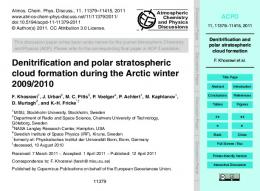
The PSCs that were simulated in the area of Kiruna were compared with the lidar measurements at Esrange and IRF Kiruna, respectively. A good agreement was found for all back trajectories. The PSCs were most pronounced both in the lidar measurements and box model simulations between the 22 and 24 January. Figure 6 shows one of the microAtmos. Chem. Phys., 11, 8471–8487, 2011

physical box model simulations where PSC formation was simulated at the start and end of the back trajectory. This simulation was performed at 23 January starting at Esrange at 19:00 UT at 22 km (the green trajectory in Fig. 5). The simulation starts at the end of the trajectory, thus at the location and time from where the air mass originated since the box model simulation is performed forward in time while the trajectories are calculated backward in time. Thus, the end of the simulation (from t = −30 h onwards) shows the PSC formation in the area of Kiruna. At t = −30 h TNAT is reached and the liquid H2 SO4 /H2 O particles start to take up HNO3 . As the temperature decreases further (almost reaching Tice ) more and more HNO3 is taken up and with a weight percentage of 40% HNO3 fully developed STS PSCs are formed. The simulation of a STS PSC at 22 km is in agreement with the lidar measurements with the Esrange lidar at this altitude as can be seen from Fig. 7. The figure shows the lidar measurement of backscatter in parallel and perpendicular polarisation on 23 January at 19:00 UT. A PSC that extended over the altitude range from 17.5 to 25.5 km was measured. The PSC consisted of two layers with maxima in parallel and perpendicular backscatter ratio at 20 and 24 km. The composition was mainly STS with some NAT and mixed layers at the bottom and top of the PSC. The simulations at 19 km and 25 km (not shown) are also in agreement with the lidar measurement at these altitudes. PSC occurrence in the Kiruna area was dominated by NAT in the beginning of January (3–7 January) and dominated by STS clouds (with some NAT and mixed layers in between as in Fig. 7) from mid January to end of January (11–20 January). Temperatures were generally for several hours below TNAT but never reached Tice . Uptake of HNO3 by the liquid H2 SO4 /H2 O aerosols and PSC type Ib (STS) formation occurred 10 h (17 January) and 40 h (24 January), respectively, before the lidar measurements were performed (Fig. 6). This indicates in agreement with the measurements that during that time period the same PSC persisted over Kiruna with differing strength. The PSC was most pronounced in the microphysical box model simulation between 22 and 24 January which also is in agreement with the lidar measurements performed in Kiruna. 4.3

PSC formation north of Scandinavia

For investigating PSCs that were simulated north of Scandinavia we have to focus on the time between t = −140 h and t = −110 h, thus at the begin of the box model simulation (Fig. 6). As the air mass passes over the sea between Scandinavia and Svalbard temperatures reach below Tice for approximately 15 h (Figs. 5 and 6). Due to these cold temperatures HNO3 is taken up and STS PSCs are formed. However, due to these low temperatures also formation of NAT and ice PSCs is possible which are not included in this simulation but will be discussed later based on measurements.


T_NAT T_ICE

B: B: B: B: B: B:

0 5 10 15 20 25

B: B: B: B: B: B:

0 5 10 15 20 25

B: B: B: B: B: B:

Fig. 7. Backscatter ratio in parallel (left) and with perpendicular (right) polarisation measured with the Esrange polarisation measured the Esrange lidar, 1-h integration time, lidar, 5

B: B: B: B: B: B:

0 5 10 15 20 25

Fig. 7. Backscatter ratio in parallel (left) and perpendicular (right) 0

10

starting at 19:02 on2323January January The colors markPSC thetypes. dif1-h time, starting at 19:02UT UT on 2010. 2010. The colors mark the different 15 integration 20 25

ferent PSC types. 2010-01-18

30 28 26 24 22 20 18 16

00:31:35 UTC M2 M2e Ice IceW

1.00

8481

PSC Composition

215 210 205 200 195 190 185 50 45 40 35 30 100 80 60 40 20 0 60 50 40 30 20 10 0 100 80 60 40 20 0 10.00

Altitude, km

r [μm]

H2SO4 [wt%]

HNO3 [wt%]

H2O [wt%]

p [hPa]

T [K]


STS M1

the trajectory approximately on 18 January. On that overpass CALIPSO observed a PSC that extended from 17 to 20 km up to 25 to 26 km (depending on latitude and longitude). The −60 −40 −20 0 69.95, 42.64 78.72, 66.23 60.00, 33.16 81.39, 129.72 4.44, 170.68 PSC was composed of(LaSTS, Mix-2 as well 7as ice partitude; LonMix-1, gitude) t [h] ticles which coincides with the temperatures below Tice as found along the back trajectories. Thus, though we do not Fig. 6. Microphysical box model simulation for the observation 22.8 .4 23 22.1 NAT and ice we know from the temperexplicitly at Esrange on 22 January 19:00 UT (22 km). Shown is the devel8 calculate 22. .1 22 ature history of the back trajectory and the CALIPSO meaopment of the temperature in K, the pressure in hPa, the weight fraction of water, nitric acid and sulfuric acid in wt % as well as the surements that in that area all three PSC types were present particle radius in µm for the different particle size classes denoted at the same22.8time. Further, this shows that the temperature by B0–B25 (B0 = smallest and B25 = largest size class). Note: the history derived from HYSPLIT based on NCEP analyses and simulations are performed forward in time, thus, the end of the simthe CALIPSO measurements are in agreement. The ice PSCs ulation coincides with the measurement and the starting point of during that time period were caused by a synoptic-scale coolFig. 8. CALIPSO PSC composition observation for the orbit starting on 18 January 2010 at 00:19 UT (top) and the trajectory. ing of the air mass as was discussed in Pitts et al. (2011). GEOS-5 temperatures and geopotential height fields at 30 hPa at 12:00 UT (right). The white line marks the 0.10 0.01 −140 −120 −100 −80

60N

182

190

198

206

214

222

230 238

GEOS5 Temperature, K

CALIPSO orbit track.

The occurrence of temperatures below Tice show that the air masses were originating from the regions where the center of the vortex with the coldest temperatures was located (north of Scandinavia). The temperatures along the back trajectories were for several hours below TNAT and reached also for some hours below Tice . PSC formation was simulated generally 130 to 90 h before the lidar measurements were performed. The PSC were most pronounced along the back trajectories started between 22 and 24 January (thus these show the PSC that occurred between 14 to 18 January north of Scandinavia). Since ground-based lidar measurements are not available at the locations where the back trajectories originate we compare these simulations with space-borne measurements from CALIPSO. Figure 8 shows the CALIPSO composition observation on 18 January at 00:19 UT. The CALIPSO track passes from east of Scandinavia northwards crossing the trajectory that was calculated on 23 January 6-days backward, thus crossing www.atmos-chem-phys.net/11/8471/2011/

4.4

PSC formation and denitrification 31

To investigate where exactly the cold temperatures generally occurred during the Arctic winter 2009/2010 and thus if these areas agree with the areas where ice PSCs and denitrification was observed, the coordinates where temperatures below Tice were encountered along the back trajectories are plotted on a map (Fig. 9). The trajectories that were started at Esrange as well as the trajectories that were started from IRF Kiruna are included. This figure shows that temperatures below Tice were reached above the sea west of Greenland on 2 January and at several locations northeast of Scandinavia (between Svalbard and Novaya Zemlya) on the 15, 17 and 18 January. Simulations with the Weather Forecasting and Research (WRF) model and the studies by Pitts et al. (2011) and Dörnbrack et al. (2011) showed mountain wave activity with subsequent ice PSC formation, respectively, around Atmos. Chem. Phys., 11, 8471–8487, 2011


00:31:35 UTC M2 M2e Ice IceW STS M1

Altitude, km

2010-01-18 30 28 26 24 22 20 18 16 69.95, 42.64

60.00, 33.16

78.72, 66.23 (Latitude; Longitude)

81.39, 129.72

PSC Composition

8482

74.44, 170.68

60N

22.8

.4 23 8 22. .1 22

22.1

22.8 182

190

198

206

214

230 238

222

GEOS5 Temperature, K

Fig. 8. CALIPSO PSC composition observation for the orbit starting on 18 January 2010 at 00:19 UT (top) and GEOS-5 temperatures and geopotential height fields at 30 hPa at 12:00 UT (right). The white line marks the CALIPSO orbit track. 150oW

18 o 0W

o 0W

12

70 o N

90 o W

o 0E 15

**¤¤ ¤

¤

o

30

**

W

¤

¤ ¤

¤ ¤¤ ¤ ¤ +++ ¤ ¤+ +++++ +++¤+ +¤+¤+**¤ +++***

¤¤ **¤**

*****+++*++*+++ **

0o

+++¤ *****

90 o E

o

60 W

120oE

80 o N

¤ o

60

E

o

30oE

Fig. 9. The locations where Tice along the back trajectories was encountered. The back trajectories that were started from IRF Kiruna are denoted with a star, the ones started from Esrange with a plus symbol and the CALIPSO measurements are denoted with circles. The dates when Tice was encountered are colour coded: 2 January (green), 15 January (magenta), 17 January (dark blue) and 18 January (light blue).

Atmos. Chem. Phys., 11, 8471–8487, 2011

Greenland in the beginning of January2 . Thus, while the temperatures below Tice were caused by mountain waves on 2 January they were caused by a synoptic-scale cooling for 15–18 January. The extension of low temperatures during this synoptic cooling can be seen from the temperatures that were simulated with WRF. Figure 10 shows the temperatures that were derived with WRF for the 17 and 18 January at 12:00 UT at the altitudes 18, 20 and 22 km. A large area (extending from Northern Scandinavia to Svalbard and Novaya Zemlya) reaching temperatures below Tice is found at 20 and 22 km. To compare the areas where Tice was encountered along the back trajectories with the locations where ice PSCs were observed by CALIPSO these locations were also included in Fig. 9. Note: only one coordinate pair (lat/lon) per ice PSC has been chosen (center of the cloud). The PSCs measured by CALIPSO agree well with the regions where Tice was found along the back trajectories. Further, the PSC formation north of Scandinavia agrees spatially and locally quite well with the area where gas-phase HNO3 removal was observed by Odin/SMR (compare Fig. 9 with Fig. 1). Thus, from this coincidence we suggest that ice formation on NAT particles could have occurred during that particular winter and that subsequent sedimentation of these particles could have caused the denitrification that was observed between 2 WRF simulations were carried out with versions 3.2 and 3.3 with ECMWF analyses as input data. The model simulations were performed on 92 vertical levels (up to 5 hPa) with varying height resolution (0.5 km or better in the stratosphere) and with a horizontal resolution of 3 km



8483

17 Jan

18 Jan

Temperatures at z=18km; 17/01/10 12:00 UT

Temperatures at z=18km; 18/01/10 12:00 UT 200

200

80° N

Ice

°

20 E

30° E

°

40 E

50° E

IC E

65° N ° 0

60° E

NA

T

10° E

°


40° E

30° E

20 E

185

S

ST

50° E

60° E 185


200

80° N

STS 190

E

30° E

40° E

50° E

10° E

20° E

185


Ice

ICE

S

ST

20° E

STS

65° N ° 0

60 E

E

E

°

10° E

190 IC

Ice

IC

ICE

ICE

S ST

65° N ° 0

ICE

ICE ICE

STS 70° N

ICE

IC

75° N

E IC

70° N

NAT

ICE

NAT 75° N

Temperature [K]

80° N

Temperature [K]

10 E

STS

S

ST

S ST

ST

S

S °

Ice

ICE

STS

NAT

IC E

S ST

STS

ST

65° N ° 0

70° N

ICE

70° N

STS E IC

E

ICE

IC

195

75° N

ICE

STS

Temperature [K]

E

ICE

IC

NAT E IC

75° N

195

ICE

ICE

NAT

Temperature [K]

80° N

°

40° E

30° E

50° E

60 E 185


200

80° N

80° N

IC E

ICE

E

10° E

°

20 E

30° E

°

40 E

50° E

60° E

65° N ° 0

Ice 185

ICE

IC IC E E

IC

65° N ° 0

STS

S

10° E

Temperature [K]

70° N

ST

20° E

ICE

STS

NAT

ICE

70° N

75° N

ICE

NAT

195

ICE

75° N

Temperature [K]

ICE 195

30° E

40° E

50° E

60° E

Ice 185

Fig. 10. Temperatures simulated with WRF on 17 (left column) and 18 January 2010 (right column) 12:00 UT at 18 (top), 20 (middle) and 22 km (bottom). white lines indicate the with areas WRF where ice, STS(left and column) NAT formation temperatures, respectively, are reached. Fig. 10. The Temperatures simulated on 17 and 18 January 2010 (right column) 12 UT at

18 (top), 20 (middle) and 22 km (bottom). The white lines indicate the areas where ice, STS and NAT formation 15–21temperatures, January. Pittsrespectively, et al. (2011)are found an increase in ice 26.4◦ E, 350 km East from Kiruna). The high-resolution reached. PSC observations with a coincident decrease in NAT mixin-situ measurements of the stratospheric gas-phase water ture observations indicating that heterogeneous nucleation on vapour were performed by two different hygrometers: The NAT particles may be an important mechanism for the formaFLASH-B optical fluorescent hygrometer (Yushkov et al., tion of synoptic-scale ice PSCs and thus their findings are in 1998) and the CFH frost point hygrometer (Vömel et al., 2000), showing close agreement between the data. The water agreement with our findings. vapour measurements were accompanied with aerosol in-situ During the second half of January 2010 a series of balloon observations by the COBALD backscatter sonde flown on the soundings were conducted from FMI (Finish Meteorologisame balloon. The obtained profiles revealed clear evidences ◦ cal Institute) Arctic Research Center in Sodankylä (67.3 N,

33 www.atmos-chem-phys.net/11/8471/2011/

Atmos. Chem. Phys., 11, 8471–8487, 2011

8484


of an irreversible dehydration with ice particles sedimenting and evaporating hundreds of meters below the initial level. The signatures of dehydration and rehydration in the water vapour vertical profiles were observed within the 18–24 km range between 17 and 29 January. Further, back trajectory analysis performed using HYSPLIT on ECMWF reanalysis suggests that the dehydration occurred primarily between 16 and 19 January and the dehydrated air masses were originating from the area North-East of Scandinavia where the coldest temperatures were observed. Back trajectory analysis performed using HYSPLIT trajectory model run on ECMWF reanalysis suggests that the dehydrated air masses were originating from the area north of Scandinavia where the coldest temperatures were observed (Khaykin et al., 2011). Thus, our finding and the findings by Pitts et al. (2011) are corroborated by these balloon measurements of H2 O made in Sodankylä showing dehydration. If denitrification was caused by sedimenting ice particles concurrent dehydration must occur. In contrast, for the denitrification that was observed between 9–15 January sedimenting NAT particles that formed on mountain wave ice PSCs as has been discussed by Fueglistaler et al. (2002), Dhaniyala et al. (2002) and Mann et al. (2005) could be a possible mechanism.

5

Conclusions

Denitrification was observed by Odin/SMR during the Arctic winter 2009/2010 between 475 to 525 K. A comparison of the Odin/SMR measurements for the last ten years shows that this was the strongest denitrification event in the entire Odin/SMR measuring period (2001–2010). Here, we use a combination of ground-based and space-borne lidar measurements together with microphysical box model simulations to investigate PSC formation and denitrification during the Arctic winter 2009/2010. Ground-based lidar measurements were performed in the area of Kiruna at IRF (67.8◦ N, 20.4◦ E) from 3 to 24 January and from 16 to 30 January at Esrange (67.8◦ N, 21.1◦ E), respectively. In the Kiruna area the PSCs were dominated by NAT in the beginning of January and by STS with some mixed or NAT layers at the bottom and/or top of the PSC. A distinct ice cloud was solely observed once, namely on 10 January by the IRF lidar in Kiruna. Trajectories were calculated with HYSPLIT based on the NCEP/GDAS meteorological analyses. The temperatures along the trajectories reached generally below TNAT for several hours but temperatures below Tice were only encountered occasionally when the air mass was transported over the areas north of Scandinavia, over the sea between Svalbard and Novaya Zemlya. In this region the center of the vortex was located that cooled down synoptically during the course of the winter to temperatures below Tice (15–21 January). MiAtmos. Chem. Phys., 11, 8471–8487, 2011

crophysical box model simulations along the HYSPLIT trajectories simulating STS cloud formation show that in case when the air mass passed the cold pool that PSC formation of PSCs type Ib (STS) can be simulated in the Kiruna area as well as North of Scandinavia. Due to the extremely low temperatures encountered north of Scandinavia, besides STS formation NAT and ice formation that has not been considered in the simulations can be expected in this area. In fact, NAT and ice PSCs were observed by CALIPSO in mid January north of Scandinavia. Comparison of the area where the trajectories encounter temperatures below Tice and measurements of ice PSCs by CALIPSO show that these areas are in good agreement. Further, this area is also collocated with the area where HNO3 removal by Odin/SMR was observed. Further, denitrification with accompanying renitrification was observed with Aura/MLS. Thus, this consistency suggests that during this particular winter denitrification between 15–21 January could have been caused by sedimenting ice particles that had formed on NAT particles. A denitrification caused by sedimenting ice particles occurs in general with a concurrent dehydration. Dehydration was observed by ballon measurements made from Sodankylä (67.3◦ N, 26.4◦ E). Trajectory analyses showed that the air masses were dehydrated between 16 and 19 January and that the dehydrated air was originating from the area north of Scandinavia where the cold temperatures were observed (Khaykin et al., 2011). Further, our results are in agreement with Pitts et al. (2011) who found an increase in ice PSC observations and coincident decrease in NAT mixture observations and suggested that this indicates heterogeneous nucleation of ice on NAT particles may be an important mechanism for the formation of synopticscale ice PSCs. In contrast, for the denitrification that was observed between 9–15 January sedimenting NAT particles that formed on mountain wave ice PSCs as has been discussed by Fueglistaler et al. (2002), Dhaniyala et al. (2002) and Mann et al. (2005) could be a possible mechanism. Acknowledgements. We are grateful to the European Space Agency (ESA) for providing the Odin/SMR data. Odin is a Swedish led project funded jointly by Sweden (SNSB), Canada (CSA), Finland (TEKES), and France (CNES) and the European Space Agency (ESA). The authors gratefully acknowledge the NOAA Air Resources Laboratory (ARL) for the provision of the HYSPLIT READY website (http://www.arl.noaa.gov/ready.php) used in this publication for calulating the trajectories. We would like to thank P. Konopka for the diffusive uptake code, P. Deuflhard and U. Nowak for providing the solver for ordinary differential equations used in the microphysical box model and M. Hervig for providing a program to calculate the NAT existence temperatures. Further, we would like to thank U. Blum for help with the PSC classification and analysis of the lidar data, R. Müller for helpful discussions and the two anonymous reviewer for helpful comments. Work at the Jet Propulsion Laboratory, California Institute of Technology, was done under contract with the National Aeronautics and Space Administration. WRF simulations were conducted using


F. Khosrawi et al.: Denitrification and polar stratospheric cloud formation the resources of the High Performance Computing Center North (HPC2N), Ume˚a, Sweden. We are also grateful to the Swedish Research Council for funding F. Khosrawi. Edited by: D. Knopf

References Achtert, P., Khosrawi, F., Blum, U., and Fricke, K.-H.: Investigation of polar stratospheric clouds in January 2008 by means of ground-based and space-borne lidar measurements and microphysical box model simualations, J. Geophys. Res., 116, D07201, doi:10.1029/2010JD014803, 2011. Biermann, U. M., Crowley, J. N., Huthwelker, T., Moortgat, G. K., Crutzen, P. J., and Peter, T.: FTIR studies on lifetime prolongation of stratospheric ice particles due to NAT coating, Geophys. Res. Lett., 21, 3939–3942, doi:10.1029/1998GL900040, 1998. Blum, U. and Fricke, K. H.: The Bonn University lidar at the Esrange: technical description and capabilities for atmospheric research, Ann. Geophys., 23, 1645–1658, 2005, http://www.ann-geophys.net/23/1645/2005/. Blum, U., Fricke, K. H., Müller, K. P., Siebert, J., and Baumgarten, G.: Long-term lidar observations of polar stratospheric clouds at Esrange in Northern Sweden, Tellus B, 57, 412–422, 2005. Blum, U., Khosrawi, F., Baumgarten, G., Stebel, K., Müller, R., and Fricke, K. H.: Simultaneous lidar observations of a polar stratospheric cloud on the east and west sides of the Scandinavian mountains and microphysical box model simulations, Ann. Geophys., 24, 3267–3277, doi:10.5194/angeo-24-3267-2006, 2006. Browell, E. V., Butler, C. F., Ismail, S., Robinette, P. A., Carter, A. F., Higdon, N. S., Toon, O. B., Schoeberl, M., and Tuck, A. F.: Airborne LIDAR observations in the wintertime Arctic stratosphere: polar stratospheric clouds, Geophys. Res. Lett., 17, 385–388, 1990. Carslaw, K. S., Luo, B. P., Clegg, S. L., Peter, T., Brimblecombe, P., and Crutzen, P. J.: Stratospheric aerosol growth and HNO3 gas phase depletion from coupled HNO3 and water uptake by liquid particles, Geophys. Res. Lett., 21, 2479–2482, 1994. Crutzen, P. J. and Arnold, F.: Nitric acid cloud formation in the cold Antarctic stratosphere: a major cause for the springtime “ozone hole”, Nature, 342, 651–655, 1986. Dhanilaya, S., McKinney, A., and Wennberg, O.: Lee-wave clouds and denitrification of the polar stratosphere, Geophys. Res. Lett., 29, 1322, doi:10.1029/2001GL013900, 2002. Dibb, J. E., Scheuer, E., Avery, M., Plant, J., and Sachse, G.: In situ evidence for renitrification in the Arctic lower stratosphere during the polar aura validation experiment (PAVE), Geophys. Res. Lett., 33, L12815, doi:10.1029/2006GL026243, 2006. Dörnbrack, A., Pitts, M. C., and Poole, L. R.: The winter Arctic stratosphere in 2009/2010 – overview, gravity wave activity and predictability of sudden stratospheric warmings, Atmos. Chem. Phys. Discuss., 11, in preparation, 2011. Drdla, K. and Browell, E. V.: Microphysical modeling of the 1999–2000 Arctic winter: 3. impact of homogeneous freezing on polar stratospheric clouds, J. Geophys. Res., 109, D10201, doi:10.1029/2003JD004352, 2004. Drdla, K. and Turco, R. P.: A 1-D model incorporating temperature oscillations, J. Atmos. Chem., 12, 319–366, 1991.


8485

Fahey, D. W., Kelly, K. K., Kawa, S. R., Tuck, A. F., Loewenstein, M., Chan, K. R., and Heid, L. E.: Observations of denitrification and dehydration in the winter polar stratosphere, Nature, 344, 321–324, 1990. Fahey, D. W., Gao, R. S., Carslaw, K. S., Kettleborough, J., Popp, P. J., Northway, M. J., Holecek, J. C., Ciciora, S. C., McLaughlin, R. J., Thompson, T. L., Winkler, R. H., Baumgardner, D. G., Gandrud, B., Wennberg, P. O., Dhaniyala, S., McKinley, K., Peter, T., Salawitch, R. J., Bui, T. P., Elkins, J. W., Webster, C. R., Atlas, E. L., Jost, H., Wilson, J. C., Herman, R. L., Kleinböhl, A., and von König, M.: The detection of large HNO3 containing particles in the winter Arctic stratosphere, Science, 291, 1026–1031, 2001. Fueglistaler, S., Luo, B. P., Voigt, C., Carslaw, K. S., and Peter, Th.: NAT-rock formation by mother clouds: a microphysical model study, Atmos. Chem. Phys., 2, 93–98, doi:10.5194/acp2-93-2002, 2002. Hanson, D. R. and Mauersberger, K.: Laboratory studies of the nitric acid trihydrate: implications for the south polar stratosphere, Geophys. Res. Lett., 15, 855–858, 1988. Irie, H., Koike, M., Kondo, Y., Bodeker, G. E., G., Danilin, M. Y., and Sasano, Y.: Redistribution of nitric acid in the Arctic lower stratosphere during the winter of 1996–1997, J. Geophys. Res., 106(D19), 23139–23150, 2001. Jimńez, C., Pumphrey, H. C., MacKenzie, I. A., Manney, G. L., Santee, M. L., Schwartz, J., Harwood, R. S. and Waters, J. W.: EOS MLS observations of dehydration in the 2004–2005 polar winters, Geophys. Res. Lett., 33, L16806, doi:10.1029/2006GL025926, 2006. Khaykin, S. Engel, I., Hoyle, C., Luo, B. P., Wienhold, F., Peter, Th., Kivi, R., Lykov, A., Yushkov, V., Shur, G., Poole, L., Spelten, N., Schiller, C., Voemel, H., Naebert and et al.: Dehydration and ice PSCs in the Arctic stratosphere: a case study based on accurate in-situ measurements, in preparation, 2011. Khosrawi, F. and Konopka, P.: Enhancement of nucleation and condensation rates due to mixing processes in the tropopause region, Atmos. Environ., 37, 903–910, 2003. Khosrawi, F., Ström, J., Minikin, A., and Krejci, R.: Particle formation in the Arctic free troposphere during the ASTAR 2004 campaign: a case study on the influence of vertical motion on the binary homogeneous nucleation of H2 SO4 /H2 O, Atmos. Chem. Phys., 10, 1105–1120, doi:10.5194/acp-10-1105-2010, 2010. Knopf, D. A., Koop, T., Luo, B. P., Weers, U. G., and Peter, T.: Homogeneous nucleation of NAD and NAT in liquid stratospheric aerosols: insufficient to explain denitrification, Atmos. Chem. Phys., 2, 207–214, doi:10.5194/acp-2-207-2002, 2002. Kondo, Y., Irie, H., Koike, M., and Bodeker, G. E.: Denitrification and nitrification in the Arctic stratosphere during the winter of 1996–1997, Geophys. Res. Lett., 27(3), 337–340, 2000. Koop, T., Biermann, U. M., Raber, W., Luo, B. P., Crutzen, P. J., and Peter, T.: Do stratospheric aerosol droplets freeze above the ice frost point?, Geophys. Res. Lett., 22, 917–920, 1995. Koop, T., Carslaw, K. S., and Peter, T.: Thermodynamic stability and phase transitions of PSC particles, Geophys. Res. Lett., 24, 2199–2202, 1997. Koop, T., Luo, B., Tsias, A., and Peter, T.: Water activity as the determinant for homogeneous ice nucleation in aqueous solutions, Nature, 406, 611–614, 2000. Larsen, N., Knudsen, B. M., Rosen, J. M., Kjome, N. T., Neuber, R.,

Atmos. Chem. Phys., 11, 8471–8487, 2011

8486


and Kyrö, E.: Temperature histories in liquid and solid polar stratospheric cloud formation, J. Geophys. Res., 102, 23505– 23517, 1997. Larsen, N., Hoyer Svendsen, S., Knudsen, B. M., Mikkelsen, I. S., Voigt, C., Kohlmann, A., Schreiner, J., Mauersberger, K., Deshler, T., Kröger, C., Rosen, J. M., Kjome, N. T., Adriani, A., Cairo, F., Di Donfrancesco, G., Ovarlez, J., Ovarlez, H., Dörnbrack, A., and Birner, T.: Microphysical mesoscale simulation of polar stratospheric cloud formation constrained by in situ measurements of chemical and optical cloud properties, J. Geophys. Res., 107, 8301, doi:10.1029/2001JD000999, 2002. Larsen, N., Knudsen, B. M., Svendsen, S. H., Deshler, T., Rosen, J. M., Kivi, R., Weisser, C., Schreiner, J., Mauerberger, K., Cairo, F., Ovarlez, J., Oelhaf, H., and Spang, R.: Formation of solid particles in synoptic-scale Arctic PSCs in early winter 2002/2003, Atmos. Chem. Phys., 4, 2001–2013, doi:10.5194/acp-4-2001-2004, 2004. Livesey, N. J., Read, W. G., Froidevaux ,L., Lambert, A., Manney, G. L., Pumphrey, H. C., Santee, M. L., Schwartz, M. J., Wang, S., Cofield, R. E., Cuddy, D. T., Fuller, R. A., Jarnot, R. F., Jiang, J. H., Knosp, B. W., Stek, P. C., Wagner, P. A., and Wu, D. L.: Aura Microwave Limb Sounder (MLS) Version 3.3 Level 2 data quality and description document, JPL D-33509, available at: http://mls.jpl.nasa.gov/, 2011. Lowe, D. and MacKenzie, R.: Review: Polar stratospheric cloud microphysics and chemistry, J. Atmos. Sol.-Terr. Phys., 70, 13– 40, 2008. Luo, B., Carslaw, K. S., Peter, T., and Clegg, S. L.: Vapour pressures of H2 SO4 /HNO3 /HCl/HBr/H2 O solutions to low stratospheric temperatures, Geophys. Res. Lett., 22, 247–250, 1995. Mann, G. W., Carslaw, K. S., Chipperfield, M. P., Davies, S., and Eckermann, S. D.: Large nitric acid trihydrate particles and denitrification cuased by mountain waves in the Arctic stratosphere, J. Geophys. Res., 110, D08202, doi:10.1029/2004JD005271, 2005. Marti, J. and Mauersberger, K.: A survey and new measurements of ice vapor pressure temperatures between 170 and 250 K, Geophys. Res. Lett., 20, 363–366, 1993. McCormick, M. P., Steele, H. M., Hamill, P., Chu, W. P., and Swissler, T.: Polar stratospheric cloud sightings by SAM II, J. Atmos. Sci., 39, 1387–1397, 1982. Meilinger, S., Koop, K., Luo, B. P., Huthwelker, T., Carslaw, K. S., Krieger, U., Crutzen, P. J., and Peter, T.: Size-dependent stratospheric droplet composition in lee wave temperature fluctuations and their potential role in PSC freezing, Geophys. Res. Lett., 22, 3031–3034, 1995. Murtagh, D., Frisk, U., Merino, F., Ridal, M., Jonsson, A., Stegman, J., Witt, G., Eriksson, P., Jimenez, C., Megie, G., de la Noe, J., Ricaud, P., Baron, P., Pardo, J. R., Hauchcorne, A., Llewellyn, E. J., Degenstein, D. A., Gattinger, R. L., Lloyd, N. D., Evans, W. F. J., McDade, I. C., Haley, C. S., Sioris, C., von Savigny, C., Solheim, B. H., McConnell, J. C., Strong, K., Richardson, E. H., Leppelmeier, G. W., Kyrola, E., Auvinen, H., and Oikarinen, L.: An overview of the Odin atmospheric mission, Can. J. Phys., 80, 309–319, 2002. Ovarlez, J. O. and Ovarlez, H.: Stratospheric water vapor content evolution during EASOE, Geophys. Res. Lett., 21, 1235–1238, 1994. Pagan, K. L., Tabazadeh, A., Drdla, K., Hervig, M., Ecker-

Atmos. Chem. Phys., 11, 8471–8487, 2011

mann, S. D., Browell, E. V., Legg, M. L., and Froschi, P. G.: Observational evidence against mountain wave-wave generation of ice nuclei as prerequisite for the formation of three solid nitric acid polar stratospheric clouds observed in the Arctic in early December 1999, J. Geophys. Res., 109, D04312, doi:10.1029/2003JD003846, 2004. Pawson, S., Naujokat, B., and Labitzke, K.: On the polar stratospheric cloud formation potential on the northern stratosphere, J. Geophys. Res., 104, 14209–14222, 1995. Peter, T.: Microphysics and heterogeneous chemistry of polar stratospheric clouds, Annu. Rev. Phys. Chem., 48, 785–822, 1997. Pitts, M. C., Thomason, L. W., Poole, L. R., and Winker, D. M.: Characterization of Polar Stratospheric Clouds with spaceborne lidar: CALIPSO and the 2006 Antarctic season, Atmos. Chem. Phys., 7, 5207–5228, doi:10.5194/acp-7-5207-2007, 2007. Pitts, M. C., Poole, L. R., and Thomason, L. W.: CALIPSO polar stratospheric cloud observations: second-generation detection algorithm and composition discrimination, Atmos. Chem. Phys., 9, 7577–7589, doi:10.5194/acp-9-7577-2009, 2009. Pitts, M. C., Poole, L. R., Drnbrack, A., and Thomason, L. W.: The 2009–2010 Arctic polar stratospheric cloud season: a CALIPSO perspective, Atmos. Chem. Phys., 11, 2161–2177, doi:10.5194/acp-11-2161-2011, 2011. Poole, L. R. and McCormick, M. P.: Polar stratospheric clouds and the Antarctic ozone hole, J. Geophys. Res., 93, 8423–8430, 1988. Pruppacher, H. and Klett, J. D.: Microphysics of Clouds and Precipitation, D. Reidel, Norwell, MS, 1978. Salcedo, D., Molina, L. T., and Molina, M. J.: Homogeneous freezing of concentrated aqueous nitric acid solutions at polar stratospheric temperatures, J. Phys. Chem., 105, 1433–1439, 2001. Santee, M., Manney, G., Livesey, N., and Read, W.: Threedimensional structure and evolution of HNO3 based on UARS Microwave Limb Sounder measurements, J. Geophys. Res., 109, D15206, doi:10.1029/2004JD004578, 2004. Santee, M., Lambert, A., Read, W. G., Livesey, N. J., Cofield, R. E., Cuddy, D. T., Daffer, W. H., Drouin, B. J., Froidevaux, L., Fuller, R. A., Jarnot, R. F., Knosp, B. W., Manney, G. L., Perun, V. S., Snyder, W. V., Stek, P. C., Thurstans, R. P., Wagner, P. A., Waters, J. W., Muscari, G., de Zafra, R. L., Dibb, J. E., Fahey, D. W., Popp, P. J., Marcy, T. P., Jucks K. W., Toon, G. C., Stachnik, R. A., Bernath, P. F., Boone, C. D., Walker, K. A., Urban, J. and Murtagh, D.: Validation of the Aura Microwave Limb Sounder HNO3 measurements, J. Geophys. Res., 112, D24S40, doi:10.1029/2007JD008721, 2007. Solomon, S.: Stratospheric ozone depletion: a review of concepts and history, Rev. Geophys., 37, 275–316, 1999. Solomon, S., Garcia, R. R., Rowland, F. S., and Wuebbles, D. J.: On the depletion of Antarctic ozone, Nature, 321, 755–758, 1986. Steele, H. M., Hamill, P., McCormick, M. P., and Swissler, T. J.: The formation of polar stratospheric clouds, J. Atmos. Sci., 40, 2055–2067, 1983. Tabazadeh, A., Toon, O. B., and Hamill, P.: Freezing behaviour of stratospheric sulfate aerosols inferred from trajectory studies, Geophys. Res. Lett., 22, 1725–1728, 1995. Tabazadeh, A., Toon, O. B., Gary, B. L., Bacmeister, J. T., and Schoeberl, M. R.: Observational constraints on the formation of type 1a polar stratospheric clouds, Geophys. Res. Lett., 23, 2109–2112, 1996.


F. Khosrawi et al.: Denitrification and polar stratospheric cloud formation Toon, O. B., Hamil, P., Turco, R. P., and Pinto, J.: Condensation of HNO3 and HCl in winter polar stratospheres, Geophys. Res. Lett., 13, 1284–1287, 1986. Toon, O. B., Tabazadeh, A., and Browell, E. V.: Analyses of lidar observations of Arctic polar stratospheric clouds during January 1989, J. Geophys. Res., 105, 20589–20615, 2000. Urban, J., Lautié, N., Le Flochmoën, E., Jiménez, C., Eriksson, P., De La Noë, J., Dupuy, E., Ekström, M., El Amraoui, L., Frisk, U., Murtagh, D., Olberg, M., and Ricaud, P.: Odin/SMR limb observations of stratospheric trace gases: level 2 processing of ClO, N2 O, HNO3 , and O3 , J. Geophys. Res., 110, D14307, doi:10.1029/2004JD005741, 2005. Urban, J., Murtagh, D., Lautié, N., Barret, B., Dupuy, E., De La Noë, J., Eriksson, P., Frisk, U., Jones, A., Le Flochmoën, E., Olberg, M., Piccolo, C., Ricaud, P., and Rösevall, J.: Odin/SMR limb observations of trace gases in the polar lower stratosphere during 2004–2005, in: Proceedings of the ESA First Atmospheric Science Conference, 8–12 May 2006, Frascati, Italy, edited by: H. Lacoste, Eur. Space Agency Spec. Publ., 2006. Urban, J., Pommier, M., Murtagh, D. P., Santee, M. L., and Orsolini, Y. J.: Nitric acid in the stratosphere based on Odin observations from 2001 to 2009 – Part 1: A global climatology, Atmos. Chem. Phys., 9, 7031–7044, doi:10.5194/acp-9-7031-2009, 2009. Voigt, C., Schreiner, J., Kohlmann, A., Zink, P., Mauersberger, K., Larsen, N., Deshler, T., Kröger, C., Rosen, J., Adriani, A., Cairo, F., Donfrancesco, G. D., Viterbini, M., Ovarlez, J., Ovarlez, H., David, C., and Dörnbrack, A.: Nitric acid trihydrate (NAT) in polar stratospheric clouds, Science, 290, 1756–1758, 2000. Voigt, C., Schlager, H., Luo, B. P., Dörnbrack, A., Roiger, A., Stock, P., Curtius, J., Vössing, H., Borrmann, S., Davies, S., Konopka, P., Schiller, C., Shur, G., and Peter, T.: Nitric Acid Trihydrate (NAT) formation at low NAT supersaturation in Polar Stratospheric Clouds (PSCs), Atmos. Chem. Phys., 5, 1371– 1380, doi:10.5194/acp-5-1371-2005, 2005. Vömel, H., Rummukainen, M., Kivi, R., Karhu, J., Turunen, T., Kyrö, E., Rosen, J., Kjome, N., and Oltmans, S.: Dehydration and sedimentation of ice particles in the Arctic stratospheric vortex, Geophys. Res. Lett., 24, 798–798, 1997.


8487

Vömel, H., David, D. E., and Smith, K.: Accuracy of tropospheric and stratospheric water vapor measurements by the cryogenic frost point hygrometer Instrumental details and observations, J. Geophys. Res., 112, D08305, doi:10.1029/2006JD007224, 2000. von Hobe, M., Grooss, J. U., Pope, F., Peter, T., Cairo, F., Orsolini, Y., Volk, C. M., Marchand, D. M., Janosi, I. M., Schlager, H., Stroh, F., Rex, M., Wienhold, F., et al.: Reconcilation of essential process parameters for an enhanced predictibility of Arctic stratospheric ozone loss and its climate interactions, Atmos. Chem. Phys. Discuss., 11, in preparation, 2011. Waters, J. W., Froidevaux, L., Harwood, R. S., Jarnot, R. F., Pickett, H. M., Read, W. G., Siegel, P. H., Cofield, R. E., Filipiak, M. J., Flower, D. A., Holden, J. R., Lau, G. K. K., Livesey, N. J., Manney, G. L., Pumphrey, H. C., Santee, M. L., Wu, D. L., Cuddy, D. T., Lay, R. R., Loo, M. S., Perun, V. S., Schwartz, M. J., Stek, P. C., Thurstans, R. P., Boyles, M. A., Chandra, K. M., Chavez, M. C., Chen, G. S., Chudasama, B. V., Dodge, R., Fuller, R. A., Girard, M. A., Jiang, J. H., Jiang, Y. B., Knosp, B. W., LaBelle, R. C., Lam, J. C., Lee, K. A., Miller, D., Oswald, J. E., Patel, N. C., Pukala, D. M., Quintero, O., Scaff, D. M., Van Snyder, W,. Tope, M. C., Wagner, P. A., and Walch, M. J.: The Earth Observing System Microwave Limb Sounder (EOS MLS) on the Aura satellite, IEEE T. Geosci. Remote Sens., 44, 1075–1092, 2006. Winker, D. M., Hunt, W. H., and McGill, M.: Initial performance assessment of CALIOP, Geophys. Res. Lett., 34, L19803, doi:10.1029/2007GL030135, 2007. Yushkov, V., Merkulov, S. and Astakhov V.: Optical balloon hygrometer for upper stratosphere and stratosphere water vapour measurements, in Optical remote sensing of the atmosphere and clouds edited by J.Wang, B.Wu, T.Ogawa, Z-h.Guans, Proc. SPIE, 3501, 439–445, 1998. Zondlo, M. A., Hudson, P. K., Prenni, A. J., and Tolbert, M. A.: Chemistry and microphysics of polar stratospheric clouds and cirrus clouds, Annu. Rev. Phys. Chem., 51, 473–499, 2000.

Atmos. Chem. Phys., 11, 8471–8487, 2011