Dense Graphs, Node Sets, and Riders: Toward a Foundation for Particle Physics without Continuum Mathematics Alexander G. D. Lamb
1545 Scenic Avenue Berkeley, CA 94708, USA
[email protected] Digital physics seeks to help answer problematic open questions in quantum gravity by bringing to bear techniques from computer science. One approach to this endeavor is the creation of a toolbox of algorithms that can reliably simulate basic quantum phenomena. To facilitate this goal, we explore the extent to which set-based, pseudo-particle algorithms and dense, irregular graphs can be made to emulate the behaviors of naturally occurring fundamental particles. We investigate the relation between dense graphs and pseudo-particles traversing them, which has profound implications for limits on particle information and may provide an experimental tool for testing the geometric properties of quantized space. We also show that behaviors with properties such as particle polarization are easy to generate with this approach.
1. Introduction
Many theorists in modern particle physics are investigating discrete models of spacetime in an attempt to reconcile quantum mechanics with general relativity~two theories that have resisted integration for almost a century [1, 2]. Computationally speaking, discrete models of nature are highly appealing for their simplicity, rigor, and firm logical foundation. Digital physics represents an attempt by the computer science community to meet these efforts halfway by providing new algorithmic tools for exploring such models. From a computational perspective, the universe may be said to be equivalent to some machine, be it a Turing machine, or some variety of hypercomputer. In this context, the aim of digital physics is to determine the computational requirements of such a universe machine and propose implementations, which are models that equate to sets of physical laws. Such implementations differ from normal formulaic descriptions of nature in that they always propose concrete mechanisms for natural processes with the understanding that such mechanisms may be ruled out if they do not match observation. One approach to the digital physics challenge is provided by the work of the New Kind of Science (NKS) movement. The NKS methodology is to explore the space of simplest possible algorithms in an unbiased fashion, so as to seek out those algorithms that are applicable Complex Systems, 19 © 2010 Complex Systems Publications, Inc. to a range of problems in science [3]~in this arena, specifically to particle physics. In contrast, the approach adopted by most particle physicists is to describe observed natural phenomena using the most expres-
A. G. D.byLamb approach to the digital physics challenge is provided the work of the New Kind of Science (NKS) movement. The NKS methodology is to explore the space of simplest possible algorithms in an unbiased fashion, so as to seek out those algorithms that are applicable to a range of problems in science [3]~in this arena, specifically to particle physics. In contrast, the approach adopted by most particle physicists is to describe observed natural phenomena using the most expressive and accurate mathematical toolkit available, regardless of the computational implications. To date, the most heavily used such toolkit has been continuum mathematics. Physicists then can encode these descriptions as computer simulations tuned to provide results at some given level of precision. A challenge for the NKS approach is that the search-space of possible universe implementations is vast. Thus, an unbiased exploration of this space may not be the most efficient means of identifying the best candidates for an algorithm that can compute nature. Furthermore, without an interpretive framework inspired by observations, it may be difficult to demonstrate that a given algorithm has relevance to physical systems. On the other hand, the toolkit of choice for most modern physics, namely continuum mathematics, may not be the right toolkit for constructing a successful implementation of the universe. The algorithmic approximations to nature that are produced by the implementation of physical formulas are a reflection of human toolbuilding and may be a poor model for an implementation of nature itself. For example, physical formulas do not generally provide an explicit model for how information is transferred through the universe. Also, these formulas are typically not constrained to be local, even while locality often plays a critical role in the theories themselves. Branches of physics such as quantum field theory assume the spontaneous transfer of information through fields over arbitrary distances while relying on an implicit and undefined mechanism for its propagation. Such approaches do not give weight to the fact that a field that extends indefinitely through smooth space contains an infinite amount of information and is therefore not computable. Broadly speaking, the principle that an object is only influenced by its immediate surroundings has played a critical role in the development of physical theory. This principle is only broken by quantummechanical systems, in which it is trumped by entanglement~ another, even more concrete form of informational connectedness. Ideally then, a computational model of physical phenomena would respect locality, while perhaps also describing both locality and entanglement through the same mechanism. Two strengths of the NKS approach are that it always provides an explicit mechanism for information transfer and that this mechanism is always local. This paper uses an intermediate approach between the NKS methodology and that of most physics. It seeks to preserve the concrete and local aspects of the NKS approach, without confining itself to the absolute simplest algorithms. At the same time, it attempts to produce particles that unambiguously resemble their natural analogs. The goal is to provide a discrete, local, deterministic, and Turingmachine-equivalent implementation for Publications, realistic particles. We do not Complex Systems, 19 © 2010 Complex Systems Inc. expect this particular implementation to be the actual one run by the universe. However, by exploring the space of plausible implementations, we hope to learn more about the actual implementation of the 116One
Dense Graphs, Node Sets, and Riders
117
The goal is to provide a discrete, local, deterministic, and Turingmachine-equivalent implementation for realistic particles. We do not expect this particular implementation to be the actual one run by the universe. However, by exploring the space of plausible implementations, we hope to learn more about the actual implementation of the universe than can be learned by simply generating a formulaic description. If this approach succeeds in producing relevant models of physical phenomena, it may then be possible to refine the resulting algorithms with an eye toward the NKS goal of finding the simplest such algorithms. We began an exploration of this approach in [4]. That paper tackled the following challenge: is it possible to create stable, local patterns that travel across a discrete approximation to space in a rotationally invariant fashion? We presented the “Jellyfish” algorithm and used it to produce a stable pseudo-particle that shows the desired behavior when applied to dense, irregular graphs. We also illustrated how motion around potential wells and a simple model of relativistic time dilation might be achieved using the same mechanisms. Arguably, the most interesting possibility to emerge from [4] was an indication that, for a given pseudo-particle size, there is a certain density of graph connections for which its motion is straightest. This leads to the possibility that models of this sort might eventually provide an experimentally testable measure of the granularity of space. For example, the scale and motion of electrons are well understood. It might be possible to make an estimate of the required connectedness of the spatial graph that electrons would have to traverse in order for their observed motion to be achieved, presuming that an algorithm in the same class as Jellyfish underpinned their motion. Such an investigation would be unlikely to prove useful, however, if the dense graphs approach is unable to yield particle behaviors rich enough to mirror those of actual electrons. This paper represents the first of several ongoing explorations into ways in which the dense graphs paradigm can be extended to bring it closer to observed phenomena. Of the numerous ways in which the current models fall short of mimicking nature, perhaps the easiest to amend is that of “particle complexity”. By this we refer to the physical attributes that fundamental particles exhibit, such as spin, charge, and polarization. The pseudo-particles generated in [4] were the simplest possible implementations: they had no intrinsic properties (other than size) and contained no substructure. It is useful, therefore, to extend our models to see how much information must be added to a pseudo-particle before it becomes plausibly naturalistic. In this paper, we explore in greater detail the relation between particle size and degree of graph connectedness suggested in [4]. This results in a concrete demonstration that for a given pseudo-particle size, there is an optimum degree of graph connectedness. We then attempt to extend our pseudo-particle model so that we may begin to put a minimum bound on the amount of information a natural particle requires to function. To Systems, achieve19this extension the model, we augComplex © 2010 ComplexofSystems Publications, Inc. ment the Jellyfish pseudo-particle algorithm previously described through the use of a mechanism we refer to as a “steed|rider” relationship. This mechanism is intended to represent a very simple relation-
In this paper, we explore in greater detail the relation between particle size and degree of graph connectedness suggested in [4]. This results in a concrete demonstration that for a given pseudo-particle size, 118 G. D. Lamb there is an optimum degree of graph connectedness. We A. then attempt to extend our pseudo-particle model so that we may begin to put a minimum bound on the amount of information a natural particle requires to function. To achieve this extension of the model, we augment the Jellyfish pseudo-particle algorithm previously described through the use of a mechanism we refer to as a “steed|rider” relationship. This mechanism is intended to represent a very simple relationship between two pseudo-particles. In this relationship, particle A (the rider) has information about the elements of particle B, while B (the steed) has no knowledge of A. Nodes referenced by A are a subset of those referenced by B. For the purposes of this work, the steed is an ordinary pseudo-particle of the sort explored in [4]. The rider is defined by a new, modified algorithm. The latter half of this paper explores in detail our first extension to the Jellyfish algorithm, which is designed to have behavior in common with the property of polarization seen in natural particles. The goal is to implement this behavior without impacting the straightness of motion that was achieved in [4]. Section 2 presents the relation between optimum particle size and the connectedness of the graph. The data suggests a linear increase in graph connectedness as a function of particle size. Section 3 proposes a definition for polarization in the context of pseudo-particle simulations and describes the rider algorithm used to create the effect, along with the metric used to test its effectiveness. A set of simulations designed to test the rider’s performance are described along with the results of the tests. Section 4 contains a discussion of the implications of this research. Section 5 briefly outlines some further simulations that are currently in progress, and Section 6 summarizes our conclusions.
2. Establishing Preconditions for Pseudo-Particle Behavior 2.1 Angular Deviation as a Measure of Straightness of Motion
As suggested in [4], given a pseudo-particle size n, there is an optimum graph connection density that produces the straightest linear motion (i.e., the least angular deviation from a straight path). We can characterize graph connection density as the average number of neighbors to a given node in the graph, or the “mean degree” for a node Xd\. We denote the optimum such density as Xd\opt . The relation between n and graph connection density Xd\opt was investigated in [4] using two-dimensional (2D) graphs, with relatively coarse sampling of the parameter space. However, the implementations of polarization-like behavior in Section 3 of this paper only become meaningful in three-dimensional (3D) graphs. We therefore begin this work by following up the preliminary 2D study of [4] with a higher density sampling of parameter space, and further extending this to 3D graphs. Performing a 3D parameter exploration requires generating graphs with a greatly increased total node count because we need to pack volumes with nodes instead of areas. However, holding enough nodes in computer memory to carry outSystems robustPublications, 3D simulations rapidly beComplex Systems, 19 © 2010 Complex Inc. comes awkward. To resolve this problem, new software was produced that made use of an “as-needed” graph construction technique. Under the new system, rather than creating an entire graph at runtime
Dense Graphs, Node and Riders 119 Performing a 3DSets, parameter exploration requires generating graphs with a greatly increased total node count because we need to pack volumes with nodes instead of areas. However, holding enough nodes in computer memory to carry out robust 3D simulations rapidly becomes awkward. To resolve this problem, new software was produced that made use of an “as-needed” graph construction technique. Under the new system, rather than creating an entire graph at runtime and wrapping the edges to produce a closed surface, we instead generate small tiles of the graph only as required when a pseudo-particle traverses them. To mimic the effect of randomly distributed nodes with a mean density of Xr\ nodes per tile, graph tiles were populated with varying numbers of nodes according to a Poisson distribution centered at Xr\. The nodes within each tile were then linked using a threshold neighbor radius r, as in [4]. This produced the effect of an unbounded topologically flat space. 2.2 Simulations for Determining Optimal Graph Density
Using the Jellyfish algorithm, we generated a set of simulations for a range of particle sizes with n 20 through 200, each with a range of degrees of graph node density Xr\ 20 through 571. For each value of n, we plotted the angular deviation qdev for each Xr\ value. qdev is defined as the net change in direction of pseudo-particle flight between the first half of a simulation sample run, and the second half (see [4] for details). Thus, lower values of qdev correspond to straighter motion. For each value of n, we determined the optimal value of Xr\ by fitting polynomial functions to the function qdev HXr\L and locating the value of Xr\ that corresponds to the minimum value of qdev . We call this value Xr\opt . As an example, Figure 1(a) shows the 2D simulations for n 80. There is a clear minimum in qdev at Xr\ 160 indicating that this graph density gives the straightest motion for a particle of size n 80. This minimum is due to two competing effects. At low Xr\, there are an insufficient number of nodes in the pseudo-particle front set candidates to adequately define forward motion. As Xr\ increases, the graph is more likely to have nodes where the pseudo-particle requires them to produce forward motion. The second effect applies at high Xr\, where each pseudo-particle element is connected to so many candidate nodes that are greater than n candidates with the same score. The pseudo-particle has no extra information for determining forward motion and so a random component is introduced. In Figure 1(b) we see the same behavior at n 160, with the minimum moving to a higher Xr\opt . Generally, we see that Xr\opt increases with n. However, as Xr\opt increases it becomes harder to ascertain the correct value because the simulations have only been run to Xr\ 571. For high n, we can only derive a lower bound for Xr\opt . It is also worth noting that for higher n, the relation between qdev and Xr\ around the minimum becomes broad and shallow. This Complex Systems, © viable 2010 Complex Publications, Inc. means that at high n, the range19of graph Systems densities for straightline motion becomes larger.
mum moving to a higher Xr\opt . Generally, we see that Xr\opt increases with n. However, as Xr\opt increases it becomes harder to as120 A. G.been D. Lamb certain the correct value because the simulations have only run to Xr\ 571. For high n, we can only derive a lower bound for Xr\opt . It is also worth noting that for higher n, the relation between qdev and Xr\ around the minimum becomes broad and shallow. This means that at high n, the range of viable graph densities for straightline motion becomes larger. Figure 2 shows Xr\opt for n 80 in the 3D case. Compared to the 2D case in Figure 1(a), Xr\opt is higher in three than in two dimensions. This was expected as the nodes in the graph need to populate a volume rather than an area. This means that we run up against the simulation limit faster in three dimensions and therefore will have more lower-bound points on Xr\opt in three than in two dimensions.
HaL
HbL
Figure 1. Example plots showing identification of Xr\opt for (a) n 80 and
(b) n 160 from a range of Xr\ values for two dimensions. Plot minima such as this were used to determine the relationship between n and Xr\opt .
Figure 2. Example plot showing identification of Xr\opt for n 80 from a
range of Xr\ values for three dimensions.
Complex Systems, 19 © 2010 Complex Systems Publications, Inc.
Dense Graphs, Node Sets, and Riders
121
2.3 Angular Deviation Simulation Results
From Xr\opt , we can calculate the average neighbor count Xd\opt for a given node in the graph by integrating over the area or volume enclosed by the linking radius. For two dimensions the neighbor count is p Xr\opt , while for three dimensions it is 4 ê 3 p Xr\opt , with a con-
stant linking radius r 1 for all simulations. Figure 3(a) shows Xd\opt as a function of n in two dimensions and Figure 3(b) shows three dimensions. For large values of n we can only obtain a lower bound on Xd\opt , particularly in the 3D case (see discussion in Section 2.2). For lower values of n, where we do have measurements, Xd\opt increases linearly with n. However, the slope in the 2D case is different from the 3D case. For two dimensions, the relation was given by Xd\opt 2 º 6 n. For three dimensions, the relationship Xd\opt 3 º 12 n was obtained. For higher n, the lower bounds are consistent with an extrapolation of these linear relations.
HaL
HbL
Figure 3. Plots showing change in Xd\opt for n 20 through 200 for both
(a) the 2D and (b) the 3D cases. In the 2D case, the dashed line shows Xd\opt 2 6 n, while in the 3D case it shows Xd\opt 3 12 n. Arrows indicate a lower bound on Xd\opt .
3. Emulating Polarization
3.1 Definition
Polarization is a property of particles that describes the orientation of their wave-like oscillations. However, the pseudo-particle algorithms under investigation have not yet been extended to include the properties of waves. We therefore require a definition of “polarization” in the context of these simulations. So as to differentiate this property from that witnessed in physical particles, we refer to it as “quasipolarization”. Complex Systems, 19 © 2010 Complex Systems Publications, Inc.
Polarization is a property of particles that describes the orientation of their wave-like oscillations. However, the pseudo-particle algorithms under investigation have not yet been extended to include the proper122 A. G. D. Lamb ties of waves. We therefore require a definition of “polarization” in the context of these simulations. So as to differentiate this property from that witnessed in physical particles, we refer to it as “quasipolarization”. We define quasi-polarization as the property of retained orientation in a direction orthogonal to the pseudo-particle’s direction of motion. We choose this interpretation because retained orientation would seem to be a prerequisite for all implementations of physical polarization, regardless of what mechanism is employed. 3.2 Algorithm
In order to model quasi-polarization, we use a standard Jellyfish instance defined by two sets A and B, both of size n. These constitute the steed particle. We attach to it a rider pseudo-particle defined by two sets of size n ê 2 which we label R and L. For the particle’s initial condition, the nodes of A and B are distributed at random across a sample graph, as was described for the Jellyfish algorithm in [4]. The initial members of R are selected randomly from A. Those members of A not allocated to R are allocated to L. With each iteration of the algorithm, we move the Jellyfish instance forward by scoring neighbors of sets A and B without regard for the rider particle. From the set of nodes A£ selected to replace A, we then run the Jellyfish scoring system again, this time to determine which of its elements belong to which rider sets. For this step, neighbors to nodes in the subset labeled R receive positive scoring. Neighbors to L elements receive negative scoring. The new members for R£ are then selected on the basis of maximum scores as for Jellyfish, and the remaining members of A£ become L£ . The rider particle is therefore essentially a Jellyfish within a Jellyfish. To write down a formulation of the Jellyfish plus quasi-polarization algorithm, we will need the following formalism. Set S of size m has members x1 , x2 … xm . The function NeighborsHSL indicates the set of all nodes that are linked to by any member of S. This function can also operate on a single node where NeighborsHxL denotes all nodes that x connects to. We now define the function TopHn, S, f HxLL, which returns the n top scoring members of S, using the metric f HxL to score each element x. The formula for the Jellyfish plus polarization rider pair is then A£ TopHn, NeighborsHA ‹ BL, †NeighborsHxL › A§ - †NeighborsHxL › B§L B£ A R£ Top
n
, A£ , †NeighborsHxL › R§ - †NeighborsHxL › L§
2 L£ A£ - R£ .
Complex Systems, 19 © 2010 Complex Systems Publications, Inc.
Dense Graphs, Node Sets, and Riders
123
3.3 Simulation Conditions for Assessing Quasi-Polarization
We examined the performance of the quasi-polarization pseudo-particle pair for a range of values of n and Xr\ in order to determine the conditions under which optimum polarization was achieved (n 20 through 200, Xr\ 20 through 685). Measuring the quality of quasi-polarization requires that we have some measure of change in orientation over time. To achieve this, we first determine the mean position of the steed particle’s nodes for each iteration (PS ). We compare this value to the mean position of the rider’s front set (PR ). So as to have larger, more stable node samples from which to determine the positions of the steed and rider, we retain those nodes that were members of R in the steed’s set B and calculate the mean rider position from the union of both R sets. By comparing the normalized vector from PS to PR at the start of each experimental run to the same vector at the end, it is possible to determine the extent to which the orientation of the particle has changed. We denote this value as qrot . We measured the orientation only at the start and end of each run so as to minimize the effects of noise, as was done with the metric used to measure qdev in Section 2. Because the graphs used are purposefully irregular, some change of orientation with each step is guaranteed. 3.4 Results
For these simulations, we ideally would like to model quasi-polarization without compromising the straightness of motion. In the perfect case, therefore, we would find that the connection density that produces optimal polarization-like behavior is also the density that produces optimum straight-line motion. In practice this is not shown, as described later in this section. We can quantify the discrepancy by comparing the Xd\ needed to produce polarization-like behavior with the Xd\opt for the simple particle. Ideal quasi-polarization behavior would have constant orientation (qrot 0). Thus, minimizing qrot gives us Xr\opt P . We determine values for Xr\opt P in a process analogous to that in Section 2.2. For each n, we plot qrot versus Xr\ and find the minimum qrot for that n. The corresponding Xr\ is Xr\opt P , and therefore gives us Xd\opt P . Figure 4(a) shows Xd\opt P as a function of n. We note that Xd\opt P increases linearly with n with a slope that is shallower than that for the simple 3D particle shown in Figure 3(b). If Xd\opt P depended merely on steed size, it would match the results in Figure 3(b), while if Xd\opt P depended merely on rider size, it would have an even shallower slope, because the rider has size n ê 2. Instead, it has the relation Xd\opt P º 7.5 n, which suggests that complex particle behavior reComplex Systems, 19 © 2010 Complex Systems Publications, Inc. quires that a graph is at least partly tuned to the ideal properties of any riders that it carries.
opt P
opt P
increases linearly with n with a slope that is shallower than that for the simple 3D particle shown in Figure 3(b). If Xd\opt P depended 124 G. D. Lamb merely on steed size, it would match the results in Figure A. 3(b), while if Xd\opt P depended merely on rider size, it would have an even shallower slope, because the rider has size n ê 2. Instead, it has the relation Xd\opt P º 7.5 n, which suggests that complex particle behavior requires that a graph is at least partly tuned to the ideal properties of any riders that it carries. As seen in Figure 4(b), the minimum value of qrot depends on n such that larger pseudo-particles show a more consistent orientation than smaller ones. This trend resembles that found in [4] for optimal qdev as a function of n. Thus, as we approach the continuum limit, we expect to see unchanging orientation. However, just as in the case for qdev , there is curvature in the relation such that the gain in quasipolarization behavior flattens as n increases. This means that there is a tradeoff between the performance of the simulations and their computational cost.
HaL
HbL
Figure 4. (a) Plot showing relationship between steed particle size n and graph
connection density Xd\opt P for quasi-polarization behavior. The relationship Xd\opt P 7.5 n is marked for comparison. (b) Plot showing relationship between steed particle size n and minimum obtained rotation angle qrot for quasi-polarization behavior. qrot decreases for increasing n.
4. Discussion 4.1 Comparison to Natural Particles
In discussing the similarities of pseudo-particles and their counterparts in nature, it is important to address an apparent discrepancy between the models employed here and the experimentally observed entities they are intended to mimic~namely that physical particles are so far not observed to have physical extent. Instances of the Jellyfish algorithm would appear at first glance to have finite size, in contradiction to this. They inhabit sets of spatially distributed nodes and cannot produce straight-line motion without doing so. Though it should not be expected that fundamental particles run on the Jellyfish algorithm, we anticipate that any model in which space is discrete will require particles to consist of ensembles of Complex Systems, 19 © 2010 Publications, Inc. node in isolanodes. This is because a Complex particle Systems represented by a single tion has insufficient information to exhibit straight-line motion across a discrete network. Instead, it will execute a random walk across the graph. The perceived discrepancy therefore still requires explanation.
Dense Graphs, Node Sets, and Riders
125
Though it should not be expected that fundamental particles run on the Jellyfish algorithm, we anticipate that any model in which space is discrete will require particles to consist of ensembles of nodes. This is because a particle represented by a single node in isolation has insufficient information to exhibit straight-line motion across a discrete network. Instead, it will execute a random walk across the graph. The perceived discrepancy therefore still requires explanation. This issue may be resolved in one of two ways. The first of these emerges from the fact that a set of nodes in a finite graph represents infinitely less information to describe than a point in a smooth manifold (presuming that we require our descriptions to uniquely identify a particle’s position). As shown in Section 2, there appears to be an optimum Xd\ for Jellyfish-like algorithms that scales with n. In a smooth manifold, any finite spatial extent represents an uncountably infinite set of nodes. This means that a pseudo-particle composed of a finite number of nodes must occupy an infinitely small spatial extent. Even if the particle is made to comprise an uncountably infinite set of nodes, this says nothing about the spatial extent that we might expect the particle to occupy, as any region of smooth space, regardless of how small, contains an uncountably infinite set of points. A second possible resolution is to recognize that intrinsic particle size does not necessarily equate to measured particle size. Measurement requires a particle interaction, but we have not yet introduced an interaction model. An interaction model can be imagined in which all interactions happen via a single node intersection between two particles. This means that particle extent upon measurement will always correspond to the scale of an individual node, and thus have zero spatial extent. We propose that such models would yield pseudo-particles that always have zero extent upon measurement from within the simulation. In this interpretation, the set distribution is perhaps more analogous to a natural particle’s wave-function before measurement than to its size upon measurement. Which resolution we choose to employ depends on whether the continuum-limit case is expected to eventually prove relevant. In both cases, however, the arguments hinge upon the fact that the correspondence between the models under investigation and natural phenomena has yet to be determined. For the purposes of the rest of this discussion, we assume that this issue is unresolved but not insurmountable, and to be addressed in future work. 4.2 Findings on Optimum Graph Density
In these simulations, the amount of memory needed to encode a particle depends directly on the number of nodes it contains. Thus, particle size corresponds to particle information content. This relation seems unavoidable for all such simulations. Section 2 shows that there is a linear relation between n and Xr\opt such that larger particles imply more densely connected spatial nodes in this type of simulation. The reverse is also true, as shown in [4]: higher Xr\ requires larger particles. If weComplex equateSystems particlePublications, size with Inc. inComplex Systems, 19 © 2010 formation content, there are several implications.
D.Xr\ Lamb 2 shows that there is a linear relation betweenA.n G. and opt such that larger particles imply more densely connected spatial nodes in this type of simulation. The reverse is also true, as shown in [4]: higher Xr\ requires larger particles. If we equate particle size with information content, there are several implications. First, if space is continuous (i.e., made up of an infinitely dense network of nodes), then particles must contain infinite information (i.e., an infinite number of nodes, even if this does not imply spatial extent). This would make the universe non-computable, which is not surprising, as continuously valued operations generally imply noncomputability. The work of Gerard t’Hooft [5] and others suggests that black holes contain a finite amount of information. In this context it seems unreasonable to postulate a universe in which a single subatomic particle contains infinite information. Second, because Xr\opt and n correlate, a measurement of particle size or information content would constrain the density of nodes in space, presuming an irregular directed graph such as those outlined here underpins the universe. This raises the exciting possibility that the density of space might be measured by observing the properties of natural particles, as mentioned in Section 1. 126Section
4.3 Findings on Quasi-Polarization
We showed in Section 3 that our rider|steed polarization model successfully produced a pseudo-particle with an intrinsic property of orientation. Nothing in the algorithm explicitly enforced orientation. Rather, it emerged as a natural consequence of applying one instance of the Jellyfish algorithm to the members of another. This means that implementing polarization does not require a great increase to the algorithmic complexity of our model. However, the graph density required to produce stable quasi-polarization behavior is always lower than that needed to optimize straightline motion for the simple particle with the same n. This means that adding complexity to the particle implies decreased graph connectedness. We expect this behavior to hold for other types of particle complexity as well, such as spin or charge. This means that the level of complexity observed in physical particles constrains the spatial network to lower Xd\ graphs. We also saw that in Figure 1, as n gets larger, the qdev |Xr\ relation has a broader and shallower region around Xr\opt . Thus, it should be easier to reconcile the graph requirements for well-behaved straightline motion with those required for quasi-polarization at large n. While we can expect this effect to be minimized at large scales, it places further constraints on what we might expect to see if these models are ever extended to the point of experimental testability. Natural particles would require a dense enough graph to show linear motion but sparse enough conditions to capture the properties required to describe their intrinsic properties.
Complex Systems, 19 © 2010 Complex Systems Publications, Inc.
Dense Graphs, Node Sets, and Riders
127
4.4 General Findings
The behavior of a rider under the conditions described in the polarization simulations might be characterized as that of an “intrinsic subparticle”. The rider may be said to be a sub-particle, as its motion is defined by an independent algorithm. It may be said to be intrinsic because it does not affect the particle over which it operates between interactions. Consequently, it manifests as a persistent physical property of its parent particle rather than as a separate object. If we model all such particle attributes this way, we might therefore expect a single pseudo-particle showing naturalistic properties to host a flexible number of sub-particles internally. This flexibility is welcome as we would like to measure not only particles but also space using iterative functions over sets of nodes. At any given iteration, a particle can be viewed as a kind of “metanode”, which is connected to a set of other nodes via graph associations. In this analogy, the meta-node’s neighbors are the set of nodes that belong to that particle. From this construction, we can see that the only difference between the meta-node and any other node in the graph is simply the function by which its neighbors are updated. In this way, spatial nodes and particles may be described using the same mechanism. Making use of riders in our model has, however, come at a cost in terms of descriptive complexity. For the simple particles of [4] and Section 2, we only had to define the function through which new nodes were selected, along with a value of n. For more realistic particles, we also need to define the domain over which its members may be selected.
5. Future Work
With the polarization model, we presented a simple instance of a rider running a very similar algorithm to the Jellyfish instance run by the steed. This reuse of the Jellyfish algorithm minimizes the total algorithmic complexity of the model. A nice aspect of this system is that quasipolarization can be said to be an “intrinsic” property of the pseudoparticle, in that it does not change the macroscopic behavior of the pseudo-particle. In the wake of this investigation, it is natural to ask what other physical attributes of fundamental particles might be represented using a steed|rider relationship or similar mechanism. We are currently exploring three different possible modifications. The first of these is an investigation of the range of behavior that can be obtained from a single rider, with only minor changes to the quasi-polarization model. 5.1 Spin-Like Models
Early trials show that by increasing the size of the steed relative to the rider, we can produce a scenario in which the rider takes up a pattern of stable motion inside the steed. This stable motion has some of the properties of particle spin, in that rider rotates around the perimeComplex Systems, 19 ©the 2010 Complex Systems Publications, Inc. ter of the steed with stable angular velocity in either a clockwise or counter-clockwise direction. As with quasi-polarization, the rider cannot affect the steed and so does not manifest as a physical sub-parti-
A. G. D.to Lamb trials show that by increasing the size of the steed relative the rider, we can produce a scenario in which the rider takes up a pattern of stable motion inside the steed. This stable motion has some of the properties of particle spin, in that the rider rotates around the perimeter of the steed with stable angular velocity in either a clockwise or counter-clockwise direction. As with quasi-polarization, the rider cannot affect the steed and so does not manifest as a physical sub-particle. This therefore provides a nice analog to intrinsic angular momentum for the steed particle. The current model is not realistic, however, in that the axis of rider rotation is restricted to the direction of steed motion, a limitation we expect to remove with more sophisticated models. It is interesting to note that by increasing the number of riders we are able to obtain a range of “quasi-spin values” similar to the spin values observed in natural particles. With two riders, they may be measured as traveling in the same direction either clockwise or counter-clockwise, or in opposing directions. This yields the quasispin values of - 1, 0, and 1. Increasing the number of riders increases the number of quasi-spin states in keeping with the number of spin states permitted to particles with the corresponding spin numbers. 128 Early
5.2 Particle Variety Models
Looking to the future, we have begun to experiment with steeds that have multiple riders. Initial investigations show that the attributes of different kinds of particles are relatively easy to capture using this method. Particles in the standard model exhibit symmetries that hint at a deeper structure. There has been speculation for many years that those particles currently considered fundamental may be composed of sub-particles constrained to travel in certain specific configurations. Several “preon” models have been suggested that capture such structure. However, these sub-particles have not been found. Nevertheless, in order to simulate the full variety of standard model particles using steeds with multiple riders, it would be useful to find a mechanism that forced riders to travel in groups of fixed size so that we might make use of such substructure, regardless of whether we consider existing preon models to represent convincing physical theories. There are two obvious ways to do this; the first is to have riders that have knowledge of one another in a steed that has no knowledge of them. The other is to have riders that are ignorant of each other in a steed that has knowledge of its riders. Models of the first variety have some commonality with Rishons, while those of the second variety turn out to have some commonality with quark models. The Rishon model was a candidate model for substructure underpinning the standard model suggested by Haim Harari in 1979 [6]. This and other models based on preons have been largely set aside since the 1980s. Such models are hampered by an inherent mass paradox as they require tiny particles with enormous momenta to be confined within particles that are experimentally observed to be pointlike. Complex Systems, 19 © 2010 Complex Systems Publications, Inc.
The Rishon model was a candidate model for substructure underpinning the standard model suggested by Haim Harari in 1979 [6]. This and other models based on preons have been largely set aside Dense Graphs, Node Sets, and Riders 129 since the 1980s. Such models are hampered by an inherent mass paradox as they require tiny particles with enormous momenta to be confined within particles that are experimentally observed to be pointlike. We constructed trial simulations in which a steed particle carries multiple riders that select their new candidate front sets based on the proximity of the elements of other riders on the same steed. We biased candidate selection to nodes that were adjacent to at least two other riders. This produced the effect of rider groups that traveled preferentially in groups of at least three. We then reduced the connection density of our trial graph to a level where large Jellyfish instances spontaneously broke into unstable fragments. Under these conditions, we were able to obtain steed particle fragments that either had no riders, or had riders traveling in interchangeable groups of size three or larger. In this trial, the riders distributed themselves across their steed particles rather than behaving as localized subsets. This produced the effect of interchangeable intrinsic pseudo-particle attributes. Such patterns may represent a useful first step toward representing particle variety. However, without an interaction model to back up such efforts, they fall short of being useful as they currently stand. This arena seems ripe for more thorough exploration. The other preliminary simulation we explored broke the original steed|rider relationship pattern by permitting the steed to be affected by the riders it carried. We produced a steed that chose its next front set based on whether candidate nodes were adjacent to the elements of at least two different riders. The riders themselves had no relationships with each other. When exposed to the same low-density graph with large steed size conditions as the Rishon trial, this pseudo-particle combination once again produced the effect of riders only traveling in groups. However, in this trial, steed particle fragments containing no riders only persisted for very short distances, creating a scenario in which the presence of riders was a requirement for pseudo-particle stability. These conditions also slightly distorted the motions of the steed particles, creating a situation in which the riders behaved somewhat like independent particles constrained to interact at a certain range, somewhat like the observed behavior of quarks. As the results of these simulations have not yet been thoroughly explored, we defer a detailed presentation of them to future work.
6. Conclusions
We do not expect particles in nature to rely upon the Jellyfish algorithm. Similarly, we do not expect that the pseudo-particle attributes described in this work exactly mimic those seen in physical experiments. However, we have shown that this simple approach is adequate to capture complex effects with clear natural analogs. We fully expect other algorithms in the same domain as Jellyfish to be able to more closely approximate real particles, and to provide a useful comComplex Systems, 19 © 2010 Complex Systems Publications, Inc. putational foundation for describing particle interactions. The domain of such algorithms has barely been explored and appears to be rich with potential.
We do not expect particles in nature to rely upon the Jellyfish algorithm. Similarly, we do not expect that the pseudo-particle attributes described in this work exactly mimic those seen in physical experi130 A. G. D.is Lamb ments. However, we have shown that this simple approach adequate to capture complex effects with clear natural analogs. We fully expect other algorithms in the same domain as Jellyfish to be able to more closely approximate real particles, and to provide a useful computational foundation for describing particle interactions. The domain of such algorithms has barely been explored and appears to be rich with potential. Furthermore, many physical theories simply assign attributes to particles as values and model the changes they undergo. It is hoped that using implementation models such as the one explored here may be able to shed light on deeper questions not touched by such theories, such as “why does spin exist at all?” and “how and why do the group symmetries observed in physical particles arise?”
Acknowledgments
This paper is based on a talk given at the Just One Universal Algorithm (JOUAL) 2009 Workshop.
References [1] L. Smolin, Three Roads to Quantum Gravity, New York: Basic Books, 2002. [2] J. Henson, “The Causal Set Approach to Quantum Gravity,” from Approaches to Quantum Gravity: Towards a New Understanding of Space and Time, (D. Oriti, ed.), Cambridge, England: Cambridge University Press, 2006. [3] S. Wolfram, A New Kind of Science, Champaign, IL: Wolfram Media, Inc., 2002. [4] A. Lamb, “A Glider for Every Graph: Exploring the Algorithmic Requirements for Rotationally Invariant, Straight-Line Motion,” Complex Systems, 18(4), 2009 pp. 439|456. [5] G. ’t Hooft, “Dimensional Reduction in Quantum Gravity,” gr-qc/9310026v2 (1993). [6] H. Harari, “A Schematic Model of Quarks and Leptons,” Physics Letters B, 86(1), 1979 pp. 83|86.
Complex Systems, 19 © 2010 Complex Systems Publications, Inc.