Jun 7, 2018 - using a convolutional neural network, are tested for plant reconstruction based on ... to provide intuitive geometric characteristics with the filigree ob- jects such ... tree architectures and derive structural parameters to assist for-.
ISPRS Annals of the Photogrammetry, Remote Sensing and Spatial Information Sciences, Volume IV-2, 2018 ISPRS TC II Mid-term Symposium “Towards Photogrammetry 2020”, 4–7 June 2018, Riva del Garda, Italy
DENSE MATCHING COMPARISON BETWEEN CENSUS AND A CONVOLUTIONAL NEURAL NETWORK ALGORITHM FOR PLANT RECONSTRUCTION Y. Xia, J. Tian, P. d’Angelo, P. Reinartz German Aerospace Center (DLR), Remote Sensing Technology Institute, 82234 Wessling, Germany (Yuanxin.Xia, Jiaojiao.Tian, Pablo.Angelo, Peter.Reinartz)@dlr.de Commission II, WG II/2 KEY WORDS: Dense Matching, Plants, 3D Modelling, Semi-Global Matching, Census, Convolutional Neural Networks
ABSTRACT: 3D reconstruction of plants is hard to implement, as the complex leaf distribution highly increases the difficulty level in dense matching. Semi-Global Matching has been successfully applied to recover the depth information of a scene, but may perform variably when different matching cost algorithms are used. In this paper two matching cost computation algorithms, Census transform and an algorithm using a convolutional neural network, are tested for plant reconstruction based on Semi-Global Matching. High resolution close-range photogrammetric images from a handheld camera are used for the experiment. The disparity maps generated based on the two selected matching cost methods are comparable with acceptable quality, which shows the good performance of Census and the potential of neural networks to improve the dense matching.
1. INTRODUCTION A study on individual tree growth pattern can help to understand the corresponding ecosystem’s health situation, to predict environmental disturbances, and to determine how the plants can respond to climate change, e.g. drought (Levin, 1999; Gatziolis et al., 2015). Hence the appearance of individual tree crown is regarded as the major indicator of the ecosystem’s static and dynamic properties (Strigul et al., 2008; Strigul, 2012). In order to describe tree crowns precisely, 3D models can be reconstructed to provide intuitive geometric characteristics with the filigree objects such as tree leaves being considered. Spaceborne and airborne stereo imaging sensors are capable of deriving high resolution digital surface models. Frequent forest monitoring can be performed due to the sensors’ broad coverage, however only some large scale parameters, e.g. forest canopy height, can be obtained (Tian et al., 2017). Light Detection and Ranging (LiDAR) technique based on airborne or terrestrial platforms can provide dense point cloud to construct detailed 3D tree architectures and derive structural parameters to assist forest management, but the data acquisition is time-consuming and costly (Morsdorf et al., 2004; Maas et al., 2008; Metz et al., 2013). In the past decade, Semi-Global Matching (SGM) (Hirschmueller, 2008) was designed and outperformed most of the existing stereo matching approaches in accuracy and efficiency. However, SGM may perform variably when different matching cost computation approaches are adopted. The matching cost computation evaluates the cost of matching two points according to their similarity, which is the first step of dense matching with effect to the final output (Scharstein and Szeliski, 2002). Many methods have been designed for that. Census transform calculates the matching cost based on a small window around an object pixel, which has good performance in the presence of discontinuities (Zabih and Woodfill, 1994; Hirschmueller and Scharstein, 2009). Recently, an algorithm computing Matching Cost based on Convolutional Neural
Networks (MC-CNN) is proposed (Zbontar and LeCun, 2016). The algorithm outperforms many previous methods on KITTI 2012 (Geiger et al., 2013), KITTI 2015 (Menze and Geiger, 2015) and Middlebury (Scharstein and Szeliski, 2002, 2003; Scharstein and Pal, 2007; Hirschmueller and Scharstein, 2009; Scharstein et al., 2014) stereo data sets. There is not enough focus on the plant reconstruction which provides the possibility to explore them from the geometric properties. Therefore in this paper, Census and MC-CNN are tested accordingly for 3D reconstruction of an indoor plant to compare their advantages and disadvantages. Two experiments are designed by integrating the two selected algorithms to SGM, respectively. Images with very high resolution are collected conveniently and flexibly from a handheld camera to study single plant in detail. 2. METHODOLOGY 2.1
Preprocessing
Before SGM is performed for dense matching, some preprocessing should be executed. Firstly, tie points should be selected for camera calibration and relative orientation. Then image rectification can be executed to generate epipolar images in which the search for correspondence can be reduced from 2D to 1D. At last, SGM based on two selected matching cost algorithms (Census and MC-CNN) is used for plant reconstruction. 2.2
Dense Matching
Dense matching attempts to look for dense correspondences between image pairs to recover the object depth information. Usually four steps should be followed (Scharstein and Szeliski, 2002). Firstly, a similarity value between two potentially matching pixels is computed to evaluate the matching cost. Then a neighboring window around the pixel being compared is defined to aggregate the matching cost of each pixel inside the window, to avoid matching ambiguities when comparing the central pixel alone. Afterwards, the pixel correspondence is determined and
This contribution has been peer-reviewed. The double-blind peer-review was conducted on the basis of the full paper. https://doi.org/10.5194/isprs-annals-IV-2-303-2018 | © Authors 2018. CC BY 4.0 License.
303
ISPRS Annals of the Photogrammetry, Remote Sensing and Spatial Information Sciences, Volume IV-2, 2018 ISPRS TC II Mid-term Symposium “Towards Photogrammetry 2020”, 4–7 June 2018, Riva del Garda, Italy
the coordinate difference between the matched pixel pair is calculated as disparity. Finally the disparity values are refined to obtain a disparity map for further depth information exploration and 3D reconstruction. Three categories of dense matching algorithms are available: local methods, global methods and SGM. 2.2.1 Local Methods Local methods typically go through all the four steps mentioned above for dense matching. According to (Farinella et al., 2013), the disparity for the pixel at location p can be computed as dp = arg min Ep (d)
dmin ≤ d ≤ dmax
(1)
d
in which dmin and dmax indicate the predefined disparity range, Ep is the local energy in the neighborhood of p. The local method is intuitive and easy to implement, however, the result can be blurred and it is difficult to resolve local matching ambiguities especially in untextured regions. 2.2.2 Global Methods In global methods, besides the matching cost, a smoothness term is also considered to ensure that the generated disparity map is spatially smooth. Therefore, an energy function is defined (Farinella et al., 2013). E(D) = Edata (D) + λ · Esmooth (D)
(2)
In which, E is the energy calculated based on the selected disparity map D. Edata measures the consistency between left and right image, which is essentially the sum of matching cost for all the pixels within the image. Esmooth is the smoothness term, which prefers same or close disparity values between neighboring pixels. λ is used to balance the influence of Edata and Esmooth . The goal is to minimize the above energy function and regard the corresponding disparity map as the matching results. However, it can be proved that finding the minimum is an NP-complete problem (Boykov et al., 2001). Many optimization strategies have been utilized to approximate the energy minimum, such as Dynamic Programming (Birchfield and Tomasi, 1998), Graph Cut (Kolmogorov and Zabih, 2001) etc., while the methods usually behave well at the cost of long runtime. 2.2.3 SGM SGM is a combination of local and global methods. The disparity is independently computed for each pixel, yet the neighboring pixel’s disparity is also considered to pursue smoothness. In order to approximate the global energy minimization in 2D, SGM defines several paths (e.g. 16) going through each pixel in different directions and implements the minimization on the aggregated cost of each direction to calculate the disparity. In one direction, the cost at location p is computed as:
Lr (p, d) =C(p, d) + min(Lr (p − r, d), Lr (p − r, d − 1) + P1 , Lr (p − r, d + 1) + P1 , min Lr (p − r, i) + P2 ) i
(3) in which, Lr (p, d) is the cost along the path traversed in direction r for the pixel p at disparity d. C(p, d) is the matching cost. P1 represents a penalty when the previous pixel has a disparity difference of 1. P2 means a larger penalty for larger disparity differences.
In this project, SGM is selected due to its good performance and efficiency (d’Angelo and Reinartz, 2011; d’Angelo, 2016). C(p, d) is calculated using either of the two selected algorithms (Census and MC-CNN) and then aggregated based on CrossBased Cost Aggregation (CBCA) (Mei et al., 2011). The sum of Lr (p, d) calculated in each direction undergoes CBCA once more before disparity computation. 2.3
Matching Cost Computation
In all three matching schemes mentioned above, the matching cost computation is always an indispensable step to estimate similarity between pixels. Many algorithms are available to calculate the matching cost (Hannah, 1974; Anandan, 1989; Kanade, 1994; Zabih and Woodfill, 1994). Among them, Rank and Census transform (Zabih and Woodfill, 1994; Hirschmueller and Scharstein, 2009) performs well. Furthermore, Convolutional Neural Networks is currently a popular topic in computer vision. It has been used to solve several vision problems such as classification (Krizhevsky et al., 2012), recognition (Lawrence et al., 1997), etc. Hence in this paper, Census and an algorithm related to Convolutional Neural Networks are tested to compute matching cost, for the sake of verifying the classic Census algorithm’s performance and exploring the benefits of using neural networks for plant reconstruction. 2.3.1 Census Census transform is a non-parametric measure, insensitive to image radiometric difference and behaving well when discontinuities exist (Hirschmueller and Scharstein, 2009; d’Angelo and Reinartz, 2011). Hence, it becomes an appropriate alternative for matching cost computation because discontinuities are ubiquitous among plant leaves. Census constructs a bit string for each pixel, in which each bit is determined from the pixels in a predefined neighborhood according to the intensity. The corresponding bit for each neighbor will be set as 1 if it has a lower intensity than the central pixel as shown in Figure 1. In this way, the constructed bit string roughly represents the local image structure and can be compared with other bit strings of pixels via computing the hamming distance between them to measure the cost for matching the pixels.
Figure 1. The bit string construction of Census
2.3.2 MC-CNN Convolutional Neural Networks (LeCun et al., 1998), as a methodology in machine learning, is made up of a sequence of layers with learnable weights and biases. A volume of activations are transformed into another when going through the layers, and finally certain scores are obtained as output at the end of the network, e.g. class scores for classification. Four types of layers are frequently used, including convolutional layers in which each neuron is related to a local region of the input, pooling layers used to downsample the previous volume, rectified linear units applying an elementwise activation function, and fullyconnected layers which calculate the output by connecting each neuron to all the numbers of the previous volume for high-level
This contribution has been peer-reviewed. The double-blind peer-review was conducted on the basis of the full paper. https://doi.org/10.5194/isprs-annals-IV-2-303-2018 | © Authors 2018. CC BY 4.0 License.
304
ISPRS Annals of the Photogrammetry, Remote Sensing and Spatial Information Sciences, Volume IV-2, 2018 ISPRS TC II Mid-term Symposium “Towards Photogrammetry 2020”, 4–7 June 2018, Riva del Garda, Italy
reasoning. The parameters of the network can be trained to reach its best performance when some training samples are available. Convolutional Neural Networks provide a new possibility in dense matching (Luo et al., 2016; Zbontar and LeCun, 2016). Zbontar and LeCun (2016) proposed to train a net on pairs of small image patches with the true disparity known, to learn a similarity measure for matching cost computation. KITTI and Middlebury stereo data sets have been used with the ground truth disparity maps available to construct a binary classification data set. At each image location, a positive and a negative training example are extracted. The positive example is a pair of patches from the left and right image respectively with the central pixels projected from the same object point, while the negative example is from a pair of patches where this geometric condition is not satisfied. Then two network architectures are designed and trained on the extracted training examples for matching cost computation. With a pair of patches as input, both architectures will extract feature vectors to represent each patch and output the similarity measure between them. The first architecture, called fast architecture, concentrates on the efficiency using a fixed similarity measure, while the second, called accurate architecture, learns to measure similarity between feature vectors during training to acquire higher accuracy. In this paper, the accurate architecture is used due to the high quality demand of plant reconstruction. The accurate architecture is a siamese network with its two subnetworks sharing the same weight (Bromley et al., 1993). As shown in Figure 2, each subnet consists of several convolutional layers, each of which is followed by a rectified linear unit. Then the outputs of the two subnets are concatenated and passed through a number of fully-connected layers followed by a rectified linear unit for each. Finally, there is one more fullyconnected layer at the end producing a number which will be transformed using the sigmoid nonlinearity as the final output. The output is the similarity score between input patches, which is the opposite number of the matching cost. 2.4
Camera model Height Width Exposure time Aperture value ISO speed rating Focal length Object distance
Disparity Computation and Refinement
The disparity for each pixel is calculated using the winner-takesall strategy to generate a disparity map. Referring (Zbontar and LeCun, 2016) and (Mei et al., 2011), some post-processing steps are implemented to refine the quality of the disparity map, including left-right consistency check, subpixel enhancement, a median filter, and a bilateral filter. 3. EXPERIMENT 3.1
Figure 2. The accurate architecture to calculate matching cost
Dataset
In the experiment, the data are collected using a digital highresolution handheld camera (Canon EOS-1D X). Details about the image acquisition are available in Table 1. Five stereo pairs are constructed using four collected images as shown in Table 2. The four images are taken in order with the camera moving along a line with a distance of approximately 3 meters from the plant. A reference disparity map is generated from the matching results of the first three pairs, while the last two are used to observe the sensitivity of Census and MC-CNN to the baseline length, which will be described detailedly in section 3.3.
Canon EOS-1D X 5184 pixels 3456 pixels 1/250 sec f/8.0 1000 50.0 mm ≈3m
Table 1. The camera setting for data collection 3.2
3D Reconstruction
MicMac (Rosu et al., 2015) is utilized for camera calibration, relative orientation and image rectification to generate epipolar image pairs from which the corresponding points have y-disparity less than 1 pixel. The epipolar images generated based on stereo pair 1 are shown in Figure 3. In order to compare Census and MC-CNN for matching cost computation, two experiments have been designed as shown in Figure 4. The input for both experiments is the same image pair, preprocessed by MicMac to generate epipolar images. Then the epipolar images will go through two processing lines for which SGM is used for both but with different matching cost algorithms (Census and MC-CNN), respectively. For both experiments, the penalty P1 and P2 for SGM are set adaptively according to the intensity difference between the target pixel and its previous pixel. In experiment 1, the Census algorithm uses a 9 × 9 window size. In experiment 2, the net pretrained on the Middlebury data by (Zbontar and LeCun, 2016) is directly used for matching cost computation since our data have
This contribution has been peer-reviewed. The double-blind peer-review was conducted on the basis of the full paper. https://doi.org/10.5194/isprs-annals-IV-2-303-2018 | © Authors 2018. CC BY 4.0 License.
305
ISPRS Annals of the Photogrammetry, Remote Sensing and Spatial Information Sciences, Volume IV-2, 2018 ISPRS TC II Mid-term Symposium “Towards Photogrammetry 2020”, 4–7 June 2018, Riva del Garda, Italy
Stereo pair 1: Image 1-2 2: Image 2-3 3: Image 3-4 4: Image 1-3 5: Image 1-4
Baseline length ≈ 0.25 m 0.28 m 0.24 m 0.53 m 0.77 m
Table 2. The constructed stereo pairs
Figure 5. The disparity maps generated using Census (left) and MC-CNN (right) as matching cost respectively accordingly. 3.3
Result Evaluation
Figure 3. The epipolar image pair for dense matching
Image 1
Image 2
Camera Calibration & Relative Orientation (MicMac)
Epipolar 1
Epipolar 2
Census Matching Cost
MC-CNN Matching Cost
SGM & Postprocessing
SGM & Postprocessing
Experiment Experiment 11
Experiment Experiment 22
Figure 4. The experiment flow chart
similar scene structures. The generated disparity maps for stereo pair 1 are shown in Figure 5. The calculated disparity values from -45 to +93 are represented by the color from dark blue to dark red
Comparing the results in Figure 5, it is found that the plant is reconstructed well by both Census and MC-CNN. They are both able to keep details of the plant and even the complex outlines of leaves are recovered to a certain extent. It should be noticed that the net used for MC-CNN is not trained specifically for plant reconstruction but can still achieve comparable results as Census, which proves the potential of neural networks. As for the crown of the plant, more detailed comparison is performed as shown in Figure 6 in which the color range is adjusted according to the local disparity change. Firstly, a line is selected (marked red in the master epipolar image) along which the disparity change is displayed as shown by the curves at the end. The horizontal axis represents the pixel number along the red line, while the vertical axis is the corresponding disparity value. Some points’ disparity values, which are far from the trend of the curve, are ignored because the values will influence the detailed display of the disparity change for the majority. It is found that the results from Census and MC-CNN are almost consistent with each other and the predicted disparity change can basically describe the depth trend correctly. However, there is still some unnatural disparity change detected on a plane which is almost flat, e.g. the leaf surface in (a). Furthermore, four leaves are selected to compare the reconstruction performance of Census and MC-CNN. The selected leaves are circumscribed with a blue rectangle, two of which are close to the camera (in (a) and (b)) while the others are relatively far (in (c) and (d)). In (a) and (b), the selected two leaves exhibit better reconstructed outlines by MC-CNN than by Census. However for leaves shown in (c) and (d), Census performs better. In order to make a further comparison between Census and MCCNN, a reference disparity map is generated as follows: Firstly, on each disparity map generated from stereo pair 1,2 and 3, a left-right consistency check is implemented additionally, meaning that six new disparity maps are acquired (two new disparity maps are obtained for each pair from Census and MC-CNN result, respectively). The pixels with inconsistent matching will be
This contribution has been peer-reviewed. The double-blind peer-review was conducted on the basis of the full paper. https://doi.org/10.5194/isprs-annals-IV-2-303-2018 | © Authors 2018. CC BY 4.0 License.
306
ISPRS Annals of the Photogrammetry, Remote Sensing and Spatial Information Sciences, Volume IV-2, 2018 ISPRS TC II Mid-term Symposium “Towards Photogrammetry 2020”, 4–7 June 2018, Riva del Garda, Italy
(a)
(b)
(c)
(d) Figure 6. The detailed plant crown comparison. From the left to the right in each subset: the master epipolar image, Census results, MC-CNN results, and the disparity change for one selected line assigned one unified high value on the new maps as a mark of invalid matching. The rest are naturally regarded as valid matching. Afterwards, all the six new disparity maps are used to produce a dense point cloud. Finally, regarding the plane of the master epipolar image of stereo pair 1 as reference plane, the point cloud is reprojected back to generate a disparity map as our reference disparity map. For each point on the reference plane where more than one point is reprojected, the point with maximum disparity (i.e. minimum depth) is kept. Figure 7 shows the procedure to generate the reference disparity map with merged information of the three stereo pairs.
The two new disparity maps from stereo pair 1 (termed A) can be directly compared with the reference map as they share the same master epipolar image. However, in order to observe the influence of the baseline length, stereo pair 4 and 5 should be tested. Therefore, for each single disparity map from stereo pair 4 and 5, the same procedure as described in the previous paragraph is used, resulting in the newly reprojected disparity maps B (for stereo pair 4) and C (for stereo pair 5). Thus the reference disparity map is compared with A, B and C respectively to calculate a valid matching point percentage. The percentage is calculated as
This contribution has been peer-reviewed. The double-blind peer-review was conducted on the basis of the full paper. https://doi.org/10.5194/isprs-annals-IV-2-303-2018 | © Authors 2018. CC BY 4.0 License.
307
ISPRS Annals of the Photogrammetry, Remote Sensing and Spatial Information Sciences, Volume IV-2, 2018 ISPRS TC II Mid-term Symposium “Towards Photogrammetry 2020”, 4–7 June 2018, Riva del Garda, Italy
References Anandan, P., 1989. A computational framework and an algorithm for the measurement of visual motion. International Journal of Computer Vision 2(3), pp. 283–310. Birchfield, S. and Tomasi, C., 1998. Depth discontinuities by pixel-to-pixel stereo. In: Proceedings of the Sixth IEEE International Conference on Computer Vision, Mumbai, India, pp. 1073–1080. Boykov, Y., Veksler, O. and Zabih, R., 2001. Fast approximate energy minimization via graph cuts. IEEE Transactions on Pattern Analysis and Machine Intelligence 23(11), pp. 1222– 1239. Figure 7. The reference disparity map generation
w=
ni , nref
i ∈ {A, B, C}
(4)
where w is the valid matching percentage. ni and nref are the number of valid matching points in A, B, C and the reference disparity map, respectively. One random region within the plant crown part is selected for the computation as shown in Figure 8. The percentage calculation results are recorded in Table 3. Valid matching point percentage Census MC-CNN A 75.49% 79.15% B 60.01% 63.13% C 53.05% 55.29%
Table 3. Valid matching point percentage comparison between Census and MC-CNN results In Table 3, it is found that MC-CNN performs slightly better than Census in the reconstruction density of the disparity map. The decrease of the valid matching point percentage as the stereo baseline length increases indicates the level of the matching difficulty. 4. CONCLUSION Plant reconstruction from stereo imagery is difficult due to the complexity of leaves which exhibit similar shape and intensity information in images. Hence the matching cost computation should be accurate enough to adequately represent the similarity between patches as the basis for the final disparity computation. In this paper, SGM using Census to calculate the matching cost is tested and an acceptable reconstruction result is generated. Based on the same procedure with Census replaced by MCCNN, a comparable result is obtained. The result from MC-CNN is based on a pretrained net which proves its power for dense matching. The evaluation shown in this paper is not complete due to lack of ground truth data. Dense matching for stereo data with large baselines or stereo angles is always hard to implement. The problems include perspective distortion, occlusion etc., which are even more serious when the target to be reconstructed is a plant with dense leaves in our case. Some leaves can be occluded for which the matching is almost impossible. In the future, the matching algorithms should be improved to obtain more detailed geometric information of plants. The refined reconstruction model can assist to monitor the plant health situation.
Bromley, J., Bentz, J., Bottou, L., Guyon, I., LeCun, Y., Moore, C., Saeckinger, E. and Shah, R., 1993. Signature verification using a siamese time delay neural network. International Journal of Pattern Recognition and Artificial Intelligence 7(4), pp. 669–688. d’Angelo, P., 2016. Improving semi-global matching: cost aggregation and confidence measure. In: The International Archives of the Photogrammetry, Remote Sensing and Spatial Information Sciences, Prague, Czech, Vol. XLI-B1, pp. 299–304. d’Angelo, P. and Reinartz, P., 2011. Semiglobal matching results on the isprs stereo matching benchmark. In: Proceedings of ISPRS Workshop, Hannover, Germany, Vol. XXXVIII-4/W19, pp. 79–84. Farinella, G., Battiato, S. and Cipolla, R., 2013. Advanced Topics in Computer Vision. Springer, pp. 143–179. Gatziolis, D., Lienard, J., Vogs, A. and Strigul, N., 2015. 3d tree dimensionality assessment using photogrammetry and small unmanned aerial vehicles. PLoS ONE 10(9), pp. e0137765. Geiger, A., Lenz, P., Stiller, C. and Urtasun, R., 2013. Vision meets robotics: the kitti dataset. International Journal of Robotics Research 32(11), pp. 1231–1237. Hannah, M., 1974. Computer Matching of Areas in Stereo Images. Stanford University. Hirschmueller, H., 2008. Stereo processing by semiglobal matching and mutual information. IEEE Transactions on Pattern Analysis and Machine Intelligence 30(2), pp. 328–341. Hirschmueller, H. and Scharstein, D., 2009. Evaluation of stereo matching costs on images with radiometric differences. IEEE Transactions on Pattern Analysis and Machine Intelligence 31(9), pp. 1582–1599. Kanade, T., 1994. Development of a video-rate stereo machine. In: Proceedings of the 1994 ARPA Image Understanding Workshop, Monterey, California, USA, pp. 549–557. Kolmogorov, V. and Zabih, R., 2001. Computing visual correspondence with occlusions using graph cuts. In: Proceedings of the Eighth IEEE International Conference on Computer Vision, Vancouver, British Columbia, Canada, pp. 508–515. Krizhevsky, A., Sutskever, I. and Hinton, G., 2012. Imagenet classification with deep convolutional neural networks. In: Advances in Neural Information Processing Systems, pp. 1106– 1114. Lawrence, S., Giles, C., Tsoi, A. and Back, A., 1997. Face recognition: a convolutional neural network approach. IEEE Transactions on Neural Networks 8(1), pp. 98–113.
This contribution has been peer-reviewed. The double-blind peer-review was conducted on the basis of the full paper. https://doi.org/10.5194/isprs-annals-IV-2-303-2018 | © Authors 2018. CC BY 4.0 License.
308
ISPRS Annals of the Photogrammetry, Remote Sensing and Spatial Information Sciences, Volume IV-2, 2018 ISPRS TC II Mid-term Symposium “Towards Photogrammetry 2020”, 4–7 June 2018, Riva del Garda, Italy
(a) Master epipolar image
(b) A (Census)
(c) B (Census)
(d) C (Census)
(e) Reference disparity map
(f) A (MC-CNN)
(g) B (MC-CNN)
(h) C (MC-CNN)
Figure 8. The cropped region from the master epipolar image of stereo pair 1, reference disparity map and disparity map A, B and C LeCun, Y., Bottou, L., Bengio, Y. and Haffner, P., 1998. Gradientbased learning applied to document recognition. In: Proceedings of the IEEE, Vol. 86(11), pp. 2278–2324.
Scharstein, D. and Szeliski, R., 2002. A taxonomy and evaluation of dense two-frame stereo correspondence algorithms. International Journal of Computer Vision 47(1/2/3), pp. 7–42.
Levin, S., 1999. Fragile Dominion: Complexity and the Commons. Perseus Books Group, Massachusetts, USA.
Scharstein, D. and Szeliski, R., 2003. High-accuracy stereo depth maps using structured light. In: IEEE Computer Society Conference on Computer Vision and Pattern Recognition, Madison, Wisconsin, USA, Vol. 1, pp. 195–202.
Luo, W., Schwing, A. and Urtasun, R., 2016. Efficient deep learning for stereo matching. In: IEEE Conference on Computer Vision and Pattern Recognition, Las Vegas, Nevada, USA, pp. 5695–5703. Maas, H., Bienert, A., Scheller, S. and Keane, E., 2008. Automatic forest inventory parameter determination from terrestrial laser scanner data. International Journal of Remote Sensing 29(5), pp. 1579–1593. Mei, X., Sun, X., Zhou, M., Jiao, S., Wang, H. and Zhang, X., 2011. On building an accurate stereo matching system on graphics hardware. In: IEEE International Conference on Computer Vision Workshops, Barcelona, Spain, pp. 467–474. Menze, M. and Geiger, A., 2015. Object scene flow for autonomous vehicles. In: IEEE Conference on Computer Vision and Pattern Recognition, Boston, Massachusetts, USA, pp. 3061–3070. Metz, J., Seidel, D., Schall, P., Scheffer, D., Schulze, E. and Ammer, C., 2013. Crown modeling by terrestrial laser scanning as an approach to assess the effect of aboveground intra- and interspecific competition on tree growth. Forest Ecology and Management 310, pp. 275–288. Morsdorf, F., Meier, E., Koetz, B., Itten, K., Dobbertin, M. and Allgower, B., 2004. Lidar-based geometric reconstruction of boreal type forest stands at single tree level for forest and wildland fire management. Remote Sensing of Environment 92(3), pp. 353–362.
Scharstein, D., Hirschmueller, H., Kitajima, Y., Krathwohl, G., Nesic, N., Wang, X. and Westling, P., 2014. High-resolution stereo datasets with subpixel-accurate ground truth. In: German Conference on Pattern Recognition, Muenster, Germany. Strigul, N., 2012. Individual-based models and scaling methods for ecological forestry: implications of tree phenotypic plasticity. In: Sustainable Forest Management (eds J Garcia, J Casero), Rijeka, Croatia, InTech, pp. 359–384. Strigul, N., Pristinski, D., Purves, D., Dushoff, J. and Pacala, S., 2008. Scaling from trees to forests: tractable macroscopic equations for forest dynamics. Ecological Monographs 78, pp. 523–545. Tian, J., Schneider, T., Straub, C., Kugler, F. and Reinartz, P., 2017. Exploring digital surface models from nine different sensors for forest monitoring and change detection. Remote Sensing 9(3), pp. 287. Zabih, R. and Woodfill, J., 1994. Non-parametric local transforms for computing visual correspondence. In: Proceedings of the Third European Conference on Computer Vision, London, UK, Vol. II, Springer-Verlag, pp. 151–158. Zbontar, J. and LeCun, Y., 2016. Stereo matching by training a convolutional neural network to compare image patches. Journal of Machine Learning Research 17, pp. 1–32.
Rosu, A., Pierrot-Deseilligny, M., Delorme, A., Binet, R. and Klinger, Y., 2015. Measurement of ground displacement from optical satellite image correlation using the free open-source software micmac. ISPRS Journal of Photogrammetry and Remote Sensing 100, pp. 48–59. Scharstein, D. and Pal, C., 2007. Learning conditional random fields for stereo. In: IEEE Computer Society Conference on Computer Vision and Pattern Recognition, Minneapolis, Minnesota, USA.
This contribution has been peer-reviewed. The double-blind peer-review was conducted on the basis of the full paper. https://doi.org/10.5194/isprs-annals-IV-2-303-2018 | © Authors 2018. CC BY 4.0 License.
309