Density-Based vs. Proximity-Based Anycast Routing for ... - CiteSeerX

Density-based vs. Proximity-based Anycast Routing for Mobile Networks Vincent Lenders, Martin May and Bernhard Plattner Department of Information Technology and Electrical Engineering Swiss Federal Institute of Technology (ETH) Z¨urich, Switzerland Email: {lenders, may, plattner}@tik.ee.ethz.ch

to all members of a given anycast group [7]. Since the proposed anycast protocols are designed as extensions of unicast routing techniques, they are easy to implement and to deploy. However, as a consequence, they all follow the routing strategy determined by the corresponding unicast routing technique: packet delivery to the closest group member using shortest path forwarding. In this paper, we describe a method that adds a new family of routing strategies to the class of anycast routing schemes: density-based packet forwarding. This strategy considers in the routing decision not only the member proximity, but also the quantity of accessible group members. Therefore, it is possible that a path over which N members are accessible is preferred over a path to a closer, single member. Our goal is not to replace proximity-based routing, but to add a new dimension to the routing design space. With this new axis in the design space, the routing strategy can be designed as a compromise between I. I NTRODUCTION proximity and density. To assess this idea, we developed a model that represents Anycast routing (e.g., IP anycast [1]) is a powerful and flexiboth strategies. Based on a single parameter, the routing algoble delivery mode: It allows for delivering packets to a group of rithm prioritizes proximity or density. It is for example possible receivers without knowledge of the addresses of the receivers. to model the behavior of traditional anycast routings algorithms With anycast, a packet is usually delivered to the “nearest” group that always select the route with the shortest path to the closest member, according to the distance metric of the network. The group member. The strength of the model is that it is possible best working example of anycast is its use in the Internet to find to seamlessly specify the degree of preference between short replicated DNS root servers [2] or to locate rendezvous points routes versus routes over which many members are accessible. in multicast trees [3]. However, anycast routing is not restricted Density-based routing is of particular interest in mobile and to the application of service discovery. For connection-less serunstable networks. Today’s anycast routing protocols for movice such as data streaming, anycast can be used to deliver data as well. For example, anycast sends data via one gateway router bile ad hoc networks [7], [10], [11], [12], [13] are all implemented as modifications of existing unicast routing protocols when there are many gateways available [4], [5]. Today’s anycast routing protocols are most commonly mod- and hence route packets always towards the closest group memifications of existing unicast routing protocols. The choice for ber. In mobile networks however, the closest node might leave a specific routing protocol, and hence the corresponding rout- or move to another location. In such scenarios, density-based ing technique, depends on the expected network characteris- routing increases the probability of successful delivery. Contics. We categorize routing techniques in link state, distance sequently, we compare our strategy to purely proximity-based vector, and link-reversal techniques. For example, link-state routing. More precisely, with our model, we evaluate different routing protocols such as OSPF [6] have been extended to sup- routing strategies in multiple scenarios. We show that in unport anycast routing by adding a virtual node that represents stable networks, density-based routing outperforms proximitythe anycast service [7]. With distance vector routing algorithms based routing. In mobile scenarios, such as in sensor networks such as RIP [8], anycast routing is implemented by group mem- with mobile sensors, we further show that density-based routbers that advertise their anycast address with a distance of zero ing schemes produce shorter path lengths than proximity-based [7]. Also link reversal algorithms such as TORA [9] can be ex- ones! tended to support anycast routing by assigning a height of zero The main contributions of this paper are the following: Abstract— Existing anycast routing protocols solely route packets to the closest group member. In this paper, we introduce density-based anycast routing, a new anycast routing strategy particularly suitable for unstable networks. Instead of routing packets merely on proximity information to the closest member, density-based anycast routing considers the number of available anycast group members for its routing decision. To evaluate the benefits of densitybased routing, we present a unified model to analyze pure proximitybased, pure density-based, as well as combined routing strategies. With an extensive simulation study, we then evaluate these strategies in multiple mobile scenarios. The two main results are that (i) density-based routing increases the probability of successful packet delivery when the network is unstable; and (ii) for particular mobile scenarios, density-based routing finds even shorter routes compared to traditional proximity-based routing. Finally, we discuss implementation issues and propose a solution to dynamically adapt the protocol’s parameter settings.

1-4244-0222-0/06/$20.00 (c)2006 IEEE This full text paper was peer reviewed at the direction of IEEE Communications Society subject matter experts for publication in the Proceedings IEEE Infocom.

We introduce a density-based anycast routing strategy. We present a general model that embodies proximity- and density-based routing and evaluate the routing schemes. • We show the performance improvements of density-based routing in mobile scenarios. Particularly in highly dynamic networks, density-based routing even finds shorter routes than proximity-based routing strategies. The rest of this paper is organized as follows. In Section II, we present our anycast routing model. We study in Section III the performance of different routing strategies with respect to mobility. In Section IV, we evaluate the behavior and performance of density-based versus proximity-based routing schemes in a given mobile sensor network environment. We describe related work in Section V, discuss the findings in section VI and conclude in Section VII. •

•

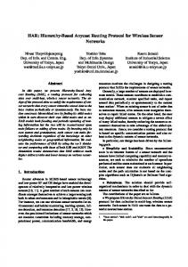
II. A NYCAST ROUTING M ODEL A. Overview In this section, we present our anycast routing model. The model is inspired from field theory in physics. Every group member creates a potential field which decreases with d−k , where d is the distance to the group member, and k determines how quickly the field decreases. The field of an entire anycast group is the linear superposition of all individual fields from the group members. An example field for an anycast group with four members is pictured in Figure 1. The peaks in the field represent the location of the group members. Note that each anycast group has its own field and thus multiple fields co-exist simultaneously. Routing in our model is realized by forwarding packets towards the steepest gradient of the field in analogy to field diffusion in physics. The steepest gradient at a node is determined by comparing the potential value ϕ of its neighbors. The steepest gradient is then the neighbor with the highest potential value. The fundamental difference between the physical field model and our model is that a field in physics is continuous and is propagating in free space whereas in our model, the field is only defined at the network nodes and propagating over the underlying network links. This fundamental difference implies that we can only guarantee the existence of field maxima at group member nodes for ∞ > k > c, where c is a constant we derive in this section. For values of k smaller than c, local maxima may occur and routing along the steepest gradient may not converge. Although, we cannot guarantee routing convergence for that range, we use our model in that range because (i) the occurrence of local maxima in average networks are rare (see Section III) and (ii) local maxima are detected locally (by simply comparing the own potential value with the value of all direct neighbors). Therefore, as soon as a local maximum is detected, an additional mechanism (i.e., switching the routing strategy to shortest path forwarding) could be used at the protocol layer to guarantee routing convergence which is beyond the scope of the model. By varying the shape of the potential field with k, different routing strategies are resulting. We show in this section that a proximity-based routing strategy (the routing strategy of existing anycast routing protocols which consists of forwarding

Potential ϕ

x

y

Fig. 1. Example Potential Field

packets to the closest member along the shortest path) is modeled by setting k > µ, where µ is a constant depending on the network size and the anycast group size. We also show that for 0 < k ≤  (where  < µ), a pure density-based routing strategy is modeled where proximity is no longer considered for routing decisions. By choosing a value for k between µ and , we are able to model combinations of these two routing strategies. Density-based routing is particularly useful for dynamic networks and we therefore also present an extension of the basic model to support dynamic networks. With this extension it is possible to deliver packets successfully even when a node on the steepest gradient fails. B. Potential Fields We define the potential field of an anycast group member j with a strictly decreasing function. That is, the potential value at some node n is defined as: ϕj (n) =

1 dkj (n)

,0 < k < ∞

(1)

where d(n) is defined as the distance of n to the group member j. In this paper, we use the hop count to calculate the distance between nodes. However, the distance could also be calculated using different metrics (such as for example the transmission delay) as long as the potential function remains strictly decreasing. The exponent k in the function determines how quickly the potential decreases with increasing distance to the group member. When there are many members of the same anycast group, the potential field of each group member contributes to the field of the whole group. Thus, the potential field of an anycast group N is defined as the superposition of the potential fields of all members in this group: ϕ(n) =


j∈N

ϕj (n) =


j∈N

1 dkj (n)

(2)

With this definition, the potential field’s shape resembles a landscape with poles at every group member ∀j ∈ N since ϕ → ∞ (in one term of Equation (2) the distance dj (j) is equal to zero hops). By varying the exponent k, the shape of the field varies. For high values of k, the field is steep whereas it is flatter for small values of k.

This full text paper was peer reviewed at the direction of IEEE Communications Society subject matter experts for publication in the Proceedings IEEE Infocom.

C. Gradient-based Routing The previously defined potential field is used to route anycast packets in the network. The routing mechanism is similar to field diffusion in physics. With field diffusion, an element (e.g., a test charge in an electrical field) is always attracted by a force which points in the same direction as the steepest gradient of the field. If the element is free to move, it will diffuse along the steepest gradient until it arrives at a field maximum. In the same manner, we route anycast packets along the steepest gradient of the potential field. The steepest gradient at a node is determined by evaluating the potential values of the node’s neighbors. That is, the link from a node to the neighbor with the highest potential value points to the steepest ascent. Therefore, when a node x receives an anycast packet, it compares the potential value of all its neighbors and forwards the packet to the neighbor with the highest potential value. The potential value of this neighbor must be larger than the potential value of x (note that when there are no local maxima in the field, there always exists a neighbor with a higher potential value as we show later). The node which receives the packet forwards the packet in the same manner until the packet reaches a group member.

there must at least be one neighbor y with a greater potential value: ! (4) ϕ(x) < ϕ(y) We denote N as the set of group members and assume that the distances from x to all group members (di , ∀i ∈ N ) are known. Then we can calculate ϕ(x) and ϕ(y): ϕ(x) =

E. Convergence of Gradient-based Routing Since packets are routed along the steepest ascent, gradientbased routing only converges when there are no local maxima in the potential field. We next derive an upper bound for k depending on the network size and the group size where we can guarantee that no local maxima exist in the potential field. Lemma 2: Consider a connected network with diameter1 D and with an anycast group of size N . The potential function shows no other maxima than at nodes which are group members if k is any constant satisfying: log N (3) D log D−1 Proof: Consider any node x which is not member of the group. To guarantee that the potential value at x is not a maximum,

where N1 , N2 , N3 are disjoint subsets of N (N1 ∪N2 ∪N3 = N and Nu ∩ Nv = ∅, ∀u, v = 1, 2, 3; u = v). The potential value of y must be of this form since x and y are direct neighbors, and the distance of y to any group member can only be one hop smaller, equal, or one hop larger than the distance of x to the corresponding member. Since all terms in Equation (5) are positive by definition, if the potential value at y is still larger than the potential value at x when only considering the contribution from the group members N1 , the potential at node x cannot be a local maximum. Thus, we can simplify the previous condition: ϕ(x) =

that the network diameter D in this paper is defined as the longest shortest path in the network.


1 !
1 < ≤ ϕ(y) k (d − 1)k d i i∈N i i∈N

(6)

1

We even further simplify by only considering at y the potential value from the closest group member s from x: ϕ(x) =


1 ! 1 < k (ds − 1)k d i∈N i

(7)

We now consider the worst case potential value of x. The worst case value is when the potential is maximal. The maximal potential value for x is obtained when the distances to the group members are minimal. Since we said that s is the closest member, ds is the smallest distance that any group member can have. Therefore, the worst case is when all group members are at distance ds : N ! 1 ϕ(x) ≤ k < (8) ds (ds − 1)k We now solve for k and get k>

log N s log dsd−1

(9)

The distance ds is strictly smaller than the network diameter D D s > log D−1 , the condition that the potential and since log dsd−1 value of x is smaller than any neighbor node y is

k>

1 Note

(5)

i∈N3

D. Loop-freeness An important characteristic of a routing algorithm is to provide loop-free routes. We present a sketch of a proof for the following theorem for loop-free routes. Theorem 1: Anycast routing along the steepest ascent in a potential field is loop-free if the network is static. Sketch of Proof: We prove this by showing that a packet cannot traverse a specific node more than once (which is the definition of a loop). Gradient-based routing along the steepest ascent requires that the potential value at every hop on a path is larger than at the previous hop. Since the network is static, the potential value at any node remains constant over time and therefore, it is not possible that a packet traverses one node more than once.



1 !

1 1 < + + k k (di − 1) d dk i∈N i i∈N1 i∈N2 i
1 = ϕ(y) (di + 1)k

k>

log N D log D−1

(10)


We identified the range of k where we can guarantee that there are no local maxima and thus guarantee that routing converges. However, as we will see later, density-based routing strategies require a smaller value of k. Consequently, we also

This full text paper was peer reviewed at the direction of IEEE Communications Society subject matter experts for publication in the Proceedings IEEE Infocom.

ml1 ml2

n2

sender

n1

ms

We assume that ml1 , ..., mln are all equidistant with dl from the sender and we calculate the potential values using Equation (2): ϕ(n1 ) =

mln

ds dl


1 1 1 + > + k k (ds − 1) (dl + 1) (ds + 1)k N −1
1 = ϕ(n2 ) (12) (dl − 1)k N −1

D = dl + ds Fig. 2. Network Topology with one member at distance ds and N −1 members at distance dl > ds

use our model for smaller values of k than the derived bound. When k is smaller than the derived bound, there is no strict guarantee that a packet will reach its destination since local maxima may occur in the potential field. However, we experienced in simulations (see Section III) that this occurs extremely infrequently and we thus also use our model for smaller values of k. F. Effect of Values of k on Routing Strategy The potential field and thus also the resulting routing strategy is selected in our model with the exponent k in Equation (1). By choosing large values of k, the shape of the field is sharp and packets are more attracted towards the close members whereas for small values of k, the shape of the field is flatter and packets are more attracted in the direction of the most group members. In the following, we derive the limit values for k where packets are always routed towards the closest group member along the shortest path and the limit for k where packets are routed only based on the group member density in a specific direction. Lemma 3: Consider a network with diameter D and an anycast group of size N . A packet from any node in the network is always routed to the closest group member of the anycast group along the shortest path, if k is a constant satisfying k > µ(N, D)

(11)

(see Table I for sample values of µ) Proof: We prove this relation by determining the steepest gradient in a worst case scenario and show that it points to the shortest path. The worst case scenario is obtained when all members of a group are located in the opposite direction of the closest group member. This scenario is depicted in Figure 2. The node ms is the closest group member to the sender, however, the remaining N − 1 group members (ml1 , ..., mln ) are all located at the opposite end. This arrangement is the worst case because ml1 , ..., mln create the largest possible potential at node n2 which is in the opposite direction of the closest member, and the smallest possible potential at n1 which is on the shortest path to ms . If we can guarantee that ϕ(n1 ), which is the potential of the node on the shortest path to ms , is larger than ϕ(n2 ), then a packet following the steepest ascent will be forwarded to n1 towards ms on the shortest path. Therefore, the following condition must be met: ϕ(n1 ) > ϕ(n2 )

The worst case for this inequality is obtained when dl is small and ds is large. Therefore, we set the distance dl to the smallest possible distance dl = ds + 1 (which is one hop more than the distance to the closest member ms ) and ds to the largest possible value ds = D−1 2 (since D = ds + dl ) and get 1 N −1 1 N −1 + D−1 > D−1 + D−1 k . (13) k k k ( D−1 − 1) ( + 2) ( + 1) ( 2 2 2 2 ) This equation cannot be solved analytically. We therefore bring it into a cancellation-free form to be able to solve it numerically (see Appendix for further details how we obtained this form): f (k) > N − 1

(14)

with



 D−1 2 −1 log( D−1 ) 2 +1  . · f (k) = D−1 k 1) sinh 2 log( D−12 +2 ) 2 (15) The solution µ for k with sample values of D and N is given in Table I. Since for k > µ, the steepest gradient is always pointing to the shortest path, a packet from any node in the network is always routed along the shortest path.
We now derive the other limit in which a routing strategy always forwards packets towards the highest member density and the distance of a node to group members is irrelevant. Lemma 4: For a network with diameter D and an anycast group of size N , a packet from any node in the network is routed independently of the distances to the members if k is any constant satisfying 

D−1 D−1 2 ( 2 + 2) D−1 ( 2 + 1)( D−1 2 −

 k2

sinh

k 2

0 < k ≤ (D, N )

(16)

log 3 +1 log D−1 D−3

(17)

and N>

(see Table II for sample values of ) Proof: We prove this by calculating the steepest gradient in a best case scenario and show that it does not point towards the next hop on the shortest path of the closest member. We assume again a network topology as depicted in Figure 2 where the closest group member ms is at distance ds from a sender. We determine the smallest factor k when a packet is not routed towards the closest group member independent of how close it is to this member. If a packet is not routed along the shortest path, then the potential value of the next hop towards this member must be smaller or equal to at least one other neighbor: ϕ(n1 ) ≤ ϕ(n2 )

This full text paper was peer reviewed at the direction of IEEE Communications Society subject matter experts for publication in the Proceedings IEEE Infocom.

(18)

D N 4 6 8 10 12 14 16 18 20 22 24

6

8

10

12

14

16

18

20

1.795635 2.936760 3.657162 4.183686 4.598563 4.940854 5.232170 5.485726 5.710183 5.911535 6.094092

2.931176 4.591675 5.652006 6.431778 7.048652 7.559027 7.994312 8.373796 8.710176 9.012257 9.286393

4.049784 6.224987 7.623068 8.654766 9.472706 10.150448 10.729110 11.234018 11.681874 12.084283 12.449630

5.161040 7.849220 9.584353 10.867593 11.886338 12.731245 13.453120 14.083305 14.642505 15.145120 15.601562

6.268394 9.468746 11.540646 13.075283 14.294741 15.306746 16.171770 16.927177 17.597668 18.200436 18.747926

7.373423 11.085512 13.494042 15.280017 16.700152 17.879221 18.887369 19.767971 20.549730 21.252628 21.891138

8.476947 12.700515 15.445605 17.482893 19.103687 20.449810 21.601069 22.606854 23.499864 24.302877 25.032397

9.579444 14.314324 17.395938 19.684523 21.505970 23.019141 24.313505 25.444466 26.448721 27.351841 28.172357

TABLE I S AMPLE VALUES OF µ. N IS THE NUMBER OF ANYCAST GROUP MEMBERS AND D IS THE NETWORK DIAMETER .

or



1 1 1 1 + ≤ + . k k k (ds − 1) (dl + 1) (ds + 1) (dl − 1)k N −1 N −1 (19) In the best case, ms is very close to the sender and all other group members are far away. Therefore, we set ds to the smallest possible value ds = 2 and dl to the largest possible value dl = D − ds = D − 2 (Note that we do not consider the trivial case ds = 1 since then a packet will always be routed to ms because it is now a direct neighbor of ms with a potential of ϕ → ∞). Now we get: 1+

1 N −1 N −1 ≤ k + . k (D − 1) 3 (D − 3)k

(20)

This inequality cannot be solved analytically and we therefore bring it in a cancellation-free form to solve it numerically (see Appendix for further details): f (k) ≤ N − 1 with 

(D − 1)(D − 3) 3

k/2

  sinh k2 log 3  . · sinh k2 log( D−1 D−3 )

Note that this inequality has solutions only for N −1 >

(21)

(22) log 3 log D−1 D−3

.

The solution  of this inequality is given for sample values of D and N in Table II. Since for k ≤ , the steepest gradient does not correlate with the shortest path, packets are routed independently of the distance to the members.
We finally consider the special case where the group size is equal to one. Lemma 5: For a network with group size N = 1, a packet is always routed along the shortest path to this member independent of k. Sketch of Proof: If the anycast group size is equal to one, the potential values of each node is inverse proportional to the distance of the member. Therefore, by forwarding a packet along the steepest gradient, a packet is forwarded over the shortest distance.


G. Extension for Dynamic Networks So far, we have shown the properties of potential field based routing. However, this routing technique is particularly interesting when network topologies are dynamic and nodes are mobile. We therefore propose a simple extension of the model to support dynamic networks where we loose the requirement of constantly keeping precise potential field values up-to-date. The approach is based on the observation that in dynamic networks, some neighbors and links might disappear but the remaining links and the potential field information still contains fresh enough routing information to route the packet towards the destination. When a node wants to forward a packet and the link with the steepest gradient of the potential field becomes unavailable, we do not have to re-calculate the entire potential field in the network. We simply forward the packet to the neighbor with the next highest potential value. The advantage of this approach is that this neighbor is determined locally by the node that detects the link failure. The routing table contains enough redundant routing information to perform some kind of ”local repair”. Therefore, when implementing our model in a protocol, this approach will provide much better performance with a reduced overhead. This extension of the model still avoids routing loops since the potential value at each hop must increase, which is not possible in a loop. However, this extension does not guarantee anymore that a packet will reach a group member. At the end of the next section, we measure the packet delivery ratio of this extension for dynamic networks. III. M ODEL E VALUATION In this section, we evaluate our model using extensive simulations of wireless networks. We study the effect of different values of k on the potential field and the resulting anycast forwarding strategies. We also analyze the occurrence of local maxima in the potential field and show that for random networks, local maxima only form very rarely. Finally, we evaluate the convergence of field-based routing for dynamic networks where the nodes are mobile.

This full text paper was peer reviewed at the direction of IEEE Communications Society subject matter experts for publication in the Proceedings IEEE Infocom.

D N 6 8 10 12 14 16 18 20 22 24

6

8

10

12

14

16

18

20

0.129472 0.343468 0.511681 0.650004 0.767310 0.869051 0.958808 1.039066 1.111609

0.061210 0.197150 0.309386 0.404871 0.487902 0.561315 0.627080 0.686620

0.031419 0.129192 0.212506 0.285049 0.349261 0.406841 0.459017

0.015418 0.090838 0.156559 0.214772 0.267005 0.314358

0.005733 0.066601 0.120540 0.168956 0.212865

0.050101 0.095628 0.136930

0.038259 0.077500

0.029415

TABLE II S AMPLE VALUES OF
. N IS THE NUMBER OF ANYCAST GROUP MEMBERS AND D IS THE NETWORK DIAMETER .

Ratio of nodes with changed steepest gradient

Ratio of nodes with changed steepest gradient

A. Effects of Values of k on Potential Fields In the previous section, we identified upper bounds for k when the anycast routing strategy always finds the shortest path 0.7 15 members and strategies where the member distance has no effect on packet 10 members 0.6 delivery. In the following, we study the routing behavior of 5 members 3 members routing strategies with values of k between these two extreme 0.5 2 members cases. 1 member To determine the effect of different values of k on the steepest 0.4 gradient of the potential field, we do the following. We calcu0.3 late the potential field for a network with a very high value of k (in this case k = 1000) as a reference field. This high value 0.2 guarantees that the resulting steepest gradient is pointing to the next hop along the shortest path to the closest member at every 0.1 node (see Section II). Then, we calculate the potential field of 0 different values of k for the same network topology and com1000 100 10 1 0.1 0.01 0.001 1e-04 1e-05 pare these with the reference field. We define the metric for the k difference of two fields as the number of nodes at which the direction of the steepest gradient has changed. For example, a (a) diameter D=18 difference of 0.5 means that at 50% of the nodes, the neighbor with the highest potential value is not identical compared to the node of the reference field. Note that since the distance metric 0.7 indicates how often the steepest gradient changes in a field, it 10 members also captures the effect of changes in the routing strategy be5 members 0.6 3 members cause packets are routed along the steepest gradient. 2 members In the following, we plot the difference of the reference field 0.5 1 member with fields obtained with various k. The plots are obtained by 0.4 averaging the result of random wireless networks, which were generated as follows. A fixed number of nodes are randomly 0.3 placed on a quadratic plane (2000m x 2000m). There exists a bidirectional link between two nodes if their geometric dis0.2 tance is less than or equal to the wireless range (a fixed value identical for all nodes). This model corresponds to a flat envi0.1 ronment with devices equipped with wireless radio, all having 0 equal communication range. The anycast group members are 1000 100 10 1 0.1 0.01 0.001 1e-04 1e-05 assigned randomly to the existing nodes. k In Figure 3(a), we used a network size of 400 nodes and set the wireless radio range to 200m in order to obtain a connected (b) diameter D=13 (every node can reach any other node) network. All networks had a network diameter size of D = 18 and the average node degree was approximately 12. Group sizes between 1 and 15 Fig. 3. Effect of k on the steepest gradient members were used. For the different group sizes, we plot the

This full text paper was peer reviewed at the direction of IEEE Communications Society subject matter experts for publication in the Proceedings IEEE Infocom.

Ratio of nodes with changed steepest gradient

0.8 0.7 0.6

0.5

node degree = 14.27 node degree = 12.88 node degree = 10.03 node degree = 7.22 node degree = 6.23

0.4

I

II

III

IV

0.3

0.5 0.2

0.4 0.3

0.1

0.2 0

0.1 0 1000 100

1000

10

1

0.1 k

100

10

1

0.1 k

0.01

0.001

1e−04

1e−05

0.01 0.001 1e-04 1e-05 Fig. 5. Four Categories of Strategies (curve for D=18, N=15)

Fig. 4. Effect of k on the steepest gradient

Category ratio of nodes affected by changes in the field on the vertical axis for values of k between 1000 and 1e−5 . For all group sizes, the potential field differs from the reference field for values of k below approximately 200. When k becomes smaller than approximately 0.01, reducing k does not further produces any change in the field. We also observe that the difference between the reference field is bigger for larger groups. For a group size of 15 members, the steepest gradient changes at more than 40% of the nodes. Note that the steepest gradient is not affected by k for a group size of one member. In that case, the potential field always results in a shortest path routing strategy for all values of k as proved in Section II. In Figure 3(b), we reduced the number of nodes to 200 and increased the wireless range to 280m to still obtain connected networks. All networks were of diameter D = 13 and the average node degree was approximately 12 as in the previous plot. The resulting plot is similar to Figure 3(a). The gradient changes occur at similar values of k for the respective group sizes. For small values of k however, the total field difference is smaller We also investigated the effect of k on the field for different network densities. In Figure 4, the difference is plotted for different network densities and a fixed group size of N = 10. Different network densities were obtained by varying the number of nodes from 220 to 500 while keeping the wireless range of each device to 200m. We measure the network density as the node degree averaged over all nodes. As the plot shows, the potential field is subject to more changes when the network density is high. This is due to the fact that the denser the network is, the more paths are available. B. Effects of Values of k on the Routing Strategy The shape of the curves in Figure 3 and 4 show clear patterns and we use them to classify the routing strategies into different categories. In the following, we define four main categories (I IV) of routing strategies and explain their properties. We know from Section II that for very large values of k, packets are routed to the closest member without considering the member density in any specific direction. Therefore, if we

I II III IV

proximity based routing yes yes yes no

density based routing no yes yes yes

Delivery to closest member over shortest path yes yes no no

TABLE III ROUTING C ATEGORIES AND THEIR P ROPERTIES

look at the field difference curve from Figure 5 (this example curve was obtained with D=18 and N=15), we classify all routing strategies with zero difference compared to the reference field, as strategies that only consider the closest group member for routing decisions. We marked these strategies with category I in the figure. Note that the existing anycast routing protocols ([7], [10], [11], [12], [13]) all employ this proximity-based routing strategy. For k smaller than approximately 200 in the figure, the influence of density starts to act since the difference to the reference field is greater than zero. However, this shift in the steepest gradient does not impact the delivery path length since we know from the previous section that even in the worst case, in a network with diameter D=18 and group size N=15 as used in the example, any strategy with a value of approximately k > 20 still forwards over a shortest route. What happens in this case is that when different members are equidistant and closest to a node, the member which in the direction of the highest member density is preferred. We define this range as a separate category (category II) of routing strategies, where packets are still routed to one of the closest member over the shortest path but where density is considered at the same time. We will see later in this section the benefits of category II versus category I in terms of robustness. By further decreasing k, the effect of density-based routing outweighs more and more the effect of proximity-based routing in the routing strategy. At a certain point, packets start to travel over paths which are no longer the shortest ones. As soon as one delivery path in the network is no longer the shortest, we declare the routing strategy to belong to the category III.

This full text paper was peer reviewed at the direction of IEEE Communications Society subject matter experts for publication in the Proceedings IEEE Infocom.

Node Probability of Local Maximum

100

k

10

1 worst case (D=18) worst case (D=13) average case (D=18) average case (D=13) 2

4

6

8

10

12 N

14

16

18

20

Fig. 6. Transition between category II and III. The value of k indicates the smallest allowed value that still results in shortest path forwarding. The worst case is the derived upper bound, and the average case is an empirical value obtained with simulations.

Thus, in this category, routing decisions are based on a tradeoff between member distance and member concentration, but in contrast to category II, packets are no longer delivered over the shortest paths to the closest member. For very small values of k (smaller than 0.001 in the example), the plot shows that the potential field no longer changes when decreasing k. Therefore, we define category IV at this point. With category IV, routing decisions are only based on the member concentration and the member distance is no longer relevant. Note that the limit between phase III and phase IV is not as sharp as indicated in the figure. The limit could be as well more to the left or to the right side. To summarize, the four categories and their properties are listed in Table III. To highlight the transition line between category II and III, we plot the transition value of k between these two categories versus the group size N in a separate plot in Figure 6. Recall that the difference between category II and III is that packets in category III are no longer routed over the shortest path, which is still the case in category II. Thus, this value is the smallest possible value of k until routing is still following the shortest path. For completeness, we also plot the worst case value µ obtained in the previous section. We find that the values obtained with the simulations (denoted with average case values) on random networks with D = 13 and D = 18 are between 4 > k > 1. The worst case values are quite close to the average values for small group sizes and tend to be significantly larger for group sizes around 20 members. C. Local Maxima Local maxima in the potential field might occur in our model since the potential is a discrete function only defined at the network nodes and the field propagation is constrained to the physical links of the underlying network. We have seen in the previous section that we can guarantee that there are no local maxlog N ima in a field with k > log D . However, since we also use D−1

our model for smaller values of k, we have to investigate how

N=25 N=15 N=10 N=5 N=3 N=2

0.00015

0.0001

5e-05

0 1000 100

10

1

0.1 0.01 0.001 1e-04 1e-05 k

Fig. 7. Local Maximum Likelihood vs. k

Node Probability of Local Maximum

0.1

0.0002

0.00012

k=0.001 k=0.01 k=0.1

0.0001 8e-05 6e-05 4e-05 2e-05 0 0

5

10 15 Group Size N

20

25

Fig. 8. Local Maximum Likelihood vs. Group Size N

frequent local maxima are. In this section, we show with simulations of random networks that the occurrence of local maxima is low for different values of k, for different group sizes, and different network densities. Figure 7 shows the probability that a non-member node becomes a local maximum for values of k between 1000 and 10−5 . Note that the resulting curves are obtained by averaging at least two thousand random networks with 500 nodes. The average node degree in those networks is approximately 12. The plot shows that for large values of k (k > 3), there are no local maxima in the potential field independent of the group size. For k < 3, some very few local maxima form. However, the probability remains quite low. In this specific case, the probability is always below 0.01% for the used group sizes. We also plot the probability of local maxima versus the group size on the horizontal axis in Figure 8. For group sizes of 2 and below, there are no local maxima. Local maxima start to happen from a group size of 3. Note, that the highest probability for a local maximum is reached with a group size of 5. For larger groups, the probability decreases significantly. This is mainly because local maxima form only in specific star topologies, when the group members are in different directions but

This full text paper was peer reviewed at the direction of IEEE Communications Society subject matter experts for publication in the Proceedings IEEE Infocom.

1

k=0.001 k=0.01 k=0.1 k=0.6 k=3

0.0002

Packet Delivery Ratio

Node Probability of Local Maximum

0.00025

0.00015 0.0001 5e-05

0.8 0.6 0.4 k = 0.01 k = 0.1 k=3 k = 50 k =300

0.2

0

0 6

8

10

12 14 16 Node Degree

18

20

22

0

0.05

0.1 0.15 0.2 Ratio of Broken links

0.25

0.3

Fig. 9. Local Maximum Likelihood vs. Network Density

Fig. 10. Routing Convergence with Network Dynamics

about the same distance from a node. By increasing the group size, the probability that such a topology occurs, decreases. In Figure 9, the occurrence of local maxima is plotted for different network densities. We express the network density with the average node degree of the nodes on the horizontal axis. We obtained networks of different average node degrees (densities) by varying the number of nodes while keeping the simulation area size constant. For the smallest average node degree of 7.8, the number of nodes was 250 and for the largest average node degree of 20.5, the number of nodes was 700. We observe a higher probability for local maxima in low density networks. For example, with k = 0.1, the probability of a local maximum at a node is 0.018% for a node degree of 7.8. However, by increasing the node degree to 20.5, the probability is only 0.0027%. This result confirms our expectation. By increasing the node density in our model, the discrete field approaches a continuous field without any constraints in the propagation space (which does not show local maxima). As previously mentioned, for k ≥ 3, there are no local maxima in the field.

using a link connectivity model [14] which consists of removing random links from the network using a uniform distribution. Note that the potential field is not adapted after the links become unavailable. We send packets from random sources and count the number of packets that arrive at group members. Packets are dropped when a node has no longer a neighbor with a higher potential value than itself. The packet delivery ratio for this experiment is plotted in Figure 10. On the horizontal axis, we plot the ratio of broken links which indicates the degree of network dynamics or network stability. A value of 0.1 means that 10% of the existing links in the original network topology are unavailable. We observe that when the ratio of broken links is zero, the packet delivery ratio is 100% for all anycast routing strategies. When the ratio of broken links increases, the packet delivery ratio is better for small values of k (i.e., packets are routed based on member density). For example, when 30% of all links are broken, still 80% of the packets are delivered for k < 3 whereas only 66% of the packets are delivered for k = 50 and 53% of the packets for k = 300. Notice that the packet delivery ratio in this scenario is roughly the same for k = 3, k = 0.1, and k = 0.01. This is an interesting result since for k = 3, the routing strategy is in phase II, which means that packets are still forwarded over the shortest path. That is, with k = 3 in static networks, we will always forward packets over the shortest path. In dynamic networks, the density-based routing however, increases the packet delivery rate by 23% compared to pure (k = 300) proximity-based routing strategies.

D. Routing with Network Dynamics So far, we evaluated our model for static networks. Now, we look at the routing convergence when the network is dynamic. When the network is dynamic, the link to the node on the steepest gradient might become unavailable (e.g., when a node moves away) and the potential field remains outdated for a limited period of time until the correct potential field is recalculated. In these situations, we proposed to route the packet to the neighbor with the next highest potential value. However, since the next best neighbor is not along the original steepest gradient, there is no strict guarantee that a packet reaches an anycast group member. To evaluate this effect, we measure the resilience to link failures for different routing strategies. Resilience is determined by the packet delivery ratio (the total number of packets received by group members to the total number of packets sent). We generate random networks (in the same way as in previous scenarios) with 500 nodes from which ten are group members. For each network, we calculate the potential field on the initial topology and then simulate mobility

IV. S CENARIO - BASED E VALUATION So far, we evaluated the behavior and performance of the routing strategies in stable and dynamic networks. To better understand the advantages of the density-based routing strategy, we apply our model to examine different anycast strategies for specific types of dynamic networks, specifically, mobile sensor networks. For this evaluation, we developed our own network simulator.

This full text paper was peer reviewed at the direction of IEEE Communications Society subject matter experts for publication in the Proceedings IEEE Infocom.

A. Scenario Description of Sensor Data Collection

B. Communication and Network Model We model communication and node mobility in the following way. At time t0 , the potential field is instantaneously created in the network and a random sensor node generates a data packet which is sent via anycast to the neighbor following the steepest ascent of the potential field. The receiving node caches the data packet for a time period δt before forwarding the packet. After δt, the potential field is recalculated at each node according to the new network topology (if nodes moved within the delay time δt) and the packet is then forwarded again towards the steepest ascent. This procedure is repeated until the packet arrives at a data sink. Note that with this procedure, even if the nodes are mobile, the potential field is always correct when a packet is forwarded. In practice, it would require that the control messages to establish the potential fields have been sent right before the packet is sent. Although not completely realistic, this idealized scheme allows us to study the performance of the different anycast routing strategies separately without accounting for the inaccuracy of an underlying protocol used to establish the respective routing tables. Also, this idealized scheme guarantees that, unless there are local maxima in the potential field, data packets will reach a data sink. Note that for fairness in the comparison of the different strategies (some strategies have more local maxima than others as we have seen in previous evaluation), we did not account for simulations in which local maxima occurred. As discussed before, local max-

2.4 2.2 2 Ranking

Sensor networks are used to collect environmental data from sensors. A typical sensor network consists of small, autonomous, battery-powered sensor nodes connected via radio links. The data collected by these sensors is then transmitted over multiple hops to the closest data sink for further processing or analysis. Since sensors can send their data to any of the data sink nodes, anycast is a convenient delivery mode for this type of scenario. Sensor networks often have hard energy and resource constraints due to the limitation of the sensor nodes but, on the other hand, they are more delay tolerant than traditional data networks. As a consequence, sensor networks employ extensive usage of sleep operations and caching. Therefore, packets from sensors are often delayed in the network until they arrive at the destination and the end-to-end delay can thus be in the order of seconds or even minutes compared to milliseconds if it would have been sent directly. Due to the increased end-to-end delays, it is likely that nodes move and the network topology changes during the data delivery. In this section, we analyze the efficiency of different anycast delivery strategies in scenarios where the topology changes occur during ongoing transmissions. We do so by analyzing the delivery path length of different anycast routing strategies which we instantiate with our model by selecting specific values for k. We consider sensor networks with three different mobility patterns. In the first scenario, the sensors as well as the data sinks are mobile. In the second scenario, the sensors are mobile but, the data sinks are at fixed locations. In the third scenario, the sensors are fixed and the data is collected by mobile data sinks.

1.8 1.6 k = 300 k = 50 k=3 k = 0.1 k = 0.01

1.4 1.2 1 0

200

400

600

800

1000

v · δt [m] Fig. 11. Traversed Path Length with Moving Sensors and Data Sinks

ima appear only very rarely (in less than 0.1% of all simulations). In spite of the known limitations[15], we use the random waypoint model [16] as the mobility model. 500 nodes move around in a quadratic area with a side length of 2000 m. With the random waypoint model, each node chooses a random destination and moves towards this destination on a straight line with a constant speed v. In this model, a node stops moving for a constant pause time p when it arrives at its destination. We set this pause time to p = 0s which means that the nodes are constantly moving in the simulations. Ten of the 500 nodes are data sinks belonging to the same anycast group. The remaining nodes are all sensor nodes. The wireless range of the radio device at each node is set to 180 meters. There exists a link between two devices if their geometric distance is smaller than the wireless range. We chose the above parameters so that the network remains connected during the total simulations and we do not have to account for the case where nodes are within a cluster, unable to access any data sink. We do not model the behavior of any MAC or physical layer characteristics in the simulations as we are only interested in the traversed path length of data packets. C. Results We investigated the path length traversed by packets for the different anycast routing strategies. In Figure 11, the results are plotted for the first scenario where all nodes are mobile. The horizontal axis of the plot indicates the node speed multiplied with the forwarding delay δt. This factor is an indicator of how much the network topology changes between each forwarding step. The metric indicates the distance covered by a node and is measured in meters. On the vertical axis, the ranking of the different routing strategies is plotted. The ranking is an averaged value over all simulation runs. For example, if an anycast forwarding strategy has a ranking of 1, it means that the packets delivered with this strategy were delivered over shorter paths than the other strategies in all simulation runs. Note that we chose to plot a ranking of the strategies instead of the average path length because few paths happened to be

This full text paper was peer reviewed at the direction of IEEE Communications Society subject matter experts for publication in the Proceedings IEEE Infocom.

2.4

2.2

2.2

2

2 Ranking

Ranking

2.4

1.8 1.6 k = 300 k = 50 k=3 k = 0.1 k = 0.01

1.4 1.2 1 0

200

400

600

800

1.8 1.6 k = 300 k = 50 k=3 k = 0.1 k = 0.01

1.4 1.2 1 1000

v · δt [m]

0

200

400

600

800

1000

v · δt [m]

Fig. 12. Traversed Path Length with Fixed Data Sinks and Mobile Sensors

Fig. 13. Traversed Path Length with Fixed Sensors and Mobile Data Sinks

a lot larger compared to the remaining ones which makes an average value of different runs somewhat unfair. We find that when the node speed or the forwarding delay is zero (0m on the horizontal axis), forwarding strategies with a larger value of k (strategies which favors proximity) tend to find shorter paths than strategies with small values. More precisely, strategies with k = 300, 50, and 3 always find shorter paths than strategies with k = 0.1 and 0.01. When the speed-delay product is increased, we see that the performance of k = 300 quickly decreases compared to the strategies with k = 50 and k = 3. At a speed-delay product of 100m (e.g. v = 10m/s and δt = 10s), the average ranking for k = 0.1 is even equal to the strategy with k = 300. At a speed-delay product of 280m, the strategies with k = 0.1 and k = 0.01 even find shorter paths than all other strategies which were better in the static case. When the speed-delay product becomes too large (1000m), the topology between two transmissions is so different that the strategy has no more any effect on the performance. In the next scenario (see Figure 12), we did the same experiment while maintaining the data sinks at a fixed (random) location. For the speed-delay product between 0 and 200, the trend is similar to the previous experiment in which all nodes were mobile. However, we assess that for speed-delay products larger than 200, strategies with small k (in this case k = 0.1 and 0.01), tend to find shorter paths. Even when the speed-delay factor is 1000, these strategies perform better than the others. We also analyzed the effect of k in scenarios where the sensor nodes are all at a fixed location and the data collecting devices are moving. In this set of scenarios, the strategies with a small values of k take longer to outperform the others. However, for a speed-delay product beyond 300, the strategies outperform the others much more clearly (approximately a ranking of 1.4 for k = 0.1 and 0.01). Note that for this scenario, the ranking of a pure proximity-based strategy with k = 300 is much worse compared to combined strategies with k = 50 and k = 3.

the best of our knowledge, this is the first paper to propose an alternative routing strategy for anycast. Routing based on potentials has been proposed previously. In [17], routing using potential fields was first proposed for unicast routing in the Internet. Since the authors aimed at developing a unicast routing algorithm, the potential field in this work has only one maximum value at the target destination, which makes convergence much easier to achieve. In [18], [25], the usage of potential fields was proposed for service discovery in mobile ad hoc networks. In this work, the potential field is inspired by the electrical potential field that is defined for a service as ϕj (n) = djQ(n) where Q is a positive charge modeling the capacity of the service. Therefore, the specific field used in this work can be instantiated with our model by choosing k = 1 (k is the exponent in Equation 1) and setting Q = 1. The main difference from this work is that we consider potential fields for 0 < k < ∞ and not just k = 1. IP anycast was originally proposed in 1993 for IPv4 [1]. Later, it was incorporated into the IPv6 addressing architecture [19]. The reasons why IP anycast is not widely deployed nowadays in the Internet is mainly due to two problems. IP anycast, as originally proposed, does not scale well and it is hard to deploy at a large scale. For the first problem, Katabi et. al. proposed GIA [20] as a scalable IP architecture. Recent ideas to make IP anycast more easily deployable were proposed in [21] and [22]. Although scalability and ease of deployment are fundamental to the success of anycast in the Internet, it is less important for infrastructure-less or self-organized networks such as mobile, ad hoc networks, or sensor networks which is where we plan to make use of our approach. We expect these kind of networks to be smaller (hundred to thousands of nodes compared to millions of nodes in the Internet) and to be used for “local” communication (e.g. for communication within a city or a group of persons). Furthermore, self-organizing networks often do not rely on an existing routing infrastructure, which makes the problem of protocol deployment much easier. Vincent Park et. al. described in [7] and [23] how to extend known unicast routing techniques such as link state, distance vector, and link reversal routing for anycast delivery. However, by extending unicast routing techniques, is is only possible to

V. R ELATED W ORK This paper proposes density-based anycast routing, an alternative anycast routing strategy to proximity-based routing. To

This full text paper was peer reviewed at the direction of IEEE Communications Society subject matter experts for publication in the Proceedings IEEE Infocom.

build anycast routing protocols which find the shortest route to the closest group member. Jianxin Wang et al. proposed in [10] and [12] to extend AODV [24] and DSR [16] respectively to support anycast delivery in mobile ad hoc networks. These protocols can be instantiated with our model by choosing a large value of k. The main drawback of these protocols is again that they only consider the closest group member when computing routes.

with the most anycast group members. Later, packet routing converges to shortest path routing and the packet ”selects” a unique destination (the closest group member). In a first step however, we have to investigate if routing still converges under these conditions.

We have shown that the routing strategy is defined by the value of k. The optimal value for k depends on the characteristics of the concerned network and the anycast application. Hence, the network designer or operator can set k to best fit the expected network characteristics. On the other hand, since every node calculates its potential value independently of other nodes, an interesting alternative is to let the sender decide with which value of k its packets should be routed. In that way, the sender or the sending application controls the routing strategy for its packets by assigning the value of k set in the packet header. Note that this mechanism offers, to some extent, source routing-like control without the overhead of route determination in advance. In the sensor network scenario described in Section IV, a node would assign a packet with a large k when the network topology is stable and send packets with a lower k for more network dynamics. Another alternative mechanism that we plan to study in future work, is to adapt the value of k in a packet as it propagates in the network. For example, a packet is originally sent with a low value of k at the sender. As the packet traverses the network the value of k increases at each hop. This implementation dynamically change the routing strategy as a packet is routed. At the beginning, the packet is routed to the network region

ACKNOWLEDGMENTS

VII. C ONCLUSIONS

In this paper, we have examined the existing anycast routing strategies and introduced a new family of anycast routing VI. D ISCUSSION AND I MPLEMENTATION I SSUES schemes: density-based routing. We presented a model that Given that our model provides an easy way to instantiate represents both, the existing anycast routing schemes as well as proximity- and density-based routing strategies, we consider in the density-based ones. We have shown that the schemes prothis section two fundamental issues required to implement the vide loop-free routes and studied the properties of the routing model as a protocol. strategy. We use the results from the model evaluation to categorize the routing strategies into four types: (I) proximity-based routing; (II) proximity-based routing considering density; (III) A. Calculating the Distance to the Group Members routing as the tradeoff between proximity and density; and (IV) Our model requires every node to calculate its potential value pure density-based routing. according to Equation 2. Therefore, every node must know Our results show that our routing model is of particular inits distance to every group member. There are two basic apterest in dynamic networks. In these networks, a density-based proaches to obtain these distances: (i) the group members send algorithm achieves a 23% performance improvement compared periodic advertisements containing distance information (for exto pure proximity-based approaches. We also evaluated our ample, the number of traversed hops); or (ii) the routers actively routing strategy in a given sensor scenario. We have shown query the network with probe packets and the anycast group that in the sensor networking environments we studied, densitymembers then reply when they receive the query. Since the based routing clearly outperforms standard proximity-based routgroup size is usually smaller than the total number of nodes/routers, ing approaches. We even show that in highly dynamic netit is more efficient to let the group members periodically adworks, a density-based routing strategy produces shorter path vertise themselves. Indeed, approach (i) has been successfully lengths than pure proximity-based routing schemes. implemented in [18], [25]. In this work, we presented a protoDensity-based routing schemes offer many opportunities for col that maintains the potential fields up-to-date with moderate future research. For example, adapting the routing strategy as control overhead for highly dynamic networks were nodes are packets are forwarded. Another open issue is how to implement moving with speeds up to 20 m/s. an efficient protocol to disseminate potential information when the network is dynamic or even disrupted. B. Choosing k We would like to thank J¨org Waldvogel and Ulrich Fiedler for their help on the mathematical aspects of the paper. We also thank all the anonymous reviewers who helped improving the paper in many ways. R EFERENCES [1] C. Partidge, T. Mendez, and W. Milliken, “Host Anycasting Service,” IETF RFC 1546, November 1993. [2] T. Hardie, “Distributing Authoritative Name Servers via Shared Unicast Addresses,” RFC 3258, April 2002. [3] D. Kim, D. Meyer, H. Kilmer, and D. Farinacci, “Anycast Rendevous Point (RP) mechanism using Protocol Independent Multicast (PIM) and Multicast Source Discovery Protocol (MSDP),” RFC 3446, January 2003. [4] Sylvia Ratnasamy, Scott Shenker, and Steven McCanne, “Towards an Evolvable Internet Architecture,” in SIGCOMM, Philadelphia, USA, August 2005. [5] C. Huitema, “An Anycast Prefix for 6to4 Relay Routers,” RFC 3068, June 2001. [6] J. Moy, “OSPF Version 2,” IETF RFC 2328, April 1998. [7] V. Park and J. Macker, “Anycast Routing for Mobile Services,” in Conference on Information Sciences and Systems (CISS), Baltimore, MD, USA, March 1999. [8] G. Malkin, “Rip version 2,” IETF RFC 2453, November 1998. [9] V. Park and S. Corson, Temporally-Ordered Routing Algorithm (TORA), IETF Internet Draft, July 2001.

This full text paper was peer reviewed at the direction of IEEE Communications Society subject matter experts for publication in the Proceedings IEEE Infocom.

[10] Jianxin Wang, Yuan Zheng, and Weijia Jia, “An AODV-based Anycast Protocol in Mobile Ad Hoc Network,” in Proc. of the IEEE International Symposium on Personal, Indoor and Mobile Radio Communication, Beijing, China, September 2003. [11] Chalermek Intanagonwiwat and Dante De Lucia, “The Sink-Based Anycast Routing Protocol for Ad Hoc Wireless Sensor Networks,” Tech. Rep. 99-698, USC Computer Science, CA, USA, 1999. [12] Jianxin Wang, Yuan Zheng, and Weijia Jia, “A-DSR: A DSR-based Anycast Protocol for IPv6 Flow In Mobile Ad Hoc Networks,” in Proc. of the IEEE Vehicular Technology Conference, Orlando, Florida, USA, October 2003. [13] Ulas C. Kozat and Leandros Tassiulas, “Network Layer Support for Service Discovery in Mobile Ad Hoc Networks,” in Proceedings of the IEEE INFOCOM, San Francisco, USA, April 2003. [14] T. Lin, S. F. Midkiff, and J. S. Park, “Mobility versus Link Stability in Simulation of Mobile Ad Hoc Networks,” in Proceedings of Communication Networks and Distributed Systems Modeling and Simulation Conference, 2003, pp. 3–8. [15] Christian Bettstetter, Giovanni Resta, and Paolo Santi, “The Node Distribution of the Random Waypoint Mobility Model for Wireless Ad Hoc Networks,” IEEE Transactions on Mobile Computing, vol. 2, no. 3, pp. 257–269, 2003. [16] David B. Johnson, David A. Maltz, Yih-Chun Hu, and Jorjeta G. Jetcheva, “The Dynamic Source Routing Protocol for Mobile Ad Hoc Networks (DSR),” February 2002. [17] Anindya Basu, Alvin Lin, and Sharad Ramanathan, “Routing Using Potentials: A Dynamic Traffic-Aware Routing Algorithm,” in Proceedings of the ACM annual conference of the Special Interest Group on Data Communication (SIGCOMM’03), Karlsruhe, Germany, August 2003. [18] Vincent Lenders, Martin May, and Bernhard Plattner, “Service Discovery in Mobile Ad Hoc Networks: A Field Theoretic Approach,” in Proceedings of the IEEE International Symposium on a World of Wireless, Mobile and Multimedia Networks (WoWMoM), Taormina, Italy, June 2005. [19] S. Deering and R. Hinden, “IP Version 6 Addressing Architecture,” IETF RFC 2373, July 1998. [20] Dina Katabi and John Wroclawski, “A Framework for Scalable Global IP-Anycast (GIA),” in Proc. of ACM SIGCOMM, Stockholm, Sweden, August 2000. [21] Ion Stoica, Daniel Adkins, Shelley Zhuang, Scott Shenker, and Sonesh Surana, “Internet Indirection Infrastructure,” in Proceedings of ACM SIGCOMM Conference, Pittsburgh, PA, USA, August 2002. [22] Hitesh Ballani and Paul Francis, “Towards a Global IP Anycast Service,” in Proc. of ACM SIGCOMM, Philadelphia, USA, August 2005. [23] Vincent D. Park and Joseph P. Macker, “Anycast Routing for Mobile Networking,” in Proc. of MILCOM, Atlantic City, New Jersey, USA, November 1999. [24] Charles E. Perkins, Elizabeth M. Belding-Royer, and Samir R. Das, “Ad Hoc On-Demand Distance Vector (AODV) Routing,” IETF Internet Draft, draft-ietf-manet-aodv-12.txt, November 2002. [25] Vincent Lenders, Martin May, and Bernhard Plattner, “Service Discovery in Mobile Ad Hoc Networks: A Field Theoretic Approach,” Elsevier Journal on Pervasive and Mobile Computing, vol. 1, no. 3, September 2005.

2

2

This inequality cannot be solved analytically for k. Before solving it numerically, we have to bring it in a cancellation-free form where the terms do not cancel each other. Therefore, we first separate k and N :

(27) In this form, it is now possible to find numerically the solution for f (k) > N − 1 (e.g., using the secant method). B. Extension for Proof of Lemma 5 The condition that the steepest gradient does not point to next hop on the shortest path is: 1+

1 N −1 N −1 ≤ k + k (D − 1) 3 (D − 3)k

(28)

Again, this inequality cannot be solved analytically for k, and solving it numerically is problematic since the form is not cancellationfree. Therefore, we bring it to a form where the terms do not cancel each other. We first separate k and N : N −1≥

1 − 31k = f (k) 1 1 − (D−1) k (D−3)k

(29)

The function f (k) can be written as: f (k) =

1−k − 3−k (D − 3)−k − (D − 1)−k

(30)

k

By using the relationship a−k − b−k = 2(ab)− 2 sinh( k2 log ab ), we get

= f (k)

(24)

D−1 D−3 )

−k −k − ( D−1 ( D−1 2 + 1) 2 − 1) −k − ( D−1 )−k ( D−1 2 + 2) 2

(31)

or f (k) =

 (D − 1)(D − 3)  k2 3

sinh( k2 log 3) sinh( k2 log

D−1 D−3 )

√

(32)

It can be shown that for D > 1+2 13 ≈ 2.3, f (k) is monotonously increasing for any k > 0. With this restriction for D, which means that the network diameter must at least be 3, N − 1 ≥ f (k) has valid solutions if N − 1 > loglog D3 . The solutions can D−1

again be found with e.g. the secant method.

The function f (k) can also be written as: f (k) =

+2

k

1 N −1 1 N −1 + D−1 > D−1 + D−1 k (23) k k k ( D−1 − 1) ( + 2) ( + 1) ( 2 2 2 2 )

N −1