Density Evolution for Asymmetric Memoryless Channels - CiteSeerX

1

Density Evolution for Asymmetric Memoryless Channels: the Perfect Projection Condition and the Typicality of the Linear LDPC Code Ensemble

Chih-Chun Wang, Sanjeev R. Kulkarni, H. Vincent Poor

This work was supported in part by the National Science Foundation under Grant No. CCR-9980590, the Army Research Office under Contract No. DAAD19-00-1-0466, and the New Jersey Center for Pervasive Information Technologies. The authors are with the Department of Electrical Engineering, Princeton University, Princeton, NJ 08544. Email: {chihw, kulkarni, poor}@princeton.edu This paper was presented in part at the 3rd International Symposium on Turbo Codes & Related Topics, Brest, France, Sept. 1–5, 2003. December 30, 2004

DRAFT

2

DRAFT

Abstract Density evolution is one of the most powerful analytical tools for low-density parity-check codes and graph codes with message passing decoding algorithms. With channel symmetry as one of its fundamental assumptions, density evolution has been widely and successfully applied to different channels, including binary erasure channels, binary symmetric channels, binary additive white Gaussian channels, etc. This paper generalizes density evolution for non-symmetric memoryless channels, which in turn broadens the applications to general memoryless channels, e.g. z-channels, binary asymmetric channels, etc. The central theorem underpinning this generalization is the convergence to perfect projection for any fixed size supporting tree. A new iterative formula of the same complexity is then presented and the necessary theorems for the performance concentration theorems are developed. Several properties of the new density evolution method are explored, including stability results for general asymmetric memoryless channels. Simulations, code optimizations, and possible new applications suggested by this new density evolution method are also provided. Our result is also used to prove the typicality of linear LDPC codes among the coset code ensemble when the minimum check node degree is sufficiently large. It can be shown that the convergence to perfect projection is essential to the belief propagation algorithm even when only symmetric channels are considered. Hence our proof of the convergence to perfect projection serves also as a completion of the classical density evolution for symmetric memoryless channels. Keywords Low-density parity-check codes, density evolution, sum-product algorithm, asymmetric channels, zchannels, rank of random matrices.

I. Introduction Since the advent of turbo codes [1] and the rediscovery of low-density parity-check (LDPC) codes [2], [3] in the mid 1990’s, graph codes [4] have attracted significant attention because of their capacity-approaching error correcting capability and the inherent low-complexity (O(n) or O(n log n)) of message passing decoding algorithms [3]. The near-optimal performance of graph codes is generally based on pseudo-random interconnections and Pearl’s belief propagation (BP) algorithm [5], which is a distributed message-passing algorithm for efficiently computing a posteriori probabilities in cycle-free inference networks, and thus is optimal under cycle-free circumstances. Turbo codes can also be viewed as a variation of LDPC codes, as discussed in [3], [6]. Due to their simple arithmetic structure, completely parallel decoding algorithms, excellent error correcting capability [7], and acceptable encoding complexity [8], [9], LDPC codes have DRAFT

December 30, 2004

WANG, KULKARNI, POOR: DENSITY EVOLUTION ON SYMBOL-DEPENDENT CHANNELS

3

been widely and successfully applied to different channels, including binary erasure channels (BECs) [10], [11], [12], binary symmetric channels (BSCs), binary-input additive white Gaussian channels (BiAWGNCs) [3], [13], Rayleigh fading channels [14], Markov channels [15], partial response channels/intersymbol interference channels [16], [17], [18], [19], dirty paper coding [20], and bit-interleaved coded modulation [21]. Except for the finite-length analysis of LDPC codes over the BEC [22], the analysis of iterative message-passing decoding algorithm is asymptotic (when we let the block length tend to infinity) [13], [23]. Moreover, the finite-length analysis and the asymptotic analysis of LDPC codes and other ensembles of turbo-like codes is tractable under the optimal maximum-likelihood (ML) decoding algorithm. The performance analysis under ML decoding relies on the weight distribution of these ensembles (see e.g. [24], [25], [26]). In essence, the density evolution method proposed by Richardson et al. in [13] is an asymptotic analytical tool for LDPC codes. As the codeword length tends to infinity, the random codebook will be more and more likely to be cycle-free, under which the input messages of each node are independent. Therefore the probability density of messages passed can be computed iteratively. A performance concentration theorem and a cycle-free convergence theorem, which provide the theoretical foundation of the density evolution method, are proved in [13]. The behavior of codes with block length > 104 is well predicted by this technique, and thus degree optimization of the corresponding LDPC codes is tractable. Near optimal LDPC codes have been found in [7], [23]. In [16] Kavˇcić et al. generalized the density evolution method to intersymbol interference channels, by introducing the ensemble of coset codes, i.e. the parity check equations are randomly selected as even or odd parities. Kavˇcić et al. also proved the corresponding fundamental theorems for the new coset code ensemble. Because of the symmetry of the BP algorithm and the symmetry of parity check constraints in LDPC codes, the decoding error probability will be independent of the transmitted codeword in the symmetric channel setting. Thus, in [13], an all-zero transmitted codeword is assumed and the probability density of the messages passed depends only on the noise distribution. However, in symbol-dependent asymmetric channels, the noise distribution is codeword-dependent, and thus some codewords are more noise-resistant than others. As a result, the all-zero codeword cannot be assumed. Instead of using a larger coset code ensemble as in [16], we circumvent this problem by averaging over all valid codewords, which is straightforward and has practical interpretations as the averaged error probability. Our results apply to all binary input, memoryless, December 30, 2004

DRAFT

4

DRAFT

symbol-dependent channels (e.g., z-channels, binary asymmetric channels (BASC), asymmetric Gaussian channels, etc.) and can be generalized to LDPC codes over GF(q) or Z m [27], [28], [29]. The theorem of convergence to perfect projection is provided to justify this codeword-averaged approach in conjunction with the existing theorems. New results on monotonicity, symmetry, stability (a necessary and a sufficient condition), and convergence rate analysis of the codewordaveraged density evolution method are also provided. Our approach based on the linear code ensemble will be linked to that of the coset code ensemble [16] by proving the typicality of linear LDPC codes when the minimum check node degree is sufficiently large, which is first conjectured in [21]. All of the above generalizations are based on the convergence to perfect projection, which will serve also as an essential theoretic foundation for the belief propagation algorithms even when only symmetric channels are considered. This paper is organized as follows. The formulations and background of channel models, LDPC code ensembles, the belief propagation algorithm, and density evolution, are provided in Section II. In Section III, an iterative formula is provided for computing the evolution of the codeword-averaged probability density. In Section IV, we provide the theorem of convergence to perfect projection, which justifies the iterative formula. Monotonicity, symmetry, and stability theorems are stated and proved in Section V. Section VI consists of the simulations and discussion of possible applications of our new density evolution method. Section VII proves the typicality of linear LDPC codes and revisits the belief propagation for symmetric channels. Section VIII concludes the paper. II. Formulations A. Symbol-dependent Non-symmetric Channels The memoryless, symbol-dependent channels we consider here are modeled as follows. Let x and y denote a transmitted codeword vector and a received signal vector of codeword length n, where xi and yi are the i-th transmitted symbol and received signal, respectively, taking values in GF(2) and the reals, respectively. The channel is memoryless and is specified by the conditional Q probability density function fy|x (y|x) = ni=1 f (yi |xi ). Two common examples are as follows. •

Example 1: [Binary Asymmetric Channels (BASC)]   (1 − 0 )δ(y) + 0 δ(y − 1) f (y|x) =   δ(y) + (1 − )δ(y − 1) 1 1

DRAFT

if x = 0

,

if x = 1 December 30, 2004


5

where 0 , 1 are the crossover probabilities and δ(y) is the Dirac delta function. Note: if 0 = 0, the above collapses to the z-channel. •

Example 2: [Symbol-Dependent BiAWGNCs] The transmitter sends the antipodal signal (−1) x ,

and we have

f (y|x) =

   √ 1

2πσ02

  √ 1

2πσ12

2 exp − (y−1) 2σ02 2 exp − (y+1) 2 2σ 1

if x = 0 , if x = 1

where the noise variances σ02 and σ12 may differ. B. Linear LDPC Code Ensembles The linear LDPC codes of length n are actually a special family of parity check codes, such that all codewords can be specified by the following even parity check equation in GF(2): Ax = 0, where A is an m × n sparse matrix in GF(2) with the number of non-zero elements linearly proportional to n. To facilitate our analysis, we use a code ensemble rather than a fixed code. Our linear code ensemble is generated by equiprobable edge permutations in a regular bipartite graph. Suppose we have n variable nodes (corresponding to codeword bits) on the bottom and each of them has dv sockets. There are m :=

ndv dc

check nodes (corresponding to parity check equations)

on the top and each of them has dc sockets. With these fixed (n + m) nodes, there are a total of (ndv )! possible configurations by connecting these ndv = mdc sockets on each side, assuming all sockets are distinguishable.1 The resulting graphs (multigraphs) will be regular and bipartite with degrees denoted by (dv , dc ), and can be mapped to parity check codes with the convention that the variable bit v involves in parity check equation c if and only if the variable node v and the check node c are connected by odd number of edges. We consider a regular code ensemble C n (dv , dc ) putting equal probability on each of the possible configurations of the regular bipartite

graphs described above. One realization of the codebook ensemble C 6 (2, 3) is shown in Fig. 1.

For practical interest, we assume dc > 2. 1

When assuming all variable/check node sockets are indistinguishable, the number of configurations can be upper

bounded by

(ndv )! . (dc !)m

December 30, 2004

DRAFT

6

DRAFT

j:= 1

i:= 1

2

2

3

3

4

4

5



6

1 1 1 0 0 0



     0 0 0 0 0 1    A=   0 1 1 0 1 0    1 0 0 0 1 1

Fig. 1. A realization of the code ensemble C 6 (2, 3).

For each graph in C n (dv , dc ), the parity check matrix A is an m × n matrix over GF (2), with Aj,i = 1 if and only if there is an odd number of edges between variable node i and check node j. Any valid codeword x satisfies the parity check equation Ax = 0. For future use, we let i and j denote the indices of the i-th variable node and the j-th check node. {ji0 ,c }c∈[1,dv ] denotes all check nodes connecting to variable node i0 and similarly with {ij0 ,v }v∈[1,dc ] . Besides the regular graph case, we can also consider irregular code ensembles. Let λ and ρ denote the finite order edge degree distribution polynomials λ(x) =

X

λk xk−1

k

ρ(x) =

X

ρk xk−1 ,

k

where λk or ρk is the fraction of edges connecting to a degree k variable or check, respectively. By assigning equal probability to each possible configuration of irregular bipartite graphs with degree distributions λ and ρ (similar to the regular case), we obtain the equiprobable, irregular, bipartite graph ensemble C n (λ, ρ). For example: C n (3, 6) = C n (x2 , x5 ). C. Message Passing Algorithms & Belief Propagation The message passing decoding algorithm is a distributed algorithm such that each variable/check node has a processor, which takes all incoming messages from its neighbors as inputs, and outputs new messages back to all its neighbors. The algorithm can be completely specified by the variable and check node message maps, Ψv and Ψc , which may or may not be stationary (i.e., the maps remain the same as time evolves) or uniform (i.e., node-independent). The message passing algorithm can be executed sequentially or in parallel depending on the order of the activations of different node processors. Henceforth, we consider only parallel message DRAFT

December 30, 2004


7

passing algorithms complying with the extrinsic principle (adapted from turbo codes), i.e. the new message sending to node i (or j) does not depend on the received message from the same node i (or j) but depends only on other received messages. A belief propagation algorithm is a message passing algorithm whose variable and check node message maps are derived from Pearl’s inference network [5]. Under the cycle-free assumption of the inference network, the belief propagation calculates the exact marginal a posteriori probabilities, and thus we obtain the optimal maximum a posteriori probability (MAP) decisions. Let m0 denote the initial message from the variable nodes, and {mk } denote the messages from its neighbors excluding that from the destination node. The entire belief propagation algorithm with messages representing the corresponding log likelihood ratio (LLR) is as follows: m0 := ln Ψv (m0 , m1 , · · · , mdv −1 ) :=

P(yi |xi = 0) P(yi |xi = 1)

dX v −1

mj

(1)

j=0

Ψc (m1 , · · · , mdc −1 ) := ln

1+ 1−

Qdc −1 i=1

Qdc −1 i=1

tanh m2i tanh m2i

!

.

(2)

We note that the belief propagation algorithm is based only on the cycle-free assumption 2 and is actually independent of the channel model. The initial message m0 depends only on the singlebit LLR function and can be calculated under non-symmetric f (yi |xi ). As a result, the belief propagation algorithm remains the same for memoryless, symbol-dependent channels. •

Example: For BASCs,

m0 =

  ln 1−0  ln

1

if yi = 0

0 1−1

if yi = 1

.

We assume that the belief propagation is executed in parallel and each iteration is a “round” in which all variable nodes send messages to all check nodes and then the check nodes send messages back. We use l to denote the number of iterations that have been executed. D. Density Evolution For a symmetric channel and any message-passing algorithm, the probability density of the transmitted messages in each iteration can be calculated iteratively with a concrete theoretical 2

An implicit assumption will be revisited in Section VII-B.

December 30, 2004

DRAFT

8

DRAFT

foundation [13]. The iterative formula and related theorems are termed “density evolution.” Since the belief propagation algorithm performs extremely well under most circumstances and is of great importance, sometimes the term “density evolution” is reserved for the corresponding analytical method for belief propagation algorithms. III. Density Evolution: New Iterative Formula In what follows, we use the belief propagation algorithm as the illustrative example for our new iterative density evolution formula. With the assumption of channel symmetry and the inherent symmetry of the parity check equations in LDPC codes, the probability density of the messages in any symmetric message passing algorithm will be codeword independent, i.e., for different codewords, the densities of the messages passed differ only in parities, but all of them are of the same shape [Lemma 1, [13]]. In the symbol-dependent setting, symmetry of the channel may not hold. Even though the belief propagation mappings remain the same for asymmetric channels, the densities of the messages for different transmitted codewords are of different shapes and the density for the all-zero codeword cannot represent the behavior when other codewords are transmitted. To circumvent this problem, we average the density of the messages over all valid codewords. However, directly averaging over all codewords takes 2n−m times more computations, which ruins the efficiency of the iterative formula for density evolution. Henceforth, we provide a new iterative formula for the codeword-averaged density evolution which takes a constant times more computations; the corresponding theoretical foundations are provided in this section and Section IV. A. Preliminaries We consider the density of the message passed from variable node i to check node j. The (l)

probability density of this message is denoted by P(i,j) (x) where the superscript l denotes the l-th iteration and the appended argument x denotes the actual transmitted codeword. For (1)

example, P(i,j) (0) is the density of the initial message m0 from variable node i to check node j (2)

assuming the all-zero codeword is transmitted. P(i,j) (0) is the density from i to j in the second (l)

iteration, and so on. We also denote Q(j,i) (x) as the density of the message from check node j to variable node i in the l-th iteration. With the assumption that the corresponding graph is tree-like until depth 2(l − 1), we define the following quantities. Fig. 2 illustrates these quantities for the code in Fig. 1 with i = j = 1 DRAFT

December 30, 2004


9

1 x1 Xl(1,1) := {x1 x5 x6 : x1 x5 x6 = 000, 011, 101, 110}

4 x5

x6 2l Fig. 2. Illustrations of Xl(1,1) and N(1,1) , l = 2.

and l = 2. •

2l denotes the tree-like subset of the graph3 G = (V, E) with root edge (i, j) and depth N(i,j)

2l is the subgraph induced by 2(l − 1), named as the supporting tree. A formal definition is: N(i,j) 2l , where V(i,j)

2l V(i,j) := {v ∈ V : d(v, i) = d(v, j) − 1 ∈ [0, 2(l − 1)]},

(3)

2l where d(v, i) is the shortest distance between node v and variable node i. In other words, N (i,j) 2l is the depth 2(l − 1) tree spanned from edge (i, j). Let N(i,j) denote the number of variable V 2l (including variable node i). N 2l 2l nodes in N(i,j) (i,j) denotes the number of check nodes in N(i,j) C

(check node j is excluded by definition).

•

X = {x ∈ {0, 1}n : Ax = 0} denotes the set of all valid codewords, and the information source

selects each codeword equiprobably from X. •

x|i and x|N 2l

(i,j)

are the projections of codeword x ∈ X on bit i and on the variable nodes in

2l , respectively. the supporting tree N(i,j) •

2l Xl(i,j) denotes the set of all strings of length N(i,j)

V

2l satisfying the N(i,j)

C

check node con-

2l . xl denotes any element of Xl straints in N(i,j) (i,j) (the subscript (i, j) is omitted if there is

no ambiguity). The connection between X, the valid codewords, and Xl(i,j) , the tree-satisfying

strings, will be clear in the following remark and in Definition 1. •

For any set of a set of codewords (or strings) W, the average operator h·i W is defined as: hg(x)iW = 3

1 X g(x). |W| x∈W

The calligraphic V in G = (V, E) denotes the set of all vertices, including both variable nodes and check nodes.

Namely, a node v ∈ V can be a variable/check node. December 30, 2004

DRAFT

10

•

DRAFT (l)

With a slight abuse of notation for P(i,j) (x), we define D E (l) P(i,j) (x) {x∈X:x|i =x} D E (l) (l) l P(i,j) (x ) := P(i,j) (x) (l)

P(i,j) (x) :=

{x∈X:x|N 2l

=xl }

.

(i,j)

(l)

(l)

Namely, P(i,j) (x) and P(i,j) (xl ) denote the density averaged over all compatible codewords with projections being x and xl . Remark: For any tree-satisfying string xl ∈ Xl(i,j) , there may or may not be a codeword x

= xl , since the codeword x must satisfy all check nodes, but the string 2l 2l may limit the xl needs to satisfy only N(i,j) constraints. Those check nodes outside N(i,j)

with projection x|N 2l

(i,j)

C

projected space X|N 2l

(i,j)

to a strict subset of Xl(i,j) . For example, the second row of Ax = 0 in

Fig. 1 implies x6 = 0. Therefore two of the four elements of Xl(1,1) in Fig. 2 are invalid/impossible 2l . Thus X| projections of x ∈ X on N(1,1) N 2l

(1,1)

is a proper subset of Xl(1,1) .

2l is a perfect projection. To capture this phenomenon, we introduce the notion that N(i,j) 2l ) The supporting tree N 2l is perfectly projected, if for Definition 1 (Perfect Projected N(i,j) (i,j)

any xl ∈ Xl(i,j) ,

l } = x {x ∈ X : x| N 2l (i,j)

|X|

That is, if we choose x ∈ X equiprobably, x|N 2l

(i,j)

1 . = l X(i,j)

(4)

will appear uniformly among all elements in

2l , it is as if we are choosing xl from xl ∈ Xl(i,j) . Thus by looking only at the projections on N(i,j) 2l Xl(i,j) equiprobably and there are only N(i,j) check node constraints and no others. C

The example in Figs. 1 and 2 is obviously not perfectly projected.

Since the message emitted from node i to j in the l-th iteration depends only on the received (l)

signals of the supporting tree, y|N 2l , the codeword-dependent P(i,j) (x) actually depends only (i,j)

on the projection x|N 2l , not on the entire codeword x. That is (i,j)

(l)

(l)

P(i,j) (x) = P(i,j) (x|N 2l ). (i,j)

DRAFT

(5) December 30, 2004


11

2l being a perfect projection and (5) is An immediate implication of N(i,j) (l) P(i,j) (x)

D E (l) := P(i,j) (x) =

= =

{x∈X:x|i =x}

1 |{x ∈ X : x|i = x}|

X

(l)

P(i,j) (x)

{x∈X:x|i =x}

1 · {x ∈ X : x|N 2l = xl , xl |i = x} · (i,j) |{x ∈ X : x|i = x}|

D E (l) P(i,j) (xl )

{xl ∈Xl(i,j) :xl |i =x}

X

(l)

P(i,j) (xl )

xl ∈Xl(i,j) ,xl |i =x

.

(6)

Because of these two useful properties, (5) and (6), throughout this subsection we assume that 2l 2l N(i,j) is perfectly projected. The convergence of N(i,j) to a perfect projection in probability is

dealt with in Section IV. We will have all the preliminaries necessary for deriving the new density evolution after introducing the following self-explanatory lemma. Lemma 1 (Linearity of Density Transformation) For any random variable A with distribution PA , if g : A 7→ g(A) is measurable, then B = g(A) is a random variable with distribution P B = Tg (PA ) := PA ◦ g −1 . Furthermore, the density transformation Tg is linear. I.e. if PB = Tg (PA ) and QB = Tg (QA ), then αPB + (1 − α)QB = Tg (αPA + (1 − α)QA ), ∀α ∈ [0, 1]. B. New Formula In the l-th iteration, the probability of sending an incorrect message from variable node i to check node j is p(l) e (i, j) = =

  Z 0 Z ∞ X X 1  (l) (l) P(i,j) (x) + P(i,j) (x) |X| −∞ 0 {x∈X:x|i =0} {x∈X:x|i =1} Z 0 Z ∞ 1 (l) (l) d P(i,j) (0) + d P(i,j) (1) . 2 −∞ 0 (l)

(7) (l)

Motivated by (7), we concentrate on finding an iterative formula for P (i,j) (0) and P(i,j) (1). Throughout this section, we also assume N(i2l0 ,j0 ) is tree-like (cycle-free) and perfectly projected. Let 1{·} denote the indicator function. By an auxiliary function γ(m): γ(m) :=

m 1{m≤0} , ln coth , 2

(8)

and letting the domain of the first coordinate of γ(m) be GF(2), Eq. (2) for Ψ c can be written as ! dX c −1 −1 γ(mv ) . (9) Ψc (m1 , · · · , mdc −1 ) = γ v=1

December 30, 2004

DRAFT

12

DRAFT

j0

xi j

l ( 0, 0)

x i0 ji0,1 =j1

x

(l-1) (ij1,1,j1)

ji0,dv-1

N(i2l,j )

x1 ij1,1

0 0

1

x(x) xl-1(x1, ..,xd -1)

N(i2(l-1) j ,j1)

c

1,1

Fig. 3. Illustrations of various quantities used in Section III.

By (1), (9), and the independence among the input messages, the classical density evolution for belief propagation algorithms (Eq. (9) in [23]) is as follows.

(l) P(i0 ,j0 ) (x)

(l−1) Q(ji ,c ,i0 ) (x) 0

=

(0) P(i0 ,j0 ) (x)

= Γ−1

dO c −1 v=1

⊗

dO v −1 c=1

(l−1) Q(ji ,c ,i0 ) (x) 0

(l−1) Γ P(ij,v ,ji

0 ,c

) (x)

!

,

!

(10)

(11)

where ⊗ denotes the convolution operator on probability density functions, which can be implemented efficiently using the Fourier transform. Γ := Tγ is the density transformation functional based on γ, defined in Lemma 1. Fig. 3 illustrates many helpful quantities used in (10), (11), and through out this section. By (5), (10), and the perfect projection assumption, we have

(l) P(i0 ,j0 ) (xl )

DRAFT

=

(0) P(i0 ,j0 ) (x|i0 )

⊗

dO v −1 c=1

(l−1) Q(ji ,c ,i0 ) (xl ) 0

!

.

(12)

December 30, 2004


Further simplification can be made such that E D (a) (l) (l) P(i0 ,j0 ) (xl ) l l P(i0 ,j0 ) (x) = {x :x |i0 =x} !+ * dO v −1 (b) (l−1) (0) Q(ji ,c ,i0 ) (xl ) = P(i0 ,j0 ) (x) ⊗ 0

c=1

(c)

(0)

P(i0 ,j0 ) (x) ⊗

=

(d)

(0) P(i0 ,j0 ) (x)

=

(e)

(0) P(i0 ,j0 ) (x)

=

*d −1 v O c=1

dO v −1 D

⊗ ⊗

(l−1) l ,i ) (x ) 0 ,c 0

Q(ji

c=1

D

+

13

{xl :xl |i0 =x}

{xl :xl |i0 =x}

E

(l−1) Q(ji ,c ,i0 ) (xl ) l l 0 {x :x |i0 =x}

E

(l−1) Q(ji ,1 ,i0 ) (xl ) l l 0 {x :x |i0 =x}

!

⊗(dv −1)

,

(13)

where (a) follows from (6), (b) follows from (12), and (c) follows from the linearity of convolutions. The fact that the sub-trees generated by edges (ji0 ,c , i0 ) are completely disjoint implies that, by the perfect projection assumption on N(i2l0 ,j0 ) , the distributions of strings on different sub-trees are independent. As a result, the average of the convolutional products (over these strings) equals the convolution of the averaged distributions, yielding (d). Finally (e) follows from the fact that the distributions of messages from different subtrees are identical according to the perfect projection assumption. D E (l−1) To simplify Q(ji ,1 ,i0 ) (xl )

, we need to define some new notation. We use j1 to n o 2(l−1) for simplicity. Denote by N(ij ,v ,j1 ) the collection of all dc − 1 subtrees 0

represent ji0 ,1

{xl :xl |i0 =x}

1

rooted at (ij1 ,v , j1 ), v ∈ [1, dc − 1], and by

Xl−1 (ij1 ,v ,j1 )

v∈[1,dc −1]

2(l−1) ,j ) . 1 ,v 1

the strings compatible to N(ij

We can

then consider 1

X (x) =

(

(x1 , · · · , xdc −1 ) :

dX c −1 v=1

xv

!

+x=0

)

containing the strings satisfying parity check constraint j1 given xi0 = x, and Xl−1 (x1 , · · · , xdc −1 ) n l−1 := (xl−1 (ij ,1 ,j1 ) , · · · , x(ij ,d 1

1

c

l−1 ) : xl−1 (ij ,1 ,j1 ) |ij1 ,1 = x1 , · · · , x(ij ,d −1 ,j1 ) 1

1

c

= xdc −1 |i −1 ,j1 ) j1 ,dc −1

o

is the collection of the concatenations of substrings, in which the leading symbols of the substrings are (x1 , · · · , xdc −1 ). All these quantities are illustrated in Fig. 3. Note the following two properties: (i) For any v, the message mv from variable ij1 ,v to check node j1 depends only on xl−1 (ij ,v ,j1 ) ; and (ii) With the leading symbols {xv }v∈[1,dc −1] fixed and the 1

December 30, 2004

DRAFT

14

DRAFT

perfect projection assumption, the projection on the strings

n

xl−1 (ij ,v ,j1 ) 1

o

v∈[1,dc −1]

are indepen-

dent, and thus the averaged convolution of densities is equal to the convolution of the averaged densities. By repeatedly applying Lemma 1 and the above two properties, we have D E (l−1) Q(ji ,1 ,i0 ) (xl ) l l 0 {x :x |i0 =x} * !+ dO c −1 (l−1) l −1 Γ P(ij,v ,ji ,c ) (x ) = Γ 0

v=1

=

*

Γ−1

dO c −1 v=1



= Γ−1 

1 2dc −2



2dc −2



1 2dc −2

= Γ−1  = Γ−1 

1


0 ,c

{xl :xl |i0 =x}

l−1 ) (x(ij1 ,v ,j1 ) )

!+

X

*d −1 c O (l−1) Γ P(ij,v ,ji

X

dO c −1

Γ

X

dO c −1


x1 ∈X1 (x)

v=1

x1 ∈X1 (x) v=1

x1 ∈X1 (x)

v=1

D

0 ,c

(l−1)

P(ij,v ,ji

0 ,c

0 ,c

{xl :xl |i0 =x}

l−1 ) (x(ij1 ,v ,j1 ) )

E

+

Xl−1 (x1 )

l−1 ) (x(ij1 ,v ,j1 ) ) Xl−1 (x1 )

) (xv )

 

 

 

(14)

By (13), (14), and dropping the subscripts during the density evolution, we have the desired iterative formulae for P (l) (0) and P (l) (1) as follows.

P (l) (x)

=

Q(l−1) (x)

=

=

(a)

=

⊗(dv −1) P (0) (x) ⊗ Q(l−1) (x)   dO c −1 X 1 Γ−1  dc −2 Γ P (l−1) (xv )  2 x1 ∈X1 (x) v=1   ⊗(dc −1−v) ⊗v X 1 d − 1 c  Γ P (l−1) (0) Γ−1  dc −2 ⊗ Γ P (l−1) (1) 2 v v+x {v∈[1,dc −1]:(−1) =1}  !!⊗(dc −1) (l−1) (0) + P (l−1) (1) P Γ−1  Γ 2 !!⊗(dc −1)  (l−1) (l−1) P (0) − P (1) , +(−1)x Γ 2

where (a) follows from the linearity of distribution transformations and convolutions. The above DRAFT

December 30, 2004


15

formula can be easily generalized to the irregular code ensembles C n (λ, ρ): P (l) (x) = P (0) (x) ⊗ λ Q(l−1) (x)

Q(l−1) (x) = Γ−1

ρ Γ

P (l−1) (0) + P (l−1) (1) 2

x

+(−1) ρ Γ

!!

P (l−1) (0) − P (l−1) (1) 2

!!!

,

(15)

which has the same complexity as the classical density evolution for symmetric channels. Remark: The above derivation relies heavily on the perfect projection assumption, which guarantees that uniformly averaging over all codewords is equivalent to uniformly averaging over the tree-satisfying strings. Since the tree-satisfying strings are well-structured and symmetric, we are on a solid ground to move the average inside the classical density evolution formula. IV. Density Evolution: Fundamental Theorems As stated in Section III, the tree-like until depth 2l and the prefect projection assumptions are critical in our analysis. The use of codeword ensembles rather than fixed codes facilitates the analysis but its relationship to fixed codes needs to be explored. We restate two necessary theorems from [13], and give a novel perfect projection convergence theorem, which is essential to our new density evolution method. With these theorems, a concrete theoretical foundation will be established. Theorem 1 (Convergence to the Cycle-Free Case, [13]) Given C n (dv , dc ), there exists a constant α > 0, such that for any fixed l, i0 , and j0 , we have {(dv − 1)(dc − 1)}2l 2l P N(i0 ,j0 ) is cycle-free ≥ 1 − α , n where N(i2l0 ,j0 ) is the induced subgraph as defined by (3).

Remark: This theorem focuses only on equiprobable regular bipartite graph ensembles, and is independent of the symbol-dependent channel setting. Theorem 2 (Concentration to the Expectation, [13]) With fixed transmitted codeword x, let Z denote the number of wrong messages (those m’s such that m(−1)x > 0). There exists a constant β > 0 such that for any > 0, over the code ensemble C n (dv , dc ) and the channel realizations y, we have

December 30, 2004

Z − E{Z} −β2 n > P . 2 ≤ 2e ndv

(16) DRAFT

16

DRAFT

Furthermore, β is independent of fy|x (y|x), and thus is independent of x. Theorem 2 can easily be generalized to symbol-dependent channels in the following corollary. Corollary 1: Over the equiprobable codebook X, the code ensemble C n (dv , dc ), and channel realizations y, (16) still holds. Proof:

Since the constant β in Theorem 2 is independent of the transmitted codeword x,

after averaging over the equiprobable codebook X, the inequality still holds. That is, Z − E{Z} Z − E{Z} 2 2 > > x ≤ Ex 2e−β n = 2e−β n . P = Ex P ndv 2 ndv 2 Theorem 3 (Convergence to Perfect Projection in Probability) Consider any regular, bipartite, equiprobable graph ensemble C n (dv , dc ). For fixed l, i0 , and j0 , we have P N(i2l0 ,j0 ) is perfectly projected = 1 − O(n−0.1 ). Now we have all the prerequisite of proving the theoretical foundation of our codeword-averaged density evolution. Theorem 4 (Validity of the Codeword-Averaged Density Evolution) Consider any regular, bi(l)

partite, equiprobable graph ensemble C n (dv , dc ) with fixed l, i0 , and j0 . pe (i0 , j0 ) is derived from (7) and the codeword-averaged density evolution. The probability over equiprobable codebook X, the code ensemble C n (dv , dc ), and the channel realizations y, satisfies Z 2 (l) P − pe (i0 , j0 ) > = e− O(n) , ∀ > 0. ndv Proof: We note that

Z ndv

Z ndv

is bounded between 0 and 1. By observing that

1{N(i2l0 ,j0 ) is cycle-free and perfectly projected} Z ≤ ndv Z ≤ − 1 1{N(i2l0 ,j0 ) is cycle-free and perfectly projected} + 1, ndv n o (l) Z and using Theorems 1 and 3, we have limn→∞ E nd = pe (i0 , j0 ). Then by Corollary 1, the v

proof is complete.

The proof of Theorem 3 will be included in Appendix I DRAFT

December 30, 2004


17

V. Monotonicity, Symmetry, & Stability In this section, we prove the monotonicity, symmetry, and stability of our codeword-averaged density evolution method on belief propagation algorithms. Since the codeword-averaged density evolution reduces to the traditional one when the channel of interest is symmetric, the following theorems also reduce to those (in [23], [13]) for symmetric channels. A. Monotonicity (l)

Proposition 1 (Monotonicity with respect to l) Let pe denote the bit error probability of the (l+1)

codeword-averaged density evolution defined in (7). Then pe

(l)

≤ pe .

Proof: We first note that the codeword-averaged approach can be viewed as concatenating a bit-to-sequence random mapper with the observation channels, and the larger the tree-structure is, the more observation/information the decision maker has. Since the BP decoder is the optimal MAP decoder for the tree structure of interest, the larger the tree is, the smaller the error probability will be. The proof is thus complete. Proposition 2 (Monotonicity with respect to physically degraded channels) Let f (y|x) and g(y|x) denote two different channel models, such that g(y|x) is physically degraded with respect to (l)

(l)

f (y|x). The corresponding decoding error probabilities, pe,f and pe,g , are defined in (7). Then (l)

(l)

for any fixed l, we have pe,f ≤ pe,g . Proof:

By taking the same point of view that the codeword-averaged approach is a con-

catenation of a bit-to-sequence random mapper with the observation channels, this theorem can be easily proved by the channel degradation argument. B. Symmetry We will now show that even though the evolved density is derived from non-symmetric channels, there are still some symmetry properties inherent in the symmetric structure of belief propagation algorithms. We define the symmetric distribution pair as follows. Definition 2 (Symmetric Distribution Pairs) Two probability measures P and Q are a symmetric pair if for any integrable function h, we have Z

h(m)dP(m) =

R

e−m h(−m)dQ(m).

A distribution Ps is self-symmetric if (Ps , Ps ) is a symmetric pair. December 30, 2004

DRAFT

18

DRAFT

Proposition 3: Let I(m) := −m be a parity reversing function, and let P (l) (0) and P (l) (1) denote the resulting density functions from the codeword-averaged density evolution. Then P (l) (0) and P (l) (1) ◦ I −1 are a symmetric pair for all l ∈ N.

Remark: In the symmetric channel case, P (l) (0) and P (l) (1) differ only in parity (Lemma 1, [13]). Thus, P (l) (0) = P (l) (1) ◦ I −1 is self-symmetric [Theorem 3 in [23]]. Proof: We note that by the equiprobable codeword distribution and the perfect projection assumption, P (l) (0) and P (l) (1) act on the random variable m, given by m := ln

P(x = 0|yl ) P(yl |x = 0) = ln , P(x = 1|yl ) P(yl |x = 1)

where yl is the received signal on the subset N 2l and P is the distribution over channel realizations and equiprobable codewords. Then by a change of measure, Z P(yl |x = 0) (l) h(m)P (0)(dm) = Ex=0 h ln P(yl |x = 1) P(yl |x = 0) P(yl |x = 0) h ln = Ex=1 P(yl |x = 1) P(yl |x = 1) Z = em h(m)P (l) (1)(dm).

(17)

This completes the proof. Corollary 2: hP (l) i :=

P (l) (0) + P (l) (1) ◦ I −1 2

is self-symmetric for all l, i.e. (hP (l) i, hP (l) i) is a symmetric pair. C. Stability (l)

Rather than looking only at the error probability pe of the evolved densities P (l) (0) and P (l) (1), we also focus on its Chernoff bound, Z (−1)x m (l) CBP (x) := e− 2 P (l) (x)(dm). m

By letting h(m) = e− 2 and by (17), we have CBP (l) (0) = CBP (l) (1). The averaged hCBP (l) i then becomes hCBP

(l)

CBP (l) (0) + CBP (l) (1) i := = CBP (l) (0) = CBP (l) (1) = 2

Z

e

−m 2

hP (l) i(dm).

(18)

We state three properties which can easily be derived from the self-symmetry of hP (l) i. Proofs can be found in [23], [31]. DRAFT

December 30, 2004

WANG, KULKARNI, POOR: DENSITY EVOLUTION ON SYMBOL-DEPENDENT CHANNELS • • •

hCBP (l) i = mins

R

19

e−s·m hP (l) i(dm).

The density of e−m/2 hP (l) i(dm) is symmetric with respect to m = 0. q (l) (l) (l) 2pe ≤ hCBP (l) i ≤ 2 pe (1 − pe ). This justifies the use of hCBP (l) i as our performance

measure.

(l)

Thus, we consider hCBP (l) i, the Chernoff bound of pe . With the regularity assumption R that R esm hP (0) i(dm) < ∞ for all s in some neighborhood of zero, we state the necessary and

sufficient stability conditions as follows.

Theorem 5 (Sufficient Stability Condition) Let r := hCBP (0) i =

R

Re

−m/2 hP (0) i(dm).

Sup-

pose λ2 ρ0 (1)r < 1, and let ∗ be the smallest strictly positive root of the following equation. λ(ρ0 (1))r = . If for some l0 , hCBP (l0 ) i < ∗ , then   O (λ2 ρ0 (1)r)l hCBP (l) i =  O e−O((kλ −1)l )

if λ2 > 0

,

if λ2 = 0, where kλ = min{k : λk > 0}

and liml→∞ hCBP (l) i = 0.

Corollary 3: For any noise distribution f (y|x) with Bhattacharyya noise parameter r := hCBP (0) i, if there is no ∈ (0, r) such that λ(ρ0 (1))r = , then C(λ, ρ) will have arbitrarily small bit error rate as n tends to infinity. The corresponding r can serve as an inner bound of the achievable region for general non-symmetric memoryless channels. More discussions on finite dimensional bounds on the achievable region can be found in [29]. (l)

Theorem 6 (Necessary Stability Condition) Let r := hCBP (0) i. If λ2 ρ0 (1)r > 1, then liml→∞ pe > 0. •

Remark 1: hCBP (0) i is the Bhattacharyya noise parameter and is related to the cutoff rate R 0

by R0 = 1 − log2 (1 + hCBP (0) i). More discussions on hCBP (0) i for turbo-like and LDPC codes can be found in [25], [31], [29]. •

Remark 2: The stability results are first stated in [23] without the convergence rate statement

and the stability region ∗ . Since we focus on general asymmetric channels (with symmetric December 30, 2004

DRAFT

20

DRAFT

channels as a special case), our convergence rate and stability region ∗ results also apply to the symmetric channel case. Benefitting from considering its Chernoff version, we will provide a simple proof, which did not appear in [23]. •

Remark 3: ∗ can be used as a stopping criterion for the iterations of the density evolution.

And ∗ is lower bounded by

1−λ2 ρ0 (1)r λ(ρ0 (1))r−λ2 ρ0 (1)r ,

which is a computationally efficient substitute for

∗ . Proof of Theorem 5: We define the Chernoff bound of the density of the messages emitting from check nodes, CBQ(l) (x), in a fashion similar to CBP (l) (x): (l)

CBQ (x) :=

Z

e−

(−1)x m 2

Q(l) (x)(dm).

First consider the the case that dc = 3. We then have

1 + tanh m21 tanh m22 Ψc (m1 , m2 ) = ln 1 − tanh m21 tanh m22 em1 em2 + 1 = ln m1 . e + e m2

To simplify the analysis, we assume the all-zero codeword is transmitted and then generalize the (l)

(l)

results to non-zero codewords. Suppose the distributions of m1 and m2 are P1 (0) and P2 (0), respectively. The CBQ(l) (0) becomes (l)

CBQ (0) = = ≤ ≤

Z

e− Z r

Z

Z

Ψc (m1 ,m2 ) 2

(l)

(l)

P1 (0)(dm1 ) × P2 (0)(dm2 )

em1 + em2 (l) (l) P (0)(dm1 ) × P2 (0)(dm2 ) em1 em2 + 1 1

√ (l) (l) em1 + em2 P1 (0)(dm1 ) × P2 (0)(dm2 )

√

e m1 + (l)

√ (l) (l) em2 P1 (0)(dm1 ) × P2 (0)(dm2 ) (l)

= CBP1 (0) + CBP2 (0), where the last inequality follows from the fact that ∀α, β ≥ 0,

(19) √ √ √ α + β ≤ α + β. Since any

check node with dc > 3 can be viewed as the concatenation of many check nodes with dc = 3, by induction and by assuming the all-zero codeword is transmitted, we have CBQ(l) (0) ≤ (dc − 1)CBP (l) (0). DRAFT

(20) December 30, 2004


21

Since CBP (l) (0) = CBP (l) (1) as in (18), the averaging over all possible codewords does not change (20). By further incorporating the check node degree polynomial ρ, we have ∀x ∈ {0, 1}, CBQ(l) (x) ≤

X k

E D ρk (k − 1) CBP (l) = ρ0 (1)hCBP (l) i.

By (15) and the fact that the moment generating function of the convolution equals the product of individual moment generating functions, we have CBP (l+1) (x) = CBP (0) (x)

X k

k−1 λk CBQ(l) (x)

≤ CBP (0) (x)λ ρ0 (1)hCBP (l) i , which is equivalent to

hCBP (l+1) i ≤ hCBP (0) iλ ρ0 (1)hCBP (l) i .

(21)

The sufficient stability theorem follows immediately from (21), the iterative upper bound formula.

Remark: (21) is a one-dimensional iterative bound for general asymmetric memoryless channels. In [29], this iterative upper bound will be further strengthened to: hCBP

(l+1)

i ≤ hCBP

(0)

(l) iλ 1 − ρ 1 − hCBP i ,

which is tight for BECs and holds for asymmetric channels as well. Proof of Theorem 6:

We prove this result by the erasure decomposition technique used

in [23]. The erasure decomposition lemma in [23] states that, for any l0 > 0, and any symmetric channel f with log likelihood ratio distribution P (l0 ) , there exists a binary erasure channel (BEC) g with log likelihood ratio distribution B (l0 ) such that f is physically degraded with respect to g. Furthermore, B (l0 ) is of the following form: B (l0 ) = 2δ0 + (1 − 2)δ∞ , (l )

for all ≤ pe 0 , where δx is the Dirac-delta measure centered at x. It can be easily shown that this erasure decomposition lemma holds even when f corresponds to a non-symmetric channel. We can then assign B (l0 ) (0) := B (l0 ) and B (l0 ) (1) := B (l0 ) ◦ I −1 to distinguish the distributions for different transmitted symbols x. December 30, 2004

DRAFT

22

DRAFT (l)

(l )

Suppose rλ2 ρ0 (1) > 1 and liml→∞ pe = 0. Then for any > 0, ∃l0 > 0, such that pe 0 ≤ . (l )

For simplicity, we assume pe 0 = . The physically better BEC is described as above. If during the iteration procedure (15), we substitute the density P (l0 ) (x) with B (l0 ) (x), then the resulting density will be ⊗(∆l−1) ∆l (0) (0) = 2 λ2 ρ0 (1) P (0) ⊗ hP (0) i ∆l + 1 − 2 λ2 ρ0 (1) δ∞ + O(2 ) ⊗(∆l−1) ∆l (0) (l +∆l) (1) = 2 λ2 ρ0 (1) P (1) ⊗ hP (0) i ◦ I −1 PB 0 ∆l + 1 − 2 λ2 ρ0 (1) δ−∞ + O(2 ), (l +∆l)

PB 0

(l +∆l)

0 and the averaged error probability pe,B

(l +∆l)

0 pe,B

:= =

Z

0

is

(l +∆l)

(l +∆l)

(0) + PB 0 2 −∞ Z O(2 ) + 2(λ2 ρ0 (1))∆l PB 0

0 −∞

By the fact that r = hCBP (0) i is the Chernoff bound on

(1) ◦ I −1

(dm)

⊗∆l . d hP (0) i

R0

−∞ dhP

(0) i,

(22)

the regularity condition

and the Chernoff theorem, for any 0 > 0, there exists a large enough ∆l such that Z 0 ⊗∆l ≥ (r − 0 )∆l . d hP (0) i −∞

With a small enough 0 , we have λ2 ρ0 (1)(r − 0 ) > 1. Thus with large enough ∆l, we have (l +∆l)

0 pe,B

> O(2 ) + 2.

With small enough or equivalently large enough l0 , we have (l +∆l)

0 pe,B

0) > O(2 ) + 2 > = p(l e .

(l +∆l)

However, by the monotonicity with respect to physically degraded channels we have, p e 0 (l0 +∆l) pe,B

>

(l ) pe 0 ,

which contradicts the monotonicity of

reasoning, if rλ2 ρ0 (1) > 1, then

(l) liml→∞ pe

(l) pe

≥

with respect to l. From the above

> 0, which completes the proof.

Remark: From the sufficient stability condition, for those codes with λ2 > 0, the convergence rate is exponential in l, i.e. BER = O (rλ2 ρ0 (1))l . However the number of bits involved in the N 2l tree is O ((dv − 1)(dc − 1))l , which is usually much faster than the reciprocal of the decrease rate of BER = O (rλ2 ρ0 (1))l . As a result, we conjecture that the average performance

DRAFT

December 30, 2004


23

of the code ensemble with λ2 > 0 will have bad block error probabilities. This is confirmed in Fig. ?? and theoretically proved for the BEC in [32]. The converse is stated and proved in the following corollary. (l)

Corollary 4: Let EZB denote the block error probability of codeword length n after l iterations of the belief propagation algorithm, which is averaged over equiprobable codewords, channel realizations, and the code ensemble C n (λ, ρ). If λ2 = 0 and ln satisfying ln ln n = o(ln ) and ln = o(ln n), (l )

lim EZBn = 0.

n→∞

Proof: It can be directly proved by the cycle-free convergence theorem, super-exponential bit convergence rate with respect to l, and the union bound. A similar observation is also made and proved in [25], in which it is shown that the interleaving gain exponent of the block error rate is −J +2, where J is the number of parallel constituent codes. The variable node degree dv is the number of parity check equations (parity check sub-codes) in which a variable bit participates. In some sense, a LDPC code is as we have d v parity check codes interleaved together. With dv = 2, good interleaving gain for the block error probability is not expected. VI. Simulations and Discussion It is worth noting that for non-symmetric channels, different codewords will have different error-resisting capabilities. In this section, we consider the averaged performance. We can obtain codeword-independent performance by adding a random number to the information message before encoding and subtracting it back after decoding. This approach, however, induces higher computational cost. A. Simulation Settings With the help of the sufficient condition of the stability theorem, we can use ∗ as the stopping criterion of the iterations of the density evolution. We use the 8-bit quantized density evolution method with (−15, 15) being the domain of the LLR messages. We will find out the largest thresholds such that the evolved Chernoff bound hCBP (l) i hits ∗ within 100 iterations, i.e. hCBP (100) i < ∗ . Better performance can be achieved by using more iterations, which, however,

is of less practical interest. For reference, the 500-iteration threshold of our best code for zchannels, 12B, is 0.2785, compared to the 100-iteration threshold 0.2731. Five different code December 30, 2004

DRAFT

24

DRAFT

ensembles with rate 1/2 are extensively simulated, including regular (3, 6) codes, regular (4, 8) codes, 12A codes, 12B codes, and 12C codes, where •

12A: 12A is a rate 1/2 code ensemble found by Richardson, et al. in [23], which is the best

known degree distribution optimized for the symmetric BiAWGNC, having maximum degree constraints max dv ≤ 12 and max dc ≤ 9. Its degree distributions are λ(x) = 0.24426x + 0.25907x2 + 0.01054x3 + 0.05510x4 + 0.01455x7 + 0.01275x9 + 0.40373x11 , ρ(x) = 0.25475x6 + 0.73438x7 + 0.01087x8 . •

12B: 12B is a rate 1/2 code ensemble obtained by minimizing the hitting time of ∗ in z-channels,

through hill-climbing and linear programming techniques. The maximum degree constraints are also max dv ≤ 12 and max dc ≤ 9. The differences between 12A and 12B are (1) 12B is optimized for the z-channels with our codeword-averaged density evolution, and 12A is optimized for the symmetric BiAWGNC. (2) 12B is optimized with respect to the hitting time of ∗ (depending on (λ, ρ)) rather than a fixed small threshold. The degree distributions of 12B are λ(x) = 0.236809x + 0.309590x2 + 0.032789x3 + 0.007116x4 + 0.000001x5 + 0.413695x11 , ρ(x) = 0.000015x5 + 0.464854x6 + 0.502485x7 + 0.032647x8 . •

12C: 12C a rate 1/2 code ensemble similar to 12B, but with λ2 being hard wired to 0, which is

suggested by the convergence rate in the sufficient stability condition. The degree distributions of 12C are λ(x) = 0.861939x2 + 0.000818x3 + 0.000818x4 + 0.000818x5 + 0.000818x6 + 0.000818x7 +0.000218x8 + 0.077898x9 + 0.055843x10 + 0.000013x11 , ρ(x) = 0.000814x4 + 0.560594x5 + 0.192771x6 + 0.145207x7 + 0.100613x8 . Four different channels are considered, including the BEC, BSC, z-channel, and BiAWGNC. Z-channels are simulated by binary non-symmetric channels with very small 0 (0 = 0.00001) and different values of 1 . TABLE I summarizes the thresholds with precision 10−4 . Thresholds are not only presented by their conventional channel parameters, but also their Bhattacharyya noise parameters (Chernoff bounds). The column “stability” lists the maximum r := hCBP (0) i such that rλ2 ρ0 (1) < 1, which is an upper bound on the hCBP (0) i values of decodable channels. More discussions on the relationship between hCBP (0) i and the decodable threshold can be found

in [29]. DRAFT

December 30, 2004


Codes

BEC

BSC

Z-channels

BiAWGNC

25

Stability

hCBP i

hCBP i

1

hCBP i

σ

hCBP i

hCBP i

(3,6)

0.4294

0.4294

0.0837

0.5539

0.2305

0.4828

0.8790

0.5235

–

(4,8)

0.3834

0.3834

0.0764

0.5313

0.1997

0.4497

0.8360

0.4890

–

12A

0.4682

0.4682

0.0937

0.5828

0.2710

0.5233

0.9384

0.5668

0.6060

12B

0.4753

0.4753

0.0939

0.5834

0.2731

0.5253

0.9362

0.5653

0.6247

12C

0.4354

0.4354

0.0862

0.5613

0.2356

0.4881

0.8878

0.5303

–

Sym. Info. Rate

0.5000

0.5000

0.1100

0.6258

0.2932

0.5415

0.9787

0.5933

–

Capacity

0.5000

0.5000

0.1100

0.6258

0.3035

0.5509

0.9787

0.5933

–

TABLE I Thresholds of different codes and channels, with precision 10−4 .

0.3

Capacity Symmetric Information Rate (3,6) Code (4,8) Code 12A 12B 12C

0.25

ε10

0.2

0.15

0.1

0.05

0 0

0.05

0.1

0.15 ε

0.2

0.25

0.3

01

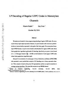
Fig. 4. Asymptotic thresholds and the achievable regions of different codes in binary asymmetric channels.

From TABLE I, we observe that 12A outperforms 12B in Gaussian channels (in which 12A is optimized), but 12B is superior in z-channels for which it is optimized. The above behavior promises room for improvement with codes optimized for different channels, as also shown in [14]. Fig. 4 demonstrates the asymptotic thresholds of these codes in binary asymmetric channels (BASCs) with the curves of 12A and 12B very close together. It is shown that 12B is better when 0 , 1 → 0 or 0 ≈ 1 . We notice that all the achievable regions of these codes are bounded by the symmetric mutual information rate (with (1/2, 1/2) a priori distribution), which is also suggested in [16]. The difference between the symmetric mutual information rate and the capacity for nonDecember 30, 2004

DRAFT

26

DRAFT 0

n= 10 00 0 n= 10 00 0

−2

10

10

(3,6) 12A 12B 12C

00

n=10

00

n=10

−1

*

ε1 of 12A→ ← ε* of 12B 1 *

ε1 of (3,6)→

−6

*

← ε1 of 12C

−4

Symmetric Info Rate→

0.1

0.15

ε

0.2

0.25

10

(a) Bit error rates Fig. 5.

n=1000 0

00 10 n=

−3

10

−5

10

10

n=1000 0

−2

10

000

0

000

000 n=1

n=1000 0

n=1

10 n=

n=1

000

000

10

n=1000 0

−4

0

00

00

n=10

n=1

block error probability

−3

10

n=1

bit error probability

10

0.3

10

(3,6) 12A 12B 12C 0.1

* 1

* 1

ε of 12A→ ← ε of 12B * 1

ε of (3,6)→

* 1

← ε of 12C Symmetric Info Rate→

0.15

ε10

0.2

0.25

(b) Block error rates

Bit/block error rates versus 1 with fixed 0 = 0.00001. Computed thresholds for symmetric

mutual information rate, (3,6), 12A, 12B, and 12C codes are 0.2932, 0.2305, 0.2710, 0.2730, and 0.2356. 40 iterations of belief propagation algorithms were performed. 10,000 codewords were used for the simulations.

symmetric channels is generally indistinguishable from the practical point of view. For example, in [33], it was shown that the ratio between the symmetric mutual information rate and the capacity is lower bounded by

e ln 2 2

≈ 0.942. [34] further proved that the absolute difference is

upper bounded by 0.011 bit/sym. More discussions on capacity achieving codes with non-uniform a priori can be found in [35]. Figs. 5(a) and 5(b) consider several fixed finite codes in z-channels. We arbitrarily select graphs from the code ensemble with codeword lengths n =1,000 and n =10,000. Then, with these graphs (codes) fixed, we find the corresponding parity matrix A, use Gaussian elimination to find the generator matrix G, and transmit different codewords by encoding equiprobably selected information messages. Belief propagation decoding is used with 40 iterations for each codeword. 10,000 codewords are transmitted, and the overall bit/block error rates versus different 1 are plotted for different code ensembles and codeword lengths. Our new density evolution predicts the waterfall region quite accurately when bit error rates are of main interest. Though there are still gaps between the finite codes and our asymptotic thresholds, the performance gaps between different finite length codes are very well predicted by the difference between their asymptotic thresholds. From the above observations and the underpinning theorems, we see that our new density evolution is a successful generalization of the traditional one from both practical and DRAFT

December 30, 2004

0.3


12A, n=1000 12B, n=1000 12A, n=10000 12B, n=10000

ε =0.01 0

ε =0.01 0

ε= 0 0.0 1

ε= 0 0.0 1

ε =0.07 0

7

ε =0 .07 0

ε =0 0 .0

ε =0. 01 0

1

=0 0

10

−4

10

ε =0 .0 0

.0 1 .0 1

=0 ε

0

ε

ε= 0 0.0 7 ε =0 0 .07

−4

−3

10

7


.0 7 =0

7

0

ε

10

ε= 0 0.0


−3

(3,6), n=1000 12C, n=1000 (3,6), n=10000 12C, n=10000

−2

10

ε =0 .0 0

−2

10

27

−5

10 −5

10

* 1

* 1

* 1

ε of 12A→ ← ε of 12B

* 1

* 1

ε of 12B→ ← ε of 12A ← Symmetric Info Rate

* 1

* 1

ε of (3,6)→ ← ε of 12C

ε of (3,6)→

* 1

← ε of 12C

← Symmetric Info Rate



−6

0

0.05

0.1

0.15 ε10

0.2

(a) 12A & 12B:

0.25

0.3

10

0

0.05

0.1

0.15 ε

0.2

0.25

10

(b) 12C & regular (3,6) codes

Fig. 6. Bit error rates versus 1 for 0 = 0.01 and 0 = 0.7. The DE thresholds of (12A, 12B, 12C, (3,6)) are (0.2346, 0.2332, 0.2039, 0.1981) for 0 = 0.01 and (0.1202, 0.1206, 0.1036, 0.0982) for 0 = 0.07. 40 iterations of belief propagation algorithms were performed. 2,000 codewords were used for the simulations.

theoretical points of view. Fig. 5(b) exhibits the block error rate of the same 10,000-codeword simulation. The conjecture of bad block error probabilities for λ2 > 0 codes is confirmed. Besides the conjectured bad block error probabilities, Figs. 5(a) and 5(b) also suggest that codes with λ 2 = 0 will have a better error floor compared to those with λ2 > 0, which can be partly explained by the comparatively slow convergence speed stated in the sufficient stability condition for λ2 > 0 codes. 12C is so far the best code we have for λ2 = 0. However, its threshold is not as good as those of 12A and 12B. If good block error rate and low error floor are our major concerns, 12C (or other codes with λ2 = 0) can still be competitive choices. Recent results in [36] shows that the error floor for codes with λ2 > 0 can be lowered by carefully arranging the degree two variable nodes in the corresponding graph while keeping similar waterfall threshold. Figs. 6(a) and 6(b) illustrate the bit error rates versus different BASC settings with 2,000 transmitted codewords. Our computed density evolution threshold is again highly correlated with the performance of finite length codes for different asymmetric channel settings. We close this section by highlighting two applications of our results. 1. Error Floor Analysis: “The error floor” is a characteristic of iterative decoding algorithms, which is of practical importance and may not be able to be determined solely by simulations. More analytical tools are needed to find error floors for corresponding codes. Our convergence December 30, 2004

DRAFT

0.3

28

DRAFT

- lin. LDPC ENC

-

- lin. LDPC DEC -

Non-sym. CH.

(a) Linear Code Ensemble versus Non-symmetric Channels Symmetric Channel

-

Rand. Bits

- lin. LDPC ENC

h - +?

-

Non-sym. CH.

h - lin. LDPC DEC - +?

(b) Linear Code Ensemble versus Symmetrized Channels LDPC Coset ENC

LDPC Coset DEC

-

Rand. Bits

- lin. LDPC ENC

- +? h

-

Non-sym. CH.

?- +h lin. LDPC DEC -

(c) Coset Code Ensemble versus Non-symmetric Channels Fig. 7. Comparison of the approaches based on codeword averaging and the coset code ensemble.

rate statements in the sufficient stability condition may shed some light on finding codes with low error floors. 2. Capacity-Approaching Codes for General Non-Standard Channels: Various very good codes (capacity-approaching) are known for standard channels, but very good codes for non-standard channels are not yet known. It is well known that one can construct capacity-approaching codes by incorporating symmetric-information-rate-approaching linear codes with the symbol mapper and demapper as an inner code [28], [35], [37]. Understanding density evolution for general memoryless channels allows us to construct such symmetric-information-rate-approaching codes (for non-symmetric memoryless channels), and thus to find capacity-approaching codes after concatenating the inner symbol mapper and demapper. It is worth noting that intersymbol interference channels are dealt with by Kavˇcić et al. in [16] using the coset codes approach. It will be of great help if a unified framework for non-symmetric channels with memory can be found by incorporating both coset codes and codeword averaging approaches.

DRAFT

December 30, 2004


29

Regular (3,4) Code on Z−channel w. pe=(0.00001, 0.4540)

0

10

−1

10

−2

10

p (symmetrized ch) e

CBP (symmetrized Ch) p (x=0)

−3

10

e

p (x=1) e

passing threshold

−4

10

0

100

200 300 Number of Iterations

400

500

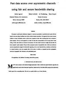
Fig. 8. Density evolution for z-channels with the linear code ensemble and the coset code ensemble.

VII. Side Results of the Generalized Density Evolution

A. Typicality of Linear LDPC Codes

One reason that the non-symmetric channels are overlooked is we can always transform a non-symmetric channel into a symmetric channel. Depending on different points of view, this channel-symmetrizing technique is named the coset code argument [16] or dithering/the i.i.d. channel adapter [21], as illustrated in Figs. 7(b) and 7(c). Our generalized density evolution provides a simple way to directly analyze the the linear LDPC code ensemble on non-symmetric channels, as in Fig. 7(a). It was conjectured in [21] that the scheme in Fig. 7(a) should have the same/similar performance as those illustrated by Figs. 7(b) and 7(c). This short subsection is devoted to this question. In sum, the performance of the linear code ensemble is very unlikely to be identical to that of the coset code ensemble. However, when the minimum d c,min := {k ∈ N : ρk > 0} is relatively large, we can prove that their performance discrepancy is theoretically indistinguishable. In practice, the discrepancy for dc,min ≥ 6 is < 0.05%. (l)

(l)

Let Pa.p. (0) := P (l) (0) and Pa.p. (1) := P (l) (1) ◦ I −1 denote the two evolved densities with (l)

(l)

aligned parity, and similarly define Qa.p. (0) := Q(l) (0) and Qa.p. (1) := Q(l) (1) ◦ I −1 . Our main December 30, 2004

DRAFT

30

DRAFT

TABLE II Threshold comparison p∗1→0 of linear and coset LDPC codes on Z-channels

(λ, ρ)

(x2 , x3 )

(x2 , 0.5x2 + 0.5x3 )

(x2 , x5 )

(x2 , 0.5x4 + 0.5x5 )

Linear

0.4540

0.5888

0.2305

0.2689

Coset

0.4527

0.5908

0.2304

0.2690

result in (15) can be rewritten in the following form: (l) (0) (l−1) Pa.p. (x) = Pa.p. (x) ⊗ λ Qa.p. (x) (l−1)

(l−1) Qa.p. (x) = Γ−1

ρ Γ

(l−1)

Pa.p. (0) + Pa.p. (1) 2 (l−1)

x

+(−1) ρ Γ

!! (l−1)

Pa.p. (0) − Pa.p. (1) 2

!!!

. (0)

It is clear from the above formula that when the concerned channel is symmetric, P a.p. (0) = (0)

Pa.p. (1), it collapses to the traditional density evolution. Since the variable node iteration involves (l−1)

convolution of several densities given the same x value, the difference between Q a.p. (0) and (l−1)

Qa.p. (1) will be amplified after each variable node iteration. Hence it is very unlikely that the decodable thresholds of linear codes and coset codes will be analytically identical. Fig. 8 demonstrates the traces of the evolved densities for the regular (3,4) code on z-channels. With the one-way crossover probability being 0.4540, the generalized density evolution for linear codes is able to converge within 179 iterations, while the channel symmetrizing approach does not show convergence within 500 iterations. This demonstrates the possible performance discrepancy though we do not have analytical results proving that the latter will not converge after more iterations. TABLE II compares the decodable thresholds such that the density evolution enters the stability region within 100 iterations. We notice that the larger d c,min is, the smaller the discrepancy is. This phenomenon can be characterized by the following theorem. Theorem 7: Consider non-symmetric memoryless channels and a fixed pair of degree polynomials λ and ρ. The shifted version of the check node polynomial is denoted as ρ∆ = x∆ · ρ where (l)

∆ ∈ N. Let Pcoset denote the evolved density from the coset code ensemble with degrees (λ, ρ∆ ), P (l) and hP (l) i = 21 x=0,1 Pa.p. (x) denote the averaged density from the linear code ensemble with D

(l)

degrees (λ, ρ∆ ). For any l0 ∈ N, lim∆→∞ hP (l) i = Pcoset in distribution for all l ≤ l0 , with the convergence rate for each iteration being O const∆ for some const < 1.

DRAFT

December 30, 2004


31

Corollary 5: The decodable thresholds of the linear and the coset LDPC codes converge for relatively large ∆. Proof of Theorem 7: The density evolution provides two iterative functionals on the density, and one can easily prove that these functionals are continuous with respect to the convergence in distribution. Therefore, we only need to show that ∀l ∈ N, D

(l−1) (l−1) lim Qa.p. (0) = lim Qa.p. (1)

∆→∞ D

= Γ

−1

∆→∞ (l−1) Pa.p. (0)

ρ Γ

(l−1)

(l−1)

+ Pa.p. (1) 2

!!!

(l−1)

Qa.p. (0) + Qa.p. (1) = , 2

(23)

D

where = denotes the convergence in distribution. Without loss of generality,4 we may assume ρ∆ = x∆ and prove the weak convergence of distributions on the domain m γ(m) := 1{m≤0} , ln coth = (γ1 , γ2 ) ∈ GF(2) × R+ , 2

on which the check node iteration becomes

γout,∆ = γin,1 + γin,2 + · · · + γin,∆ . (l−1)

Let P00 denote the density of γin (m) given the distribution of m being Pa.p. (0) and P10 corre(l−1)

sponds to Pa.p. (1). Similarly let Q00,∆ and Q01,∆ denote the output distributions on γout,∆ when the check node degree is ∆ + 1. It is worth noting that any pair of Q00,∆ and Q01,∆ can be mapped (l−1)

(l−1)

bijectively to the LLR distributions Qa.p. (0) and Qa.p. (1). Let ΦP 0 (k, r) := EP 0 (−1)kγ1 eirγ2 , ∀k ∈ N, r ∈ R, denote the Fourier transform of the density

P 0 . Proving Eq. (23) is equivalent to showing ∀k ∈ N, r ∈ R,

lim ΦQ00,∆ (k, r) = lim ΦQ01,∆ (k, r). ∆→∞

∆→∞

However, to deal with the strictly growing average of the “limit distribution”, we concentrate on the distribution of the normalized output ∀k ∈ N, r ∈ R, 4

γout,∆ ∆

lim ΦQ00,∆ (k,

∆→∞

instead. We then need to prove that r r ) = lim ΦQ01,∆ (k, ). ∆→∞ ∆ ∆

(l−1) ∈ R+ almost surely. This assumption We also need to assume that ∀x, Pa.p. (x)(m = 0) = 0 so that ln coth m 2

can be relaxed by separately considering the event that min,i = 0 for some i ∈ {1, · · · , dc − 1}. December 30, 2004

DRAFT

32

DRAFT

We first note the following iterative equations: ∀∆ ∈ N, r r r r ΦQ00,∆−1 (k, ∆ )ΦP00 (k, ∆ ) + ΦQ01,∆−1 (k, ∆ )ΦP10 (k, ∆ )

r ΦQ00,∆ (k, ) = ∆ r ΦQ01,∆ (k, ) = ∆

2 r r r r )ΦP10 (k, ∆ ) + ΦQ01,∆−1 (k, ∆ )ΦP00 (k, ∆ ) ΦQ00,∆−1 (k, ∆ 2

.

By induction, the difference thus becomes r r r r ΦQ00,∆−1 (k, ) − ΦQ01,∆−1 (k, ) ΦQ00,∆ (k, ) − ΦQ01,∆ (k, ) = ∆ ∆ ∆ ∆ ! ∆ r r ΦP00 (k, ∆ ) − ΦP10 (k, ∆ ) = 2 . 2

r r ) − ΦP10 (k, ∆ ) ΦP00 (k, ∆

2

!

(24)

By Taylor expansion and the BASC decomposition argument in [29], we can show that for all k ∈ N, r ∈ R, and for all possible P00 and P10 , (24) converges to zero with convergence rate O const∆ for some const < 1. Detailed derivation of the convergence rate is in Appendix III.

Since the limit of the right-hand side of (24) is zero and the proof of weak convergence is complete. The exponentially fast convergence rate O const∆ also justifies the fact that even for small

dc,min ≥ 6, the performances of linear and coset LDPC codes are very close.

(l−1)

Remark 1: Consider any non-perfect message distribution, namely, ∃x0 such that Pa.p. (x0 ) 6= D

(l−1)

δ∞ . A persistent reader may notice that ∀x, lim∆→∞ Qa.p. (x) = δ0 , namely, as ∆ becomes large, all information is erased after passing a check node of large degree. If this convergence (erasure (l−1)

(l−1)

effect) occurs earlier than the convergence of Qa.p. (0) and Qa.p. (1), the performances of linear and coset LDPC codes are “close” only when the code is “useless.”5 To quantify the convergence rate, we consider again the distributions on γ and their Fourier transforms. For the average of (l−1)

the output distributions Qa.p. (x), we have r r ΦQ00,∆ (k, ∆ ) + ΦQ01,∆ (k, ∆ )

2

=

=

r r ) + ΦQ01,∆−1 (k, ∆ ) ΦQ00,∆−1 (k, ∆

2 r r ΦP00 (k, ∆ ) + ΦP10 (k, ∆ )

2

!∆

.

!

r r ΦP00 (k, ∆ ) + ΦP10 (k, ∆ )

2

!

(25)

By Taylor expansion and the BASC decomposition argument, one can show that the limit of (25) exists and the convergence rate is O(∆−1 ). (Detailed derivation is in Appendix III.) This convergence rate is much slower than the exponential rate O const∆ in the proof of Theorem 7. 5

To be more precise, it corresponds to an extremely high-rate code and the information is erased after every

check node iteration. DRAFT

December 30, 2004

WANG, KULKARNI, POOR: DENSITY EVOLUTION ON SYMBOL-DEPENDENT CHANNELS The check node iteration, w. dc=6, one−way p1→ 0:0.2305

1

x=0 x=1 average

0.9 0.8 0.7 0.6 0.5 0.4 0.3 0.2 0.1 0 −2.5

The check node iteration, w. dc=10, one−way p1→ 0:0.2305 x=0 x=1 average

0.9 Cumulative Distribution Function

Cumulative Distribution Function

1

33

0.8 0.7 0.6 0.5 0.4 0.3 0.2 0.1

−2

−1.5

−1

−0.5

0 mout

0.5

1

1.5

2

0 −2.5

2.5

(l−1)

−2

−1.5

−1

−0.5

0 mout

0.5

1

(l−1)

1.5

2

2.5

(l−1)

Fig. 9. The weak convergence of Qa.p. (0) and Qa.p. (1). One could tell that the convergence of Qa.p. (0) (l−1)

and Qa.p. (1) is faster than the convergence of

(l−1) Q(l−1) a.p. (0)+Qa.p. (1) 2

and δ0 .

Therefore, we do not need to worry about the case that the required ∆ for the convergence of (l−1)

(l−1)

(l−1)

D

Qa.p. (0) and Qa.p. (1) is excessively large such that ∀x ∈ GF(2), Qa.p. (x) ≈ δ0 . Remark 2: The intuition behind Theorem 7 is when the minimum dc is sufficiently large, the parity check constraint becomes relatively less stringent. Thus we can approximate the density of the outgoing messages for linear codes by assuming all bits involved in that particular parity check equation are “independently” distributed among {0, 1}, which becomes exactly the formula for the coset code ensemble. However, extremely large dc is required for a check node iteration to completely destroy all information coming from the previous iteration. This explains the difference of their convergence rates O const∆ and O(∆−1 ). Fig. 9 demonstrates the weak convergence in Theorem 7 and visualizes the convergence rates (l−1)

(l−1)

of Qa.p. (0) −→ Qa.p. (1) and

(l−1)

(l−1)

Qa.p. (0)+Qa.p. (1) 2

→ δ0 .

B. Revisit the Belief Propagation Decoder There are two known facts about the BP algorithm and the density evolution method. First, the BP algorithm is optimal for any cycle-free network, since it exploits the independence of the incoming LLR message. Second, by the cycle-free convergence theorem, the traditional density evolution is able to predict the behavior of the BP algorithm (designed for the tree structure) for l0 iterations, even when we are considering the Tanner graph of a LDPC code with finite but sufficiently large codeword length n. The performance of BP, predicted by the density evolution, is outstanding so that we “implicitly assume” that the BP (designed for the tree structure) is December 30, 2004

DRAFT

34

DRAFT

also optimal for the first l0 iterations in terms of minimizing the codeword-averaged bit error rate (ber). To be able to consider the codeword-averaged ber, the optimal decision inevitably has to exploit the global knowledge about all possible codewords, which is, however, not available to the BP decoder. The question needs to be answered is whether BP is still optimal when the global information about the entire codebook is accessible and the computational power is unlimited? The answer is a straightforward corollary of Theorem 3, the convergence to perfect projection, which provides the missing link regarding to the optimality of BP when only local observations are available. Theorem 8 (The Optimality of the BP Decoder) For sufficiently large codeword length n, alˆ BP (Yl0 ) most all instances in the random code ensemble have the property that the BP decoder X ˆ M AP,l (Y l0 ), where l0 is a fixed after l0 iterations coincides with the optimal MAP bit detector X 0 ˆ M AP,l (·) uses the same amount of observations as in X ˆ BP (·) integer. The MAP bit detector X 0 but is able to exploit the global knowledge about the entire codebook. Proof:

2l0 When the support tree N(i,j) is perfectly projected, the local information about

the tree-satisfying strings is equivalent to the global information about the entire codebook. By Theorem 3, we thus show that for sufficiently large n, the extra information about the codebook does not benefit the decision maker, and the BP decoder is optimal. Note: Even for symmetric memoryless channels, the optimality of BP in terms of global codebook knowledge can only be proved by the convergence to perfect projection. Theorem 8 can thus be viewed as a completion of the classical density evolution for symmetric memoryless channels. VIII. Conclusions In this paper, we have developed a codeword-averaged density evolution, which allows analysis of general non-symmetric memoryless channels. An essential perfect projection convergence theorem has been provided using the analysis of constraint propagation and the behavior of random matrices. With the perfect projection convergence theorem, the theoretical foundation of the codeword-averaged density evolution is well established. Most of the properties of symmetric density evolution have been restated and proven for the codeword-averaged density evolution on non-symmetric channels, including monotonicity, distribution symmetry, and stability. Besides a necessary stability condition, a sufficient stability condition has been stated with convergence rate arguments and a simple proof. DRAFT

December 30, 2004


35

The typicality of the linear LDPC code ensemble has been proved by the weak convergence (w.r.t. dc ) of the evolved densities in our codeword-averaged density evolution. Namely, when the check node degree is sufficiently large (e.g. dc ≥ 6), the performance of linear LDPC code ensemble is very close to (e.g. within 0.05%) the performance of the LDPC coset code ensemble. One important corollary of the perfect projection convergence theorem is the optimality of the belief propagation algorithms when the global information about the entire codebook is accessible. This can be viewed as a completion of the classical density evolution where symmetric memoryless channels are of major interest. Extensive simulations have been presented, the degree distribution has been optimized for zchannels, and possible applications of our results have been discussed as well. From both practical and theoretical points of view, our codeword-averaged density evolution offers a straightforward and successful generalization of the traditional symmetric density evolution for general nonsymmetric memoryless channels. Appendices I. Proof of Theorem 3 We first introduce the following corollary of Theorem 1. Corollary 6 (Cycle-free Convergence) For a sequence ln such that ((dv − 1)(dc − 1))2ln = o(n), we have for any i0 , j0 , lim P N(i2l0n,j0 ) is cycle-free = 1.

n→∞

Proof of Theorem 3: We first show that for any fixed l, lim P N(i2l0 ,j0 ) is perfectly projected = 1,

n→∞

and discuss the convergence rate later. We notice that if for any ln ≥ l, N(i2l0n,j0 ) is perfectly projected, then so is N(i2l0 ,j0 ) . Choose ln =

ln n 4 9 ln(dv −1)+ln(dc −1) .

By Corollary 6, we have

lim inf P(N(i2l0 ,j0 ) is perfectly projected) n→∞ 2(ln +1) 2(ln +1) 2ln ≥ lim inf P N(i0 ,j0 ) is perfectly projected N(i0 ,j0 ) is cycle-free P N(i0 ,j0 ) is cycle-free n→∞

2(l +1)

+ lim P(N(i0 ,jn0 ) is not cycle-free) n→∞ 2(l +1) = lim inf P N(i2l0n,j0 ) is perfectly projected N(i0 ,jn0 ) is cycle-free .

(26)

n→∞

December 30, 2004

DRAFT

36

DRAFT

We then need only to show that 2(l +1)

lim P(N(i2l0n,j0 ) is perfectly projected|N(i0 ,jn0 )

n→∞

is cycle-free) = 1.

(27)

To prove (27), we take a deeper look at the incidence matrix (the parity check matrix) A. We take the (3, 5) regular code as our illustrative example. Suppose the codeword length n is large enough so that ln ≥ l. Conditioning on the event that the graph is cycle-free until depth 2 ∗ 2, we can transform A into the following form by row and column swaps, with ⊗ also used as the Kronecker product (whether it represents convolution or Kronecker product should be clear in the context). 



1 1 1 1 1

1 1       A =        

1 1 1 1 1 1 1 1

1

1 1 1 1

1

1 1 1 1 1

1 1 1 1

1

1 1 1 1 1

1 1 1 1

1

1 1 1 1 1

1 1 1 1

1

1 1 1 1 ···

1



0 0  I1×1 ⊗ (1, 1, 1, 1, 1)   I5×5 ⊗ 11 I10×10 ⊗ (1, 1, 1, 1) 0  =   0 I40×40 ⊗ 11 A080×(n−45)   0 0 A00( 3n −91)×(n−45) 5



where Ia×a denotes the a × a identity matrix, 

A080×(n−45)

A00( 3n −91)×(n−45) 5



               

    ,   



 is the incidence matrix of

the equiprobable, bipartite subgraph, in which (n − 45) variable nodes have degree d v , 80 check nodes have degree dc − 1, and ( 3n 5 − 91) check nodes have degree dc . Conditioning on a more

2 ∗ 2, we will have  0   0  ,  0 A   00 A is composed of one I1×1 ⊗ (1, 1, 1, 1, 1) and (ln − 1) pairs of I ⊗ 11 and I ⊗ (1, 1, 1, 1).

general event that the graph is cycle free until depth 2(ln + 1) rather than  A ln 0    0 I(5∗8ln −1 )×(5∗8ln −1 ) ⊗ 11 I(10∗8ln −1 )×(10∗8ln −1 ) (1, 1, 1) A=   0 I(5∗8ln )×(5∗8ln ) ⊗ 11  0 0

where Aln A0 0 00 A00 is the incidence matrix with rows (check nodes) in A and A having degree (dc − 1) and DRAFT

December 30, 2004


37

dc . For convenience, we denote the blocks in A as 

A ln

0

   0 Tln A=   0  0

Uln +1 Tln +1 0

0



  0  .  A0   A00

Then N(i2l0n,j0 ) is not perfectly projected if and only if there exists a non-zero row vector (r|0|0) such that 

  (r|0|0) ∈ RowSpace  

0 Tln

Uln +1

0

0

Tln +1

A0

0

0

A00



  , 

(28)

and r is not in the row space of Aln , or equivalently (r|0|0) is not in RowSpace(Aln |0|0).

(29)

Eqs. (29) and (28) say that there exists a constraint r on these N(i2l0n,j0 ) variable nodes, which is V not from the linear combination of those N(i2l0n,j0 ) check node equations, but rather is imposed C

by the parity check equations outside N(i2l0n,j0 ) .

From (28), we know that, for (r|0|0) to exist, there must exist a non-zero row vector (0|s|0) such that 

(0|s|0) ∈ RowSpace 

0 Tln +1

A0

0

A00

0



,

(30)

and s ∈ RowSpace(Uln +1 ) = RowSpace I(10∗8ln −1 )×(10∗8ln −1 ) ⊗ (1, 1, 1, 1) .

(31)

From (31), the 1’s in s must be aligned such that four neighboring bits should have the same value; for example, s = (111100001111000000001111 · · · 00001111). Any non-zero s satisfying (30) is generated by Tln +1 . By applying the row symmetry in A0 , we see that the 1’s in any s are uniformly distributed among all these 5 ∗ 8ln bits. So for an s December 30, 2004

DRAFT

38

DRAFT

that is not all-one, the probability that the 1’s in that s are aligned is P s ∈ RowSpace I(10∗8ln −1 )×(10∗8ln −1 ) ⊗ (1, 1, 1, 1)

≤ P(the 1’s in s are aligned) ln −1 −1 10∗8X 10∗8ln −1 a = · P(there are 4a ones in s) 5∗8ln a=1

≤

10∗8ln −1 1 5∗8ln 4

4a

1 = O( ((dv − 1)(dc − 1))ln

dc −2

4

) = O(n− 9 (dc −2) ).

(32)

The last inequality follows from the assumption that s is neither all-zero nor all-one. The reason why we can exclude the case that s is all-one is that, if dv is odd, then there is an even number of 1’s in each column of Tln . Since there is only one 1 in each column of Uln +1 , by (28), an all-one s can only generate an all-zero r, which puts no constraints on N (i2l0n,j0 ) . If dv is even, by 5·8ln −1

z }| { the same reasoning, an all-one s will generate r of the form (00 · · · 0 11 · · · 1). Nevertheless, when

dv is even, this specific type of r is in the row space of Aln , which does not fulfill the requirement

in (29). From the above reasoning, we can exclude the all-one s. A0 A0 The number of vectors s minus Rank( A Let mr denote the number of rows of A 00 ). 00 satisfying (30) is bounded by 2mr . By Proposition 4 (which will be formally stated and proved

later), we have P(2mr ≥ n1.1 ) = O(n−0.1 ). We note that conditioned on the rank of

A0 A00

(33)

, the 1’s in s are uniformly distributed and (32)

still holds. Therefore by (32) and (33), we have

2(l +1)

lim sup P(N(i2l0n,j0 ) is not perfectly projected|N(i0 ,jn0 ) n→∞

is cycle-free)

≤ lim sup P(∃r satisfying (28) and (29)) n→∞

≤ lim sup P(∃s, which satisfies (30) and (31), but is not all-one) n→∞ 4 ≤ lim sup n1.1 O(n− 9 (dc −2) )P(2mr ≤ n1.1 ) + P(2mr > n1.1 ) = 0, n→∞

(34)

where the last inequality follows from the simple union bound with respect to the total number of possible s. Eq. (34) holds when dc ≥ 5, i.e. we have proved Theorem 3 for dc ≥ 5 (without the convergence rate argument). To prove the case dc < 5, we focus on the probability that the constraints propagate two levels rather than just one level, i.e. instead of (27), we focus on DRAFT

December 30, 2004


39

proving the following limit. 2(l +2)

lim P(N(i2l0n,j0 ) is perfectly projected|N(i0 ,jn0 )

ln →∞

is cycle-free) = 1.

Most of the analysis remains the same. Eq. (32) will be replaced by P((0|s|0) is able to propagate two levels) = P((0|s|0) propagates the 2nd level|(0|s|0) propagates the 1st level) · P((0|s|0) is propagate the 1st level)

10∗8ln 10∗8ln −1 a ≤ 5∗8ln 5∗8lbn +1 4b 4a ln −1 10∗8ln 1 (a) 10∗8 1 4 ≤ 5∗8ln +1 5∗8ln 4∗4 4

1 = O( ((dv − 1)(dc − 1))ln

dc −2

1 ((dv − 1)(dc − 1))ln

(dc −1)(dc −2)

4

2

) = O(n− 9 (dc −2dc ) ),

where a and b are the numbers of rows involved in Uln +1 and Uln +2 , and the inequality marked (a) follows by studying the necessary number of rows to propagate levels (l n + 1) and (ln + 2). With this stronger inequality, we thus complete the proof of the case dc ≥ 3 for all regular codes of practical interest. Convergence Rate: We take a closer look at the derived inequalities. By (33), (34) is bounded by O(n−0.1 ). Then by Theorem 1, the convergence rate of (26) is bounded by O(n−0.1 ) +

O(n−1/9 )) = O(n−0.1 ), which completes the analysis. Note that this convergence rate upper bound is not tight and can be improved by following the same steps but considering the propagation of three levels instead of two, which however is not our main purpose.

We close this section by stating the proposition regarding mr , the number of linearly dependent A0 rows in A 00 . The proof is left to Appendix II. n Proposition 4: Consider the code ensemble Cm 0 ,m00 (dv , dc ) generated by equiprobable edge per-

mutation on a bipartite graph with n variable nodes of degree dv , m0 and m00 check nodes with A0 degree (dc − 1) and dc , and m0 = o(n). The corresponding parity check matrix is A = A 00 .

With mr denoting the number of linearly dependent rows in A, i.e. mr := m0 + m00 − Rank(A), we have

which automatically implies P 2mr December 30, 2004

E{2mr } = O(n), > n1+α = P mr >

(1+α) ln n ln 2

= O(n−α ), for any α > 0. DRAFT

40

DRAFT

Corollary 7: Let R denote the rate of a regular LDPC code ensemble C n (dv , dc ), i.e., R =

n−Rank(A) , n

in L1 , i.e.

Proof:

where A is the corresponding parity check matrix. Then R converges to (n − m)/n n − m lim E R − = 0. n→∞ m It is obvious that R ≥ n−m n . To show that lim supn→∞ E{R −

m1 = 0, rewrite R =

n−Rank(A) n

=

n−m n

+

mr n .

n−m n }

= 0, we let

By Proposition 4 and the fact that

≤ 1, we

have limn→∞ E{ mnr } = 0. The proof is complete.

mr n

A stronger version of the convergence of R with respect to the block length n can be found in [30]. II. Proof of Proposition 4 We finish the proof of Proposition 4 by first stating the following lemma, inequality and theorem. Lemma 2 (Lemma 3.2 in [38]) For any m × n matrix A over GF(2) with m ≤ n and m r = m − Rank(A), we have 2 mr =

|CA | + 1 , 2n−m

where CA is the collection of all non-empty subsets of column vectors such that for each subset, the GF(2) sum of its elements is 0. Inequality 1: Using Stirling’s double inequality, √ √ 1 1 1 1 2πn(n+ 2 ) e(−n+ 12n+1 ) < n! < 2πn(n+ 2 ) e(−n+ 12n ) , we have s 1 1 1 nH2 (θ) 1 − 1 − √ 2 e 12n+1 12θn 12(n−θn) nθ(1 − θ) 2π s 1 1 n 1 nH2 (θ) 1 − 1 − e 12n 12θn+1 12(n−θn)+1 , < 0.

Then, for δ > 0,   P P Pm n m j=1 kj (kj − 1) ( i=1 li (li − 1))  j=1 kj ! − k,l Q −1+δ Q . 1 + o n = exp Λ m,n   P 2 n m m i=1 li ! j=1 kj ! 2 j=1 kj

We note that the above theorem is focused on integer matrices, rather than those with elements

in GF(2). By the same technique used in [24], we let A be the expanded, non-negative integer matrix of the parity check matrix A, where A is an m × ndv matrix such that kj = dc − 1 for j ∈ [1, m0 ], kj = dc for j ∈ [m0 + 1, m], and li = 1 for i ∈ [1, ndv ]. We note that A can be n mapped to graphs in Cm 0 ,m00 (dv , dc ), with columns ((i − 1)dv + 1) to idv corresponding to all

edges of variable node i. Therefore, it is equivalent to consider the equiprobable matrix ensemble dc ,1 Λm 0 ,m00 ,nd containing all these A’s. v dc ,1 dc ,1 Let Λnd denote the subset of Λm 0 ,m00 ,nd such that the GF(2) sum of columns 1 to (bθncd v ) v ,θ v

equals 0. Then dc ,1 Λndv ,θ

. P (the set of “columns 1 to bθnc” is in CA ) = d ,1 Λmc0 ,m00 ,ndv

By Lemma 2 and the symmetry between different variable nodes, the statement in Proposition 4 is equivalent to E |CA | 1 = n−m n−m n2 n2

Λdc ,1 Z 1 n Λdc ,1 n X ndv ,θ ndv ,θ n bθnc = dθ = O(1), n−m d ,1 d ,1 c bθnc Λ c0 00 0 2 Λ 0 00 θn=1 m ,m ,ndv m ,m ,ndv

(36)

where O(1) is a positive constant independent of n and θ. Proof of Proposition 4:

Letting m00 , m02 , . . . , m0

2b d2c c

denote the number of rows in rows

1 ∼ m0 with sums of columns 1 ∼ dv bθnc equal to 0, 2, · · · , 2b d2c c, and let m000 , m002 , . . . , m00

2b d2c c

December 30, 2004

DRAFT

42

DRAFT

denote the corresponding quantities in rows (m0 + 1) ∼ m. Then we have m00 + m02 + · · · + m02b dc c = m0

(37)

m000 + m002 + · · · , m002b dc c = m00

(38)

2

2

2(m02 + m002 ) + 4(m04 + m004 ) + · · · + 2b

dc c(m02b dc c + m002b dc c ) = bθncdv , 2 2 2

(39)

and

where “

dc ,1 Λndv ,θ =

P

(37),(38),(39) ”

X

(37),(38),(39)

m0 m00 , · · · , m0

2b d2c c

m00 m000 , · · · , m00

2b d2c c

dc ,1 dc ,1 Lndv ,θ Rndv ,θ ,

means the sum is taken over all possible m00 , · · · , m0

2b d2c c

(40)

and m000 , · · · , m00

2b d2c c

satisfying (37), (38), and (39);

P

ai a1 , · · · , ah

P ai )! := Q ai ! (

is the multinomial coefficient; Ldndc ,1v ,θ is the collection of m×dv bθnc matrices with a fixed row sum distribution kL compatible with m00 , · · · , m0

2b d2c c

and m000 , · · · , m00

2b d2c c

dc ,1 is the collection ; and Rnd v ,θ

of m × (ndv − dv bθnc) matrices with a fixed row sum distribution kR such that kL + kR = k (k is the row sum distribution of A). Essentially, we count the possible configurations by splitting dc ,1 dc ,1 the matrix into its left half Lnd and right half Rnd . v ,θ v ,θ

By Theorem 9 and (39), we have dc ,1 1 + o n−1+δ Lndv ,θ =

(dv bθnc)!

m0 dc +m00 dc 0 00 0 00 (2!)m2 +m2 (4!)m4 +m4 · · · 2b d2c c ! 2b 2 c 2b 2 c (ndv − dv bθnc)! dc ,1 1 + o n−1+δ Rndv ,θ = m0 d c 0 ((dc − 1 − 2)!)m2 · · · dc − 1 − 2b d2c c ! 2b 2 c 1 · m00 dc 00 ((dc − 2)!)m2 · · · dc − 2b d2c c ! 2b 2 c (ndv )! dc ,1 1 + o n−1+δ . Λm1 ,m,ndv = ((dc − 1)!)m0 ((dc )!)m00

(41)

(42) (43)

By (40), (41), (42), and (43), we have dc ,1 n n Λndv ,θ X m0 m00 bθnc bθnc −(n−m) = O(1)2 ndv m00 , · · · , m0 dc m000 , · · · , m00 dc 2n−m Λdc0,1 00 d bθnc 2b 2 c 2b 2 c (37),(38),(39) v m ,m ,ndv m02 m002 m0 m00 dc − 1 2b d2c c dc − 1 dc dc 2b d2c c ··· · (44) dc dc 2b 2 c 2 2b 2 c 2 DRAFT

December 30, 2004


43

We now show that the point-wise limit of (44) is bounded by O(1), then by dominated convergence, we obtain (36). Case 1: θ = 21 . Continuing the analysis of Eq. (44),

n bθnc 2n−m

dc ,1 Λndv ,θ

=

dc ,1 Λm0 ,m00 ,ndv

O(1)2

X

−(n−m) −(dv −1)n

2

(37),(38),(39)

m0 m00 , · · · , m0

2b d2c c

m00 m000 , · · · , m00

2b d2c c

m02 m002 0 m00 dc − 1 m2b d2c c dc dc 2b d2c c ··· dc dc 2b 2 c 2 2b 2 c X m00 m0 O(1)2−(n−m) 2−(dv −1)n 00 0 0 m0 , · · · , m00 m 0 , · · · , m dc

dc − 1 · 2

(a)

≤

=

2b d2c c

c

dc − 1 2

j=0

=

2

m02 m002 0 m00 dc dc − 1 m2b d2c c dc 2b d2c c ··· dc dc 2 2b 2 c 2b 2 c  m00 m0  j≤b d2c c j≤b d2c c dc   X dc − 1   X O(1)2−m−dv n     2j 2j ·

(b)

2b

(37),(38)

O(1)2−m−dv n 2

m0 (d

c −2)

j=0

2

m00 (d

c −1)

= O(1),

(45)

where (a) follows from dropping constraint (39) and (b) follows from the multinomial expansion formula. Case 2: θ 6= 21 . In this case, Eq. (44) can be further analyzed as follows

n bθnc 2n−m (a)

≤

O(1)2

dc ,1 Λndv ,θ

dc ,1 Λm0 ,m00 ,ndv

−(n−m) −(dv −1)nH2 (θ)

2

dc − 1 · 2 (b)

≤

O(1)2

0

00 b d2c c+1

(m m )

max

(37),(38),(39)

m0 m00 , · · · , m0

m02 m002 0 m00 dc − 1 m2b d2c c dc dc 2b d2c c ··· dc dc 2b 2 c 2 2b 2 c

−(n−m) −(dv −1)nH2 (θ)

2

0

00 b d2c c+1+ 12

(m m )

max

(37),(38),(39)

2b d2c c

0

m0m m00m Qb d2c c i=0

m00 m000 , · · · , m00

dc − 1 · 2

December 30, 2004

(37),(38),(39)

2b d2c c

00

0

00

m02i m2i m002i m2i

m02 m002 0 m00 dc dc dc − 1 m2b d2c c 2b d2c c ··· dc dc 2 2b 2 c 2b 2 c dc 1 , max f (θ, m02i , m002i ) O(1)2−(n−m) (m0 m00 )b 2 c+1+ 2 exp n

=

(46) DRAFT

44

DRAFT

where (a) is obtained by (35) and using the maximum times the number of elements to bound the total sum inequality. (b) follows from Stirling’s formula. And f (θ, m02i , m002i )

m0 ln m0

+

m00 ln m00

:= −(dv − 1)H(θ) +

−

Pb d2c c i=0

m02i ln

m02i

(dc2i−1)

+

m00 m002i ln dc2i ( ) 2i

n

.

n Note: w(θ) := limn→∞ max f (θ, (m02i ) , (m002i )) is the asymptotic distance distribution of Cm 0 ,m00 (dv , dc ).

During the derivation of (45), we have shown that w( 21 ) ≤ limn→∞

(n−m) ln 2 n

(dc −dv ) ln 2 . dc

=

If for any θ 6= 1/2, w(θ) < w(1/2), then (46) → 0 as n → ∞, which completes our proof. (∀θ 6= 1/2, w(θ) < w(1/2) agrees with the intuition that most of the codewords in a uniformly randomized code are composed of half zeros and half ones.) w(θ) can be further bounded by the relaxation from integers (m02i ) and (m002i ) to non-negative reals. Using Lagrange multipliers, the optimization problem with constraints (37),(38),(39) has a unique solution as follows. tn is the positive root of tn (1 + tn )dc −1 − (1 − tn )dc −1 bθncdv − O(m0 ) = . (1 + tn )dc + (1 − tn )dc m00 dc 

w(θ) = −(dv − 1)H(θ) + lim  n→∞

= −(dv − 1)H(θ) +

m00 n

dv (1 + ln dc

ln

(1 + tn

) dc

+ (1 − tn

bθncdv −O(m0 ) dc m00 dc

) dc

+

O(m0 )

2tn + (1 − t)dc , 2tdc θ

t)dc

n

 

where t is the only positive root of t (1 + t)dc −1 − (1 − t)dc −1 = θ. (1 + t)dc + (1 − t)dc Notes: (1) t and θ are one-to-one.6 (2) This formula coincides with the asymptotic distance distribution of the regular code ensemble C ∞ (dv , dc ) in [24], which means the small portion of rows (o(n) rows) with degree dc − 1 does not play an important role in the asymptotic distance distribution. To show that θ = 1/2 is the unique maximum point of w(θ), we use two properties from [24], which can also be easily derived using simple calculus. (i) When dc is odd, 6

dw(θ) dθ

< 0 for all

Actually, when dc is even, t ∈ [0, ∞] and θ ∈ [0, 1] are one-to-one and onto. For odd dc , θ must be in [0,

dc −1 ]. dc

Otherwise t will not exist. DRAFT

December 30, 2004


45

θ > 1/2, and (ii) when dc is even, w(θ) is symmetric with respect to θ = 1/2. From (i) and (ii), we need only to consider whether θ = 1/2 is the unique maximum in the range [0, 1/2] (or equivalently t ∈ [0, 1]). From the first and second derivatives of w(θ), it is apparent that θ = 1/2 (or t = 1) is a local maximum. The second derivative of w(θ) is 2 (1 + t)dc + (1 − t)dc w2 (θ) d2 w(θ) = , dθ2 t ((1 + t)2dc −2 − (1 − t)2dc −2 ) ((1 + t)2dc −2 − (1 − t)2dc −2 + 4(dc − 1)t(1 − t2 )dc −2 ) where w2 (θ) = − (1 + t)2dc −2 − (1 − t)2dc −2 + 4(dv − 1)(dc − 1)t(1 − t2 )dc −2 , d2 w(θ) . We note that w2 (0) = 0 and taking the second dθ 2 2 2 (θ) shows d w < 0. Thus the sign of w2 (θ) as θ ranges from dt2

determines the sign of

derivative of w2 (θ)

with respect to t

0 to 1/2 can either

be all negative, or go from positive to negative just once (depending on d v < 2 or dv > 2). In both cases, θ = 1/2 is the unique global maximum of w(θ). From the analysis of whether θ = 1/2, we conclude that the point-wise limit of the integrand in (44) is bounded by O(1). By the dominated convergence theorem, the integral is bounded by O(1), too. We thus obtain (36) and the proof is complete. III. The Convergence Rates of (24) and (25) For (24), we will consider the cases that k = 0 and k = 1 separately. By the BASC decomposition argument, namely, all non-symmetric channels can be decomposed as the probabilistic combination of many BASCs, we can limit our attention to simple BASCs rather than general (l−1)

(l−1)

memoryless non-symmetric channels. Suppose Pa.p. (0) and Pa.p. (1) correspond to a BASC with crossover probabilities 0 and 1 . Without loss of generality, we may assume 0 + 1 < 1 (l−1)

because of the previous assumption that ∀x ∈ GF(2), Pa.p. (x)(m = 0) = 0. We then have 1−0 +1 1+0 −1 r i r ln i r ln ) = (1 − 0 )e ∆ 1−0 −1 + (−1)k 0 e ∆ 1−0 −1 ∆ 1+0 −1 1−0 +1 r i r ln i r ln ΦP10 (k, ) = (1 − 1 )e ∆ 1−0 −1 + (−1)k 1 e ∆ 1−0 −1 . ∆

ΦP00 (k,

By Taylor expansion, for k = 0, (24) becomes !∆ r r ) − ΦP10 (0, ∆ ) ΦP00 (0, ∆ 2 2 ∆ 1 − 0 − 1 r 1 − 0 + 1 r 2 = 2 i , ln +O 2 ∆ 1 + 0 − 1 ∆ December 30, 2004

DRAFT

46

DRAFT

which converges to zero with convergence rate O O(∆)−∆ . For k = 1, we have r r ΦP00 (1, ∆ ) − ΦP10 (1, ∆ )

2

2

!∆

∆ ir r 2 1 + 0 − 1 1 − 0 + 1 = 2 (1 − 0 ) + , − (1 + 0 − 1 ) ln (1 − 0 + 1 ) ln +O 2 ∆ 1 − 0 − 1 1 − 0 − 1 ∆ which converges to zero with convergence rate O(const∆ ), where const satisfies |1 −0 | < const < 1. Since the convergence rate is determined by the slower of the above two. We prove that (24) converges to zero with rate O(const∆ ) for some const < 1. Consider (25). Since we assume that the input is not perfect, we have max( 0 , 1 ) > 0. For k = 0, by Taylor expansion, we have r r ΦP00 (0, ∆ ) + ΦP10 (0, ∆ )

!∆

2 ∆ 1 − 0 + 1 r 2 1 + 0 − 1 ir (1 − 0 + 1 ) ln +O , + (1 + 0 − 1 ) ln = 1+ 2 ∆ 1 − 0 − 1 1 − 0 − 1 ∆ which converges to e

i( 2r ) (1−0 +1 ) ln

1−0 +1 1+ − +(1+0 −1 ) ln 1−0 −1 1−0 −1 0 1

with rate O ∆−1 . For k = 1, we have

r r ΦP00 (1, ∆ ) + ΦP10 (1, ∆ )

2 

= (1 − 0 − 1 )



e

!∆

r ln i∆

1−0 +1 1−0 −1

+e 2

r ln i∆

1+0 −1 1−0 −1

∆

 ,

which converges to zero with rate O (1 − 0 − 1 )∆ . Since the overall convergence rate is the slower of the above two, we prove that the convergence rate is O ∆−1 . References

[1]

C. Berrou and A. Glavieux, “Near optimum error correcting coding and decoding: Turbo-codes,” IEEE Trans. Inform. Theory, vol. 44, no. 10, pp. 1261–1271, Oct. 1996.

[2]

R. G. Gallager, Low-Density Parity-Check Codes, Number 21 in Research Monograph Series. MIT Press, Cambridge, MA, 1963.

[3]

D. J. C. MacKay, “Good error-correcting codes based on very sparse matrices,” IEEE Trans. Inform. Theory, vol. 45, no. 2, pp. 399–431, Mar. 1999.

DRAFT

December 30, 2004


[4]

47

M. Sipser and D. A. Spielman, “Expander codes,” IEEE Trans. Inform. Theory, vol. 42, no. 6, pp. 1710–1722, Nov. 1996.

[5]

J. Pearl, Probabilistic Reasoning in Intelligent Systems: Network of Plausible Inference, Morgan Kaufmann, San Mateo, 1988.

[6]

R. J. McEliece, D. J. C. Mackay, and J. F. Cheng, “Turbo decoding as an instance of Pearl’s “Belief Propagation” algorithm,” IEEE J. Select. Areas Commun., vol. 16, no. 2, pp. 140–152, Feb. 1998.

[7]

S. Y. Chung, G. D. Forney, Jr., T. J. Richardson, and R. L. Urbanke, “On the design of low-density paritycheck codes within 0.0045 dB of the Shannon limit,” IEEE Commun. Letters, vol. 5, no. 2, pp. 58–60, Feb. 2001.

[8]

T. J. Richardson and R. L. Urbanke, “Efficient encoding of low-density parity-check codes,” IEEE Trans. Inform. Theory, vol. 47, no. 2, pp. 638–656, Feb. 2001.

[9]

D. A. Spielman, “Linear-time encodable and decodable error-correcting codes,” IEEE Trans. Inform. Theory, vol. 42, no. 6, pp. 1723–1731, Nov. 1996.

[10] J. W. Byers, M. Luby, and M. Mitzenmacher, “A digital fountain approach to asynchronous reliable multicast,” IEEE J. Select. Areas Commun., vol. 20, no. 8, pp. 1528–1540, Oct. 2002. [11] M. G. Luby, M. Mitzenmacher, M. A. Shokrollahi, and D. A. Spielman, “Analysis of low-density codes and improved designs using irregular graphs,” in Proc. 30th Annu. ACM Symp. Theory of Computing, 1998, pp. 249–258. [12] M. G. Luby, M. Mitzenmacher, M. A. Shokrollahi, and D. A. Spielman, “Efficient erasure correcting codes,” IEEE Trans. Inform. Theory, vol. 47, pp. 569–584, Feb. 2001. [13] T. J. Richardson and R. L. Urbanke, “The capacity of low-density parity-check codes,” IEEE Trans. Inform. Theory, vol. 47, no. 2, pp. 599–618, Feb. 2001. [14] J. Hou, P. H. Siegel, and L. B. Milstein, “Performance analysis and code optimization of low density paritycheck codes on Rayleigh fading channels,” IEEE J. Select. Areas Commun., vol. 19, no. 5, pp. 924–934, May 2001. [15] J. Garcia-Frias, “Decoding of low-density parity check codes over finite-state binary Markov channels,” in Proc. IEEE Int’l. Symp. Inform. Theory. Washington, DC, 2001, p. 72. [16] A. Kavˇcić, X. Ma, and M. Mitzenmacher, “Binary intersymbol interference channels: Gallager codes, density evolution and code performance bound,” IEEE Trans. Inform. Theory, vol. 49, no. 7, pp. 1636–1652, July 2003. [17] B. M. Kurkoski, P. H. Siegel, , and J. K. Wolf, “Joint message-passing decoding of LDPC codes and partialresponse channels,” IEEE Trans. Inform. Theory, vol. 48, no. 6, pp. 1410–1422, June 2002. [18] J. Li, K. R. Narayanan, E. Kurtas, and C. N. Georghiades, “On the performance of high-rate TPC/SPC codes and LDPC codes over partial response channels,” IEEE Trans. Commun., vol. 50, no. 5, pp. 723–734, May 2002. [19] A. Thangaraj and S. W. McLaughlin, “Thresholds and scheduling for LDPC-coded partial response channels,” IEEE Trans. Magn., vol. 38, no. 5, pp. 2307–2309, Sep. 2002. [20] G. Caire, D. Burshtein, and S. Shamai, “LDPC coding for interference mitigation at the transmitter,” in December 30, 2004

DRAFT

48

DRAFT

Proc. 40th Allerton Conf. on Comm., Contr., and Computing. Monticello, IL, USA, Oct. 2002. [21] J. Hou, P. H. Siegel, L. B. Milstein, and H. D. Pfister, “Capacity-approaching bandwidth-efficient coded modulation schemes based on low-density parity-check codes,” IEEE Trans. Inform. Theory, vol. 49, no. 9, pp. 2141–2155, Sept. 2003. [22] C. Di, D. Proietti, E. Telatar, T. J. Richardson, and R. L. Urbanke, “Finite-length analysis of low-density parity-check codes on the binary erasure channel,” IEEE Trans. Inform. Theory, vol. 48, no. 6, pp. 1570–1579, June 2002. [23] T. J. Richardson, M. A. Shokrollahi, and R. L. Urbanke, “Design of capacity-approaching irregular low-density parity-check codes,” IEEE Trans. Inform. Theory, vol. 47, no. 2, pp. 619–637, Feb. 2001. [24] S. Litsyn and V. Shevelev, “On ensembles of low-density parity-check codes: Asymptotic distance distributions,” IEEE Trans. Inform. Theory, vol. 48, no. 4, pp. 887–908, Apr. 2002. [25] H. Jin and R.J. McEliece, “Coding theorems for turbo code ensembles,” IEEE Trans. Inform. Theory, vol. 48, no. 6, pp. 1451–1461, June 2002. [26] F. Lehmann, “Distance properties of irregular LDPC codes,” in Proc. IEEE Int’l. Symp. Inform. Theory. Yokohama, Japan, 2003, p. 85. [27] A. Bennatan and D. Burshtein, “Iterative decoding of LDPC codes over arbitrary discrete-memoryless channels,” in Proc. 41th Allerton Conf. on Comm., Contr., and Computing. Monticello, IL, USA, 2003, pp. 1416–1425. [28] A. Bennatan and D. Burstein, “On the application of ldpc codes to arbitrary discrete-memoryless channels,” IEEE Trans. Inform. Theory, vol. 50, no. 3, pp. 417–438, March 2004. [29] C. C. Wang, S. R. Kulkarni, and H. V. Poor, “On finite-dimensional bounds for LDPC-like codes with iterative decoding,” in Proc. Int’l Symp. Inform. Theory & its Applications. Parma, Italy, Oct. 2004. [30] G. Miller and G. Cohen, “The rate of regular LDPC codes,” IEEE Trans. Inform. Theory, vol. 49, no. 11, pp. 2989–2992, Nov. 2003. [31] A. Khandekar, Graph-based Codes and Iterative Decoding, Ph.D. dissertation, Caltech, 2002. [32] A. Orlitsky, K. Viswanathan, and J. Zhang, “Stopping set distribution of LDPC code ensembles,” in Proc. IEEE Int’l. Symp. Inform. Theory. Yokohama, Japan, 2003, p. 123. [33] E. E. Majani and H. Rumsey Jr., “Two results on binary-input discrete memoryless channels,” in Proc. IEEE Int’l. Symp. Inform. Theory. Budapest, Hungary, June 1991, p. 104. [34] N. Shulman and M. Feder, “The uniform distribution as a universal prior,” IEEE Trans. Inform. Theory, vol. 50, no. 6, pp. 1356–1362, June 2004. [35] R. J. McEliece, “Are turbo-like codes effective on nonstandard channels?,” IEEE Inform. Theory Society Newsletter, vol. 51, no. 4, Dec. 2001. [36] M. Yang and W. E. Ryan, “Lowering the error-rate floors of moderate-length high-rate irregular LDPC codes,” in Proc. IEEE Int’l. Symp. Inform. Theory. Yokohama, Japan, 2003, p. 237. [37] E.A. Ratzer and D.J.C. MacKay, “Sparse low-density parity-check codes for channels with cross-talk,” in Proc. IEEE Inform. Theory. Paris, France, March 31 – April 4 2003. [38] J. Bl¨ omer, R. Karp, and E. Welzl, “The rank of sparse random matrices over finite fields,” Random Structures DRAFT

December 30, 2004


49

and Algorithms, vol. 10, no. 4, 1997.

December 30, 2004

DRAFT