arXiv:cond-mat/0005149v1 [cond-mat.dis-nn] 9 May 2000. Density fluctuations and single-particle dynamics in liquid lithium. J. Casas, D. J. González and L. E. ...
arXiv:cond-mat/0005149v1 [cond-mat.dis-nn] 9 May 2000
Density fluctuations and single-particle dynamics in liquid lithium J. Casas, D. J. Gonz´alez and L. E. Gonz´alez Departamento de F´ısica Te´ orica, Universidad de Valladolid, E-47011 Valladolid, SPAIN
M.M.G.Alemany and L.J.Gallego Departamento de F´ısica de la Materia Condensada, Facultad de F´ısica, Universidad de Santiago de Compostela, E-15706 Santiago de Compostela, SPAIN (February 1, 2008)
Abstract
The single-particle and collective dynamical properties of liquid lithium have been evaluated at several thermodynamic states near the triple point. This is performed within the framework of mode-coupling theory, using a selfconsistent scheme which, starting from the known static structure of the liquid, allows the theoretical calculation of several dynamical properties. Special attention is devoted to several aspects of the single-particle dynamics, which are discused as a function of the thermodynamic state. The results are compared with those of Molecular Dynamics simulations and other theoretical approaches. PACS: 61.20.Gy; 61.20.Lc; 61.25.Mv
Typeset using REVTEX 1
I. INTRODUCTION
For the past twenty years or so, the dynamics of liquid metals has been a field of intense research, both theoretical and experimental (see, e.g., Ref. 1), especially as regards the liquid alkali metals, all of which have been studied experimentally by means of inelastic neutron scattering (INS) or inelastic X-ray scattering (IXS) or by both techniques: Li,2–6 Na,7–9 K,10 Rb,11–13 and Cs.14 Molecular Dynamics (MD) simulations have also stimulated this progress because of their ability to determine certain time correlation functions which are not accessible to experiment, and thereby they supplement the information obtained from the experiments. Most such MD studies have likewise been performed for alkali metals,15–19 although other systems such as the liquid alkaline-earths20 and liquid lead21 have also been studied. On the theoretical side, this progress can be linked to the development of microscopic theories which provide a better understanding of the physical mechanisms underlying the dynamics of simple liquids.22 An important advance in this respect was the observation that the decay of several time-dependent properties can be explained by the interplay of two different dynamical processes.1,23–27 The first one, which gives rise to a rapid initial decay, comprises fast, uncorrelated, short-range interactions (collisional events) which can be broadly identified with “binary” collisions. The second process, which leads to a longtime tail, is connected to the non-linear coupling of the dynamical property of interest with slowly varying collective variables (“modes”) such as density fluctuations, currents, etc., and is therefore referred to as a mode-coupling process. By introducing some simplifying approximations, Sj¨ogren and coworkers25–28 first applied this theory to evaluate several collective and single-particle dynamical properties of liquid rubidium as well as the single-particle properties of liquid argon, at thermodynamic conditions near their respective triple points, obtaining results in qualitative agreement with the corresponding MD simulations. Balucani and coworkers18,29 also applied a simplified mode-coupling theoretical approach to study the liquid alkali metals close to their triple 2
points, obtaining good qualitative predictions for several transport properties (self-diffusion coefficient and shear viscosity) as well as other single-particle dynamical properties (velocity autocorrelation function and its memory function, and mean square displacement). Based on these ideas, we developed a theoretical approach30 which allows a self-consistent calculation of all the above transport and single-particle dynamical properties; its application to liquid lithium30 and the liquid alkaline-earths20 near their triple points, has lead to theoretical results in fair agreement with both simulations and experiment. Since single-particle and collective dynamical properties are closely interwoven within the mode-coupling theory, the application of this formalism to any liquid system should imply the self-consistent solution of the coupled equations appearing in the theory. However, none of the above-mentioned theoretical calculations have been performed in this way. In fact, the usual practice is to obtain the input dynamical quantities needed for the evaluation of the mode-coupling expressions either from MD simulations or from some other theoretical approximation. In particular, this has often been the case for the intermediate scattering function, F (k, t), which has been obtained either from MD simulations,16,21 or derived from some simple approximation such as the viscoelastic model or some simplification of it.18–20,29,30 We have recently presented a theoretical scheme31 for the self-consistent determination of F (k, t) within the mode-coupling theory. Its application to study the dynamical properties of liquid lithium at thermodynamic states near the triple point lead to good qualitative results in comparison with MD simulations. However, the self-intermediate scattering function, Fs (k, t), was evaluated by means of the gaussian approximation, leading to an unsymmetric treatment of F (k, t) and Fs (k, t), because mode coupling effects were included for the first but not for the latter. This imbalance is corrected in the present paper, in which we introduce a self-consistent framework which treats on an equal footing, and within the mode coupling theory, both F (k, t) and Fs (k, t). This new scheme is then applied to study the dynamical properties of liquid lithium, covering a somewhat larger range of temperatures than in our previous study. 3
The only input data required by the theory are the interatomic pair potential, which was obtained from the neutral pseudoatom (NPA)32 method, and the liquid static structural functions, which were evaluated through the variational modified hypernetted chain approximation (VMHNC)32–34 theory of liquids. Comparison with MD simulations15 has shown that this combination leads to an accurate description of the equilibrium properties of liquid lithium close to the triple point. We stress that by combining the NPA method to obtain the interatomic pair potential, and the VMHNC to calculate the liquid static structure, we are able to attain the required input data, for the calculation of the dynamical properties, from the only knowledge of the atomic number of the system and its thermodynamic state. The paper is organized as follows. In section II we describe the theory used for the calculation of the dynamical properties of the system and we propose a self-consistent scheme for the evaluation of both single-particle and collective properties. In section III we present the results obtained when this theory is applied to liquid lithium at some thermodynamic states. Finally we sum up and discuss our results.
II. THEORY
This study is based on a combination of kinetic theory ideas with the Mori memory function approach.1,23–27 Within this framework, it is assumed that the memory functions of several time correlation functions are controlled by the interplay of two different dynamical processes: one, with a rapid initial decay, due to fast, uncorrelated short-range interactions; the second (known as a mode-coupling process), with a long-time tail, due to the non-linear coupling of the specific time correlation function with slowly varying collective variables (“modes”) such as density fluctuations, currents, etc. In the present theoretical framework, we focus on two basic dynamical variables, namely, the intermediate and the self-intermediate scattering functions which provide information about the collective and single-particle dynamical properties of the system, respectively. Moreover, their respective time-Fourier transforms give the dynamic and self-dynamic structure factors which are 4
amenable of determination by means of both INS and IXS experiments.
A. Collective Dynamics
The collective dynamical properties are embodied in the dynamic structure factor, S(k, ω), which can be obtained as S(k, ω) =
1 Re F˜ (k, z = −iω) , π
(1)
where Re stands for the real part and F˜ (k, z) is the Laplace transform of the intermediate scattering function, F (k, t), i.e., F˜ (k, z) =
Z
∞
0
dt e−zt F (k, t) .
(2)
Within the memory function formalism, F˜ (k, z) can be expressed as25 "
F˜ (k, z) = S(k) z +
Ω2 (k) ˜ z) z + Γ(k,
#−1
,
(3)
˜ z) is the Laplace transform of the second-order memory function, Γ(k, t), and where Γ(k, Ω2 (k) = k 2 /βmS(k) where m is the mass of the particles, β is the inverse temperature times the Boltzmann constant and S(k) is the static structure factor of the liquid. Note that since we consider spherically symmetric potentials and homogenous systems, the dynamical magnitudes only depend on the modulus k =| ~k |. Now, the second-order memory function Γ(k, t) is decomposed as follows:1,26,27 Γ(k, t) = ΓB (k, t) + ΓMC (k, t) ,
(4)
where the term ΓB (k, t), known as the binary part, has a fast decay, whereas the the modecoupling contribution, ΓMC (k, t), which aims to take into account repeated correlated collisions, starts as t4 , reaches a maximum and then decays rather slowly. We now briefly describe both terms; for more details we refer the reader to Ref. 1,23–27.
5
1. The binary-collision term
Over very short times, the memory function is well described by ΓB (k, t) alone, both Γ(k, t) and ΓB (k, t) having the same initial value and curvature:1 Γ(k, 0) = ΓB (k, 0) =
3k 2 + Ω20 + γdl (k) − Ω2 (k) , βm
(5)
where Ω20 =
ρ Z d~r g(r) ∇2ϕ(r) 3m
(6)
is the squared Einstein frequency and γdl (k) = −
ρ m
Z
~ ~ 2 ϕ(r) , d~r e−ik·~r g(r) (kˆ · ∇)
(7)
with ϕ(r) and g(r) denoting respectively the interatomic pair potential and the pair distribution function of the liquid system with number density ρ, and kˆ = ~k/k. The binary term includes all the contributions to Γ(k, t) to order t2 . Since the detailed features of the “binary” dynamics of systems with continuous interatomic potentials are rather poorly known, we resort to a semi-phenomenological approximation that reproduces the correct short-time expansion. Therefore we write31 2 /τ 2 (k) l
ΓB (k, t) = ΓB (k, 0) e−t
,
(8)
where the relaxation time, τl (k), can be determined from a short-time expansion of the formally exact expression of the binary term, and is related to the exact sixth frequency moment of S(k, ω). In this way, after making the superposition approximation for the three-particle distribution function, one obtains1 ΓB (k, 0) = τl2 (k) " # 3k 2 2k 2 + 3Ω20 + 2γdl (k) + 2βm βm Z 3ρ ~ ~ 3 ϕ(r) + ( ) ik d~r e−ik·~r g(r)(kˆ · ∇) 2 βm 6
ρ ~ d~r [1 − e−ik·~r ] [kˆα ∇α ∇γ ϕ(r)] g(r) [kˆβ ∇β ∇γ ϕ(r)] + 2 m Z h io 1 d~k ′ ˆ α αγ ′ n ′ ~k − k~′ |) − 1 k γ (k ) [S(k ) − 1] + S(| d 2ρ (2π)3 n o × γ βγ (k ′ ) − γ βγ (| ~k − k~′ |) kˆ β , Z
d
d
(9) where summation over repeated indices is implied (α, β, γ = x, y, z), and γdαβ (k)
ρ =− m
Z
~
d~r e−ik·~r g(r) ∇α∇β ϕ(r) .
(10)
The relaxation time can thus be evaluated from the knowledge of the interatomic pair potential and its derivatives together with the static structural functions of the liquid system.
2. The mode-coupling component
The inclusion of a slowly decaying time tail is essential in order to achieve, at least, a qualitative description of Γ(k, t). A detailed treatment of this term requires consideration of several modes (density-density coupling, density-longitudinal current coupling and densitytransversal current coupling). However, for thermodynamic conditions near the triple point, the most important contribution is the density-density term, which can be written as27 Z dk~′ ˆ ~′ ρ k · k c(k ′ ) βm (2π)3 h i × kˆ · k~′ c(k ′ ) + kˆ · (~k − k~′ ) c(| k − k ′ |)
ΓMC (k, t) =
× F (| ~k − k~′ |, t) F (k ′, t) − FB (| ~k − k~′ |, t) FB (k ′ , t) , h
i
(11) where c(k) is the direct correlation function and FB (k, t) denotes the binary part of the intermediate scattering function, F (k, t). Following Sj¨ogren,27 we approximate the ratio between F (k, t) and its binary part by the ratio between their corresponding self counterparts, i.e., FB (k, t) =
Fs,B (k, t) F (k, t) , Fs (k, t) 7
(12)
where Fs (k, t) is the self-intermediate scattering function and Fs,B (k, t) stands for its binary part, which is now approximated by the free-particle expression Fs,B (k, t) = F0 (k, t) ≡ exp[−
1 22 k t ]. 2mβ
(13)
Once Fs (k, t) has been specified, the self-consistent evaluation of the above formalism will yield to F (k, t), and, therefore to all the collective dynamical properties discussed so far.
3. Other models
In this work, we will compare the predictions of the above self-consistent approach with those of a much simpler and widely used model for the second-order memory function, Γ(k, t); this is the so-called viscoelastic model. It approximates Γ(k, t) by an exponentially decaying function with a single relaxation time, which is usually fitted so that the predicted value of S(k, ω = 0) coincides for k → ∞ with the exact free-particle result.35,36
B. Single-particle dynamics
The self-intermediate scattering function, Fs (k, t), probes the single-particle dynamics over different length scales, ranging from the hydrodynamic limit (k → 0) to the free-particle limit (k → ∞). Its frequency spectrum is the self-dynamic structure factor, Ss (k, ω) = (1/π) Re F˜s (k, z = −iω), where F˜s (k, z) stands for the Laplace transform, which according to the memory function formalism, can be expressed as ˜ s (k, z) F˜s (k, z) = z + K h
i−1
Ω2s (k) = z+ ˜ s (k, z) z+Γ "
#−1
,
(14)
˜ s (k, z) and Γ ˜ s (k, z) are respectively the Laplace transforms where Ω2s (k) = k 2 /(βm) and K of the first- and second-order memory functions of Fs (k, t). Note that the velocity autocorrelation function (VACF) of a tagged particle in the fluid, i.e.,
1 3
h~v1 (t)~v1 (0)i, is also given
by the limit limk→0 Ks (k, t)/k 2 . As before, Γs (k, t) is now decomposed1,26,27 8
Γs (k, t) = Γs,B (k, t) + Γs,MC (k, t) ,
(15)
into a binary contribution, Γs,B (k, t) and a mode-coupling term, Γs,MC (k, t).
1. The binary-collision term
The binary term shows a fast decay, Γs (k, t) and Γs,B (k, t) having the same initial value and curvature:1 Γs (k, 0) = Γs,B (k, 0) =
2k 2 + Ω20 . βm
(16)
Its time dependence can be adequately described by a semi-phenomenological expression, 2 /τ 2 (k) s
Γs,B (k, t) = Γs,B (k, 0) e−t
,
(17)
where τs (k) is a relaxation time, determined from a short time expansion of the formally exact expression of the binary term, which can be related to the sixth frequency moment of Ss (k, ω). In this way, after making the superposition approximation for the three-particle distribution function, one obtains1 Γs,B (k, 0) 3k 2 2k 2 Ω20 2 = + 3Ω + 0 τs2 (k) 2βm βm τ2 "
#
(18)
where ρ Ω20 d~r [∇α ∇β ϕ(r)] g(r) [∇α∇β ϕ(r)] = 2 τ 3m2 Z 1 d~k ′ αβ ′ + γ (k ) [S(k ′ ) − 1]γdαβ (k ′ ) , 6ρ (2π)3 d Z
(19)
with summation over repeated indices implied.
2. The mode-coupling component
This term describes the intermediate and long time behaviour, involving repeated correlated collisions. As for its collective counterpart, we simplify the full multi-mode expression by considering only the coupling to the density fluctuations:1 9
ρ Z dk~′ ˆ ~′ 2 2 ′ (k · k ) c (k ) βm (2π)3 h i × Fs (| ~k − k~′ |, t) F (k ′, t) − Fs,B (| ~k − k~′ |, t) FB (k ′ , t) . Γs,MC (k, t) =
(20)
Note that the term involving the product Fs,B FB , which makes Γs,MC (k, t) very small at short times, decays very fast. Therefore the possible errors introduced by making specific approximations for these binary terms become negligible in the region of intermediate and long times, where the dominant contribution to Γs,MC (k, t) is the product Fs F .
3. Other models
A viscoelastic model has also been proposed for the Fs (k, t); it assumes for Γs (k, t) an exponentially decaying function with a single relaxation time, which can in principle be fixed using several prescriptions that have been proposed. In this work we will use the expression obtained bu requiring that Ss (k, ω = 0) coincides for k → ∞ with the exact free-particle result.37 A different, more accurate and widely used, model for Fs (k, t) is the so-called gaussian approximation (GA): 1 Fs (k, t) = exp − k 2 δr 2 (t) 6 �
�
(21)
where δr 2 (t) ≡ h|~r1 (t) − ~r1 (0)|2 i stands for the mean squared displacement of a tagged particle in the fluid. This approximation produces correct results in the limits of both small and large wavevectors, and for all wavevectors at short times. Moreover, δr 2 (t) is related to the normalized VACF, Z(t) = h~v1 (t)~v1 (0)i/hv12i, by 6 Zt dτ (t − τ ) Z(τ ) . δr (t) = βm 0 2
10
(22)
C. Self-consistent procedure
The calculations begin with some estimation for both F (k, t) and Fs (k, t) (e.g., those estimates provided by the corresponding viscoelastic models). Using the known values of Γs,B (k, t) and Eq. (20) and (12), a total memory function Γs (k, t) is obtained which, when taken to Eq. (14), gives a new estimate for Fs (k, t). This is now taken to Eq. (11) which, along with the known values of ΓB (k, t), produces an estimate for the total memory function Γ(k, t), which is taken to Eq. (3) for a new determination of F (k, t). Now, with the new estimates for both F (k, t) and Fs (k, t) the whole procedure is repeated. The previous computational loop is iterated until self-consistency is achieved between the initial and final F (k, t) and Fs (k, t). The practical application of this scheme has shown that reaching self-consistency requires about ten iterations.
D. Transport properties
Once the self-consistency has been achieved, the normalized VACF is obtained as Ks (k, t) k→0 k2
Z(t) = (βm) lim
(23)
whereas its associated transport coefficient, namely the self-diffusion coeficient, D, is given by 1 D= βm
Z
0
∞
dt Z(t) .
(24)
Another interesting transport property is the shear viscosity coefficient, η, which can be obtained as the time integral of the stress autocorrelation function (SACF), η(t), which stands for the time autocorrelation function of the non-diagonal elements of the stress tensor. Moreover, η(t) can be decomposed into three contributions, a purely kinetic term, ηkk (t), a purely potential term, ηpp (t), and a crossed term, ηkp (t). However, for the liquid range close to the triple point, the contributions to η coming from the first and last terms are negligible,38 and therefore in the present calculations we assume η(t) = ηpp (t). This function 11
can in turn be split into its binary and mode-coupling components, η(t) = ηB (t) + ηMC (t). Again, the binary part is described by means of a gaussian ansatz, i.e., 2 /τ 2 η
ηB (t) = Gp e−t
,
(25)
where the rigidity modulus, Gp , and the initial time decay, τη , can both be computed from the interatomic potential and the static structural functions of the system.30 The superposition approximation for the three-particle distribution function is also used in the evaluation of τη . For the mode-coupling component, ηMC (t), we only consider the coupling to density fluctuations, given by,1,30,38 ηMC (t) = "
′ 1 Z 4 S (k) dk k 60βπ 2 S 2 (k)
#2
h
i
F 2 (k, t) − FB2 (k, t) ,
(26)
where S ′ (k) is the derivative of the static structure factor with respect to k. This modecoupling integral is evaluated using the F (k, t) and FB (k, t) previously obtained within the self-consistent scheme described above.
III. RESULTS
We have applied the preceeding theoretical formalism to study the dynamical properties of liquid 7 Li at several thermodynamic states near the triple point (see Table I). The input data required for the calculation of the dynamical properties are both the interatomic pair potential and its derivatives, which were evaluated by the the NPA32 method, as well as the liquid static structural properties, evaluated by the VMHNC33,34 theory of liquids. First, we have evaluated the relaxation times appearing in the binary part of the second order memory functions of the intermediate and self-intermediate scattering functions, τl (k) and τs (k), respectively, using Eq. (9) and (18). The obtained results are plotted in Fig. 1, which shows that for each temperature, both relaxation times have approximately the same magnitude, with τl (k) oscillating around τs (k). 12
A. Intermediate scattering function
Figures 2 and 3 show, for T =470 K and 725 K, at two k values, the first and second-order memory functions of F (k, t), as obtained from the MD simulations, and the corresponding theoretical ones derived within the present approach. The MD results for the second-order memory function, ΓMD (k, t), show a rapid initial decay followed by a long-time tail which becomes smaller when the wavevector or the temperature increases, and exhibits an oscillatory behaviour for k ≥ kp /2. The MD results for the first-order memory function show a negative minimum whose absolute value decreases as k or T increases. The theoretical Γ(k, t) obtained by the self-consistent procedure qualitatively reproduce the corresponding MD results, especially the short time behaviour, which is dominated by the binary component. For larger t the overall amplitude of the decaying tail of Γ(k, t) is, in general, well described, but some discrepancies with the MD results appear for the amplitudes of the oscillations. We believe that its improvements will require the inclusion of other terms in the expression for ΓMC (k, t) (see Eq. (11)), in particular those related to the density-currents couplings. The viscoelastic model,35 whose results, Γvisc (k, t), are also shown in Figs. 2 and 3, is clearly unable to describe the features exhibited by ΓMD (k, t). The corresponding MD results for the intermediate scattering functions, FMD (k, t), are shown in Figs. 4 and 5. Below k ≈ kp /2, FMD (k, t) exhibit an oscillatory behaviour, with the amplitude of the oscillations being stronger for the smaller k-values. These features are predicted quite well by the self-consistent theoretical F (k, t), especially as regards the amplitude of the decaying tail, which is well reproduced. The main discrepancy is the underestimation of the amplitude of the oscillations for small k. These results, however, represent an important improvement over those obtained from the viscoelastic model,35 Fvisc (k, t), which basically oscillate around zero. Moreover, for small k-values, i.e., k ≈ 0.25 ˚ A−1 , the oscillations in Fvisc (k, t) are overdamped, whereas for the intermediate k-values, i.e., k≈1˚ A−1 and k ≈ 1.7 ˚ A−1 , they are too strong. Only for k-values around kp the viscoelastic results show a good agreement with the MD ones. This agreement can be understood as a 13
compensation between the short-time and intermediate-time deficiencies of Γvisc (k, t). On the other hand, note that the viscoelastic model imposes the exact initial values of F (k, t), and its second and fourth derivatives; this explains the good agreement obtained at short times. Finally, we point out that the theoretical results for F (k, t) and its corresponding memory functions, are rather similar to the those obtained using the GA model for Fs (k, t).31 This is not unexpected, because the role of Fs (k, t) in the determination of Γ(k, t) is restricted to the evaluation of FB (k, t) appearing in ΓMC (k, t) in Eq. (11). However, the part involving the product of the FB (k, t)’s just makes ΓMC (k, t) very small at short times, where, in any case, the dominant contribution is the binary term, ΓB (k, t). Therefore the possible errors in Fs (k, t) due to the GA are of little account.
B. Self intermediate scattering function
Figures 6 and 7 show, for T=470 and 725 K, the MD and theoretical results obtained for the first and second-order memory functions of Fs (k, t). The MD results for the second-order memory function, Γs,MD (k, t), are qualitatively very similar to those previously obtained for ΓMD (k, t): it exhibits a rapid decaying part at short times, followed by a long-time tail which can take negative values for the greater k-values. However, the long-time tail of Γs,MD (k, t) oscillates for all k-values, not just for k ≥ kp /2, as in the case of ΓMD (k, t). Also, we note that the role of the long-time tail becomes less relevant when the temperature is increased. The first-order memory function has a negative minimum for all the k-values, followed by an oscillating tail. In fact, similar qualitative features were also obtained by Shimojo et al.16 in their MD study for liquid Na near the triple point. The self-consistently calculated Γs (k, t) shows a good overall agreement with the MD results. The short-time behaviour, which is dominated by the binary component, is well reproduced, since the present theoretical approach imposes the exact initial values of both Γs (k, t) and its second derivative. The intermediate and long-time behaviour, which is 14
controlled by Γs,MC(k, t), is qualitatively well described, especially the oscillations of the tail for small k-values. However, increasing the temperature (Fig. 7) leads to an overestimation of Γs (k, t) for intermediate and long times. This fact may signal the need to incorporate other coupling terms in the expression of Γs,MC (k, t). For comparison, we have also included in Figs. 6 and 7 the results of the viscoelastic model37 for the second-order memory function, Γs,visc(k, t). It is observed that this function provides a rather poor description. In fact, for k ≤ kp Γs,visc(k, t) underestimates the MD results for all times, whereas for larger k-values Γs,visc is too small for short times, and too large at the intermediate times. A further comparison is also performed with the GA model, as given by Eq. (21), using the δr 2 (t) obtained from the MD simulations. We have calculated the corresponding second-order memory functions, Γs,g (k, t), which are also shown in Figs. 6 and 7. It is observed that Γs,g (k, t) gives a reasonable account of the corresponding MD results, especially for short and intermediate times, whereas for longer times the model underestimates the MD results. The results obtained for the self-intermediate scattering function are shown in Figs. 8 and 9 for several k-values and T=470 and 725 K. The MD results, Fs,MD (k, t), decreases monotonically with time for all the k-values, and this behaviour is rather well described by the present theoretical formalism, which leads to Fs (k, t) which closely follow the corresponding MD results. On the other hand, the viscoelastic model leads to Fs,visc (k, t) which underestimate the MD results seriously, especially for the smaller k-values. This can be explained because the viscoelastic model incorporates the exact initial values of Fs (k, t), and its second and fourth derivatives, but the relaxation time is fitted to produce the exact area of Fs (k, t), i.e. Ss (k, ω = 0), for large k, whereas for low k the correct area is given in terms of the diffusion coefficient, which does not appear in the parametrization used. It can also be noticed that Fs,visc(k, t) does not vary monotonously with time for large k, showing oscillations which do not appear in the MD or in the self-consistent results. The GA model leads to Fs,g (k, t) which compare favorably with the MD results, although for the intermediate k-values predicts a quicker decrease. Taking z = 0 in Eq. (14) shows that this is a consequence of the previously mentioned underestimation of the corresponding Γs,g (k, t) 15
at long times. By Fourier transforming Fs (k, t) we obtain the spectrum Ss (k, ω) which, for all k-values, exhibits a monotonic decay with frequency, from a peak value at ω = 0. In fact, the relevant features embodied in Ss (k, ω) are conveniently expressed in terms of the peak value Ss (k, ω = 0), and the half-width at half maximum, ω1/2 (k). These magnitudes are usually reported normalized with respect to the values of the diffusive (k → 0 ) limit, introducing the dimensionless quantities Σ(k) = πDk 2 Ss (k, ω = 0) and ∆(k) = ω1/2 (k)/Dk 2 . The magnitude ω1/2 (k)/k 2 can be also interpreted as an effective k-dependent diffusion coefficient D(k). For a liquid near the triple point, ∆(k) usually exhibits an oscillatory behaviour whereas, in a dense gas it decreases monotonically from unity at k = 0 to the 1/k behaviour at large k. The results obtained for ∆(k) in this work are shown in Fig. 10. The MD values, ∆MD (k), show that for all temperatures, the diffusive limit is reached from below, with a minimum at around k ≈ kp , followed by a maximum and by a gradual transition, for greater k-values, to the free-particle limit. This oscillating behaviour of ∆MD (k) for small and intermediate k-values has already been studied by several authors1,7,28,43–45 and has been attributed to the coupling of the single-particle motion to other modes in the system; in terms of the present theoretical formalism this effect would be described by the Γs,MC (k, t) term in Eq. (15). We note that similar features to those obtained in this paper for ∆MD (k), were already obtained by Torcini et al.19 in their MD study of liquid lithium using the interatomic pair potentials proposed by Price et al.41 The self-consistent theoretical results obtained for ∆(k) exhibit a qualitative agreement with the corresponding MD ones. In particular the positions of the minimum and maximum of ∆MD (k), are successfully reproduced, although they are somewhat overeshot. These features are closely related to the term Γs,MC (k, t), which gives the intermediate and long time contributions of the second order memory function. This is shown by the fact that when only the binary term, Γs,B (k, t), is considered in Eq. (15), the resulting values for the diffusion coefficient are poor, and the corresponding ∆B (k) initially increases with k, contrary to the behaviour of the MD simulations.1,28 Therefore, the inclusion of a tail in 16
Γs (k, t) seems important in order to obtain the oscillating structure of ∆MD (k). The self-consistently calculated values of Σ(k) are plotted in Fig. 11, where the comparison with the MD results shows that the present formalism provides a rather good description of this magnitude. The shape of Σ(k) is more sensitive to changes in temperature, with the diffusive limit reached from below for T = 470 K and from above for T=725 K and 843 K, with the transition being located somewhere around T= 574 K. We point out that the present theoretical results for ∆(k) and Σ(k) are, to our knowledge, the first that have been obtained within a memory function/mode-coupling formalism, with no recourse to parameters, or inclusion of MD data, at any stage of the calculation. For comparison, we have also included in Figs. 10 and 11 the results obtained using the GA model of Eq. (21) for Fs (k, t), using the MD values for δr 2 (t). This approximation is exact for both small and large k-values, whereas for intermediate k-values the decay of Fs (k, t) is too fast, producing too large a width and a smaller initial value of the spectrum Ss (k, ω). This is clearly observed in Figs. 10 and 11. In fact, the associated ∆g (k) is unable to follow the k-dependent behaviour exhibited by the corresponding MD results, especially the minimum appearing at k ≈ kp . Note that the largest discrepancies appear for the intermediate k-values, for which the spatial correlations are stronger, and that the discrepancies become smaller as the density is reduced. On the other hand, the GA results ontained for Σg (k) qualitatively reproduce the MD results, although underestimating them. Moreover, as the temperature increases the agreement is improved. It is interesting to mention that although the ∆g (k) does not exhibit the oscillatory behaviour of ∆MD (k), however the corresponding second-order memory function, Γs,g (k, t) does have a tail which fairly follows the intermediate and long time behaviour displayed by Γs,MD (k, t), as is observed in Figs. 6 and 7. Therefore, the existence of a tail in the second order memory function of Fs (k, t), although necessary, does not automatically imply the appareance of an oscillatory behaviour of ∆(k). To gain further insight into the role played by the tail of Γs (k, t) in the oscillatory behaviour of ∆(k), we have also evaluated Fs (k, t) using an extension of the GA model 17
which includes some non-gaussian corrections, obtained by means of a cumulant expansion.42 Restricting up to the first non-gaussian term, which provides the dominant corrections to the gaussian result, we have the following expression Fs (k, t) = "
1 1 2 2 1 + α2 (t) k δr (t) 2 6 �
�2 #
1 exp − k 2 δr 2 (t) 6 �
�
(27)
where α2 (t) is the first non-gaussian coefficient: α2 (t) =
3 δr 4 (t) − 1 5 [δr 2 (t)]2
(28)
and δr 4 (t) ≡ h| ~r1 (t) − ~r1 (0) |4 i. By using as input data the δr 2 (t) and δr 4 (t) obtained from the MD simulations, we have evaluated the corresponding Fs (k, t), according to Eq. (27). The associatted ∆n−g (k) and Σn−g (k) accurately reproduce the corresponding MD results, as shown in Figs. 10 and 11. Moreover, the corresponding second-order memory functions, Γs,n−g (k, t), reproduce the MD results quite accurately. This is shown in Fig. 12 for T = 470 K, where we have focused on the intermediate and long time behaviour, and the comparison is also performed with the MD simulations, the GA model and the present theoretical framework. Note that whereas the GA model always underestimates the MD results, the opposite happens with the present theoretical framework. The underestimation induced by the GA model is more marked for those k-values around the main peak of S(k) which is precisely the region where ∆MD (k) exhibits a minimum. In order to explain the conection between this behaviour and the shape of the corresponding ∆(k) ≡ D(k)/D, we ˜ z = 0), where must note that D(k) = D(k, ˜ z) = K ˜ s (k, z) = k D(k, 2
Ω2s (k) , ˜ s (k, z) z+Γ
(29)
˜ z) stands for a generalized diffussion coefficient.1 When this equation is taken where D(k, ˜ s (k, z = 0) = (1/βm). Therefore, according to Fig. 12, at z = 0 we obtain that D(k) Γ the GA model leads to a second order memory function, Γs,g (k, t) which underestimates the corresponding MD results for all k-values, and by the previous relationship it leads to 18
greater estimates of the corresponding D(k), when compared with the corresponding MD results. By contrast, the opposite behaviour is exhibited by the present theoretical formalism as it overestimates the corresponding Γs (k, t) and therefore leads to smaller values of the corresponding D(k).
C. Transport properties
The normalized velocity autocorrelation functions obtained from the self-consistently calculated results, using Eq. (23), are shown in Fig. 13, where they a compared with the corresponding MD results. The initial decay of Z(t) is very well reproduced, because its initial value and both the second and fourth derivatives are implicitly imposed through Eq. (17). The positions of the maxima and minima of Z(t) are also well predicted, although the amplitude of the oscillations is underestimated. The corresponding self-diffusion coefficients, D, are shown in Table II along with those obtained by the MD simulations. For all the temperatures considered the MD results agree rather well with the experimental INS2,4 and tracer data39 (for T = 843 K the experimental data have been extrapolated slightly outside the range suggested in Refs. 2 and 4). This good agreement supports the adequacy of the NPA-derived interatomic pair potentials to describe liquid lithium in this temperature range. The theoretical results show good agreement with the MD values for T=470 K, whereas as the temperature is increased the MD results are underestimated. In fact, according to the relation between D and the VACF, see Eq. (24), the smaller values obtained for D are a consequence of the above mentioned underestimation for the amplitude of the oscillations in Z(t), especially that of the first maximum. This is more evident at T=725 K, whereas for T = 470 K there is a cancellation between the first minimum and the first maximum leading to a theoretical D very close to the MD result. As regards the shear viscosity, fig. 14 shows, for T=470 and 725 K, the MD results obtained for the SACF along with its three contributions. Note that ηkp (t) and ηkk (t) parts of the SACF are very small (less than 10% of the potential-potential part) which justifies 19
their being ignored in the theoretical calculations of the SACF. The figure also shows the theoretical η(t) along with its binary and mode-coupling components. Note that whereas for the lower temperature the inclusion of the mode-coupling component is essential for achieving a good overall agreement with the MD data, when the temperature is increased the role of the binary part becomes more dominant; in fact, for 725 K the binary part alone accounts for most of the MD results. Our present theoretical results slightly overestimate the short time (t ≈ 0.1 ps) behaviour of η(t) and this is mainly due to the binary component; more explicitly, it comes from the overestimation of the values for τη . This limitation can be traced back to the use of the superposition approximation in the evaluation of the three-body term appearing in τη , which has a rather important weight in the final value.20 On the other hand, the behaviour for t > 0.1, which is completely determined by the mode-coupling component, is rather well described for both temperatures. The values obtained for the shear viscosity coefficient, η, are presented in Table III. Although the theoretical values slightly overestimate the MD ones (because of the short time behaviour of η(t)), both the theoretical and the MD results agree well with the experimental values.46
IV. CONCLUSIONS
In this work we have evaluated several dynamical properties of liquid lithium at thermodynamic states close to the triple point. The calculations were performed by a self-consistent theoretical framework which, by incorporating mode-coupling concepts, allows the evaluation of both single-particle properties, as represented by the self-intermediate scattering function, its memory functions, the velocity autocorrelation function and the self-diffusion coefficient, as well as collective properties such as the intermediate scattering function, its memory functions, the autocorrelation function of the non-diagonal elements of the stress tensor, and the shear viscosity coefficient. Its application to liquid lithium has led to reasonable results when compared with both the corresponding MD results and the available 20
experimental data. The agreement is particularly satisfactory near the melting point, deteriorating somewhat at higher temperatures. Within the present theoretical formalism, memory functions play a key role, specifically the second order memory function of both the intermediate scattering function and its self counterpart, as defined in Eq. (3) and (14). All the relaxation mechanisms controlling the collective and single-particle dynamics, are introduced at the level of the corresponding second order memory functions which are decomposed into their binary and mode-coupling contributions. We have found that the gaussian ansatz adopted for the binary term provides a reasonable description of the corresponding MD results for short times. As for the other contribution, namely the mode coupling part, for simplicity we have only considered the density-density coupling term. Although other couplings could be included, this term provides the dominant mode coupling contribution for thermodynamic states close to the triple point, which explains why both Γ(k, t) and Γs (k, t) are better described for the lower temperatures. The self-consistent theoretical calculations provide results for Γ(k, t) and F (k, t) in qualitative agreement with the MD results, and much more accurate than other theoretical approaches, as for example the widely used viscoelastic model. Better results have been achieved for Γs (k, t) and the corresponding Fs (k, t). Within this context, we emphasize the good description of the wavevector dependence of both the peak height and the half-width at half maximum of the Ss (k, ω), as represented by Σ(k) and ∆(k) respectively. Since these funcitons constitute a stringent test of any theoretical model,1 we conclude that the main physical effects behind Fs (k, t) seem to be included in the present theoretical framework, specifically, in the expression adopted for Γs (k, t). We stress that, to our knowledge, this is the first theoretical study where the behaviour of ∆(k) has been qualitatively reproduced from just its memory function/mode-coupling formalism, without resorting to parameters, fitting to an assumed shape or including magnitudes from MD simulations in the evaluation of Fs (k, t). The calculations carried out for the Γs (k, t) have confirmed that the existence of a tail 21
is necessary to account for the oscillatory behaviour of ∆(k); however, the magnitude of the tail, understood in the sense of its time integral, has a most important influence on the amplitude of the oscillations of ∆(k). Moreover, the results obtained for the GA model with and without non-gaussian corrections, point towards the existence of a minimum magnitude of the tail in order to induce an oscillatory behaviour on ∆(k). The improvements achieved in the description of Fs (k, t) and related magnitudes, when compared with those predicted by the GA model,31 are not fully reflected in the obtained values for the self-diffusion coefficients. However, this is not surprising because they are defined as a time integral of a correlation function which gives a measure of its time average but provides very scarce information on the dynamics of the system. We end up by signaling some limitations of the formalism presented here. First, its density/temperature range of applicability lies within the region where the relevant slow relaxation channel is provided by the coupling to density fluctuations, and this ceases to be valid for densities smaller than those typical of the melting point. For these densities, coupling to other modes, like longitudinal and/or transverse currents, becomes increasingly important and we believe that this is the main reason for the small deviations observed in the VACF total memory function at the two higher temperatures studied. In fact, further improvements in the description of the Fs (k, t) and F (k, t), at all temperatures, would also require the inclusion of other modes in the corresponding second-order memory function. Moreover, although the previous remarks concern the mode-coupling contribution of the second order memory function, attention should also be drawn to the binary term. In fact, this term is poorly known and its role becomes increasingly dominant with large k and/or at increasing temperatures when the mode-coupling contribution decreases. A first task would be to study the influence of the superposition approximation for the three particle distribution function, on the obtained results for the relaxation times τl (k) and τs (k). Further work is currently performed in that direction, and the results will be reported in due time.
22
ACKNOWLEDGEMENTS
We thank Dr. U. Balucani for helpful comments. This work has been supported by the Junta de Castilla y Le´on (Project No. VA70/99), NATO (CRG971173), the BritishSpanish Joint Research Programme (HB1997-0188), the Xunta de Galicia (Project No. PGIDT99PXI20604B), and the CICYT, Spain (Project No. PB98-0368-C02).
23
REFERENCES 1
U. Balucani and M. Zoppi Dynamics of the Liquid State (Oxford, Clarendon, 1994)
2
P. H. K. de Jong, Ph.D. Thesis (unpublished) Technische Universiteit Delft, 1993; P. Verkerk, P. H. K. de Jong, M. Arai, S. M. Bennington, W. S. Howells and A. D. Taylor, Physica B 180-181, 834 (1992)
3
P. H. K. de Jong, P. Verkerk, S. Ahda and L. A. de Graaf, in Recent Developments in the Physics of Fluids edited by W. S. Howells and A. K. Soper (Bristol: Adam Hilger, 1992); P. H. K. de Jong, P. Verkerk and L. A. de Graaf, J. Phys.: Condens. Matter 6, 8391 (1994); J. Non-Cryst. Solids 156, 48 (1993)
4
J. Sedlmeier, Ph.D. Thesis (unpublished) Technische Universit¨at M¨ unchen, Germany, 1992
5
H. Sinn and E. Burkel, J. Phys.: Condens. Matter 8, 9369 (1996); H. Sinn, F. Sette, U. Bergmann, Ch. Halcoussis, M. Krisch, R. Verbeni and E. Burkel, Phys. Rev. Lett. 78, 1715 (1997)
6
T. Scopigno, U. Balucani, A. Cunsolo, C. Masciovecchio, G. Ruocco, F. Sette and R. Verbeni, to be published (2000); T. Scopigno, U. Balucani, G. Ruocco and F. Sette, to be published (2000)
7
C. Morkel and W. Glaser, Phys. Rev. A 33, 3383 (1986); C. Morkel, C. Gronemeyer, W. Glaser and J. Bosse, Phys. Rev. Lett. 58, 1873 (1987)
8
A. Stangl, Ph.D. Thesis (unpublished) Technische Universit¨at M¨ unchen, Germany, 1993; U. Balucani, A. Torcini, A. Stangl and C. Morkel, Physica Scripta T57, 113 (1995); J. Non-Cryst. Solids 205-207, 299 (1996); A. Stangl and C. Morkel, U. Balucani, and A. Torcini, J. Non-Cryst. Solids 205-207, 402 (1996)
9
C. Pilgrim, S. Hosokawa, H. Saggau, H. Sinn and E. Burkel, J. Non-Cryst. Solids 250-252, 96 (1999)
24
10
A. G. Novikov, V. V. Savostin, A. L. Shimkevich, R. M. Yulmetyev and T. R. Yulmetyev, Physica B 228, 312 (1996)
11
J.R.D. Copley and M. Rowe, Phys. Rev. A 9, 1656 (1974)
12
C. Pilgrim, R. Winter, F. Hensel, C. Morkel and W. Glaser, in Recent Developments in the Physics of Fluids edited by W. S. Howells and A. K. Soper (Bristol: Adam Hilger, 1992); C. Pilgrim, S. Hosokawa, H. Saggau, M. Ross and L.H. Yang, J. Non-Cryst. Solids 250-252, 154 (1999)
13
D. Pasqualini, R. Vallauri, F. Demmel, C. Morkel and U. Balucani, J. Non-Cryst. Solids 250-252, 76 (1999)
14
C. Morkel and T. Bodensteiner, J. Phys.: Condens. Matter 2, SA251 (1990); T. Bodensteiner, C. Morkel, W. Glaser and B. Dorner, Phys. Rev. A 45, 5709 (1992)
15
M. Canales, L. E. Gonz´alez and J. A. Padr´o, Phys. Rev. E 50, 3656 (1994); M. Canales, J. A. Padr´o, L. E. Gonz´alez and A. Gir´o, J. Phys: Condens. Matter 5, 3095 (1993)
16
F. Shimojo, K. Hoshino and M. Watabe, J. Phys. Soc. Japan 63, 1821 (1994)
17
G. Kahl and S. Kambayashi, J. Phys.: Cond. Matter 6, 10897 (1994); G. Kahl, J. Phys.: Condens. Matter 6, 10923 (1994)
18
U. Balucani, A. Torcini and R. Vallauri, Phys. Rev. A 46, 2159 (1992); U. Balucani, A. Torcini and R. Vallauri, J. Non-Cryst. Solids 156, 43 (1993); Phys. Rev. B 47, 3011 (1993)
19
A. Torcini, U. Balucani, P. H. K. de Jong and P. Verkerk, Phys. Rev. E 51, 3126 (1995)
20
M. M. G. Alemany, J. Casas, C. Rey, L. E. Gonzalez and L. J. Gallego, Phys. Rev. E 56 , 6818 (1997)
21
W. Gudowski, M. Dzugutov and K. E. Larsson, Phys. Rev E 47, 1693 (1993)
22
W. G¨otze and M. L¨ ucke, Phys. Rev. A 11, 2173 (1975); M. H. Ernst and J.R. Dorfman, J.
25
Stat. Phys. 12, 7 (1975); J. Bosse, W. G¨otze and M. L¨ ucke, Phys. Rev. A 17, 434 (1978); I. M. de Schepper and M. H. Ernst, Physica A 98, 189 (1979) 23
A. Sj¨olander Amorphous and Liquid Materials edited by E. L¨ uscher, G. Fritsch and G. Jacucci (Dordrecht: Martinus Nijhoff, 1987)
24
L. Sj¨ogren and A. Sj¨olander, J. Phys. C 12, 4369 (1979)
25
L. Sj¨ogren, J. Phys. C 13, 705 (1980)
26
L. Sj¨ogren, Phys. Rev. A 22, 2866 (1980)
27
L. Sj¨ogren, Phys. Rev. A 22, 2883 (1980)
28
G. Wahnstr¨om and L. Sj¨ogren, J. Phys. C 15, 401 (1982)
29
U. Balucani, R. Vallauri, T. Gaskell and S. F. Duffy, J. Phys.: Condens. Matter 2, 5015 (1990)
30
L. E. Gonz´alez, D. J. Gonz´alez and M. Canales, Z. Phys. B 100, 601 (1996)
31
J. Casas, D.J. Gonz´alez and L.E. Gonz´alez, Phys. Rev. B 60, 10094 (1999)
32
L. E. Gonz´alez, D. J. Gonz´alez, M. Silbert and J. A. Alonso, J. Phys: Condens. Matter 5, 4283 (1993)
33
Y. Rosenfeld, J. Stat. Phys. 42, 437 (1986)
34
L. E. Gonz´alez, D. J. Gonz´alez and M. Silbert, Phys. Rev. A 45, 3803 (1992)
35
J. R. D. Copley and S. W. Lovesey, Rep. Prog. Phys. 38, 461 (1975)
36
S. W. Lovesey, J. Phys. C 4, 3057 (1971)
37
S. W. Lovesey, J. Phys. C 6, 1856 (1973)
38
U. Balucani, Mol. Phys. 71, 123 (1990)
39
L. L¨owenberg and A. Lodding, Z. Naturforsch. A 22, 2077 (1967) 26
40
S. J. Larsson, C. Roxbergh and A Lodding, Phys. Chem. Liq. 3, 137 (1972)
41
D. L. Price, K. S. Singwi and M. P. Tosi, Phys. Rev. B 2, 2983 (1970)
42
B.R.A. Nijboer and A. Rahman, Physica 32, 415 (1966)
43
P. Verkerk, J. H. Builtjes and I. M. de Schepper, Phys. Rev. A 31, 1731 (1985)
44
P. Verkerk, J. Westerweel, U. Bafile and I. M. de Schepper, in Static and Dynamic Properties of Liquids edited by M. Davidovic and A.K. Soper. (Heidelberg, Springer 1989)
45
W. Montfrooy, I. M. de Schepper, J. Bosse, W. Glaser and C. Morkel, Phys. Rev. A 33, 1405 (1986)
46
E. E. Shpil’rain, K. A. Yakimovich, V. A. Fomin, S. N. Skovorodjko and A. G. Mozgovoi, Handbook of Thermodynamic and Transport Properties of Alkali Metals edited by R. W. Ohse (Oxford: Blackwell, 1985)
47
J. S. Murday and R. M. Cotts, Z. Naturforsch. A 26, 85 (1971)
27
FIGURES FIG. 1. Relaxation times τl (k) and τs (k), for liquid lithium. Continuous line and dotted line: τl (k) and τs (k) for T= 470 K. Dashed line and dash-dotted line: τl (k) and τs (k) for T= 725 K. FIG. 2. Normalized second-order memory function, Γ(k, t), of the intermediate scattering function, F (k, t), at two k-values, for liquid lithium at T = 470 K. Open circles: MD results. Continuous line: present theory. Dash-dotted line: binary part, ΓB (k, t). Dotted line: mode-coupling part, ΓMC (k, t). Dashed line: viscoelastic model. The inset shows the normalized first-order memory function as obtained by MD (open circles), the viscoelastic model (dashed line) and the present theory (continuous line).
FIG. 3. Same as the previous figure but for T = 725 K. FIG. 4. Normalized intermediate scattering functions, F (k, t), at several k-values, for liquid lithium at T = 470 K. Open circles: MD results. Continuous line: present theory. Dashed line: viscoelastic model.
FIG. 5. Same as the previous figure but for T = 725 K. FIG. 6. Normalized second-order memory function, Γs (k, t), of the self intermediate scattering functions, Fs (k, t), at several k-values, for liquid lithium at T = 470 K. Open circles: MD results. Continuous line: present theory. Dotted line: mode-coupling part, Γs,MC (k, t). Dashed line: viscoelastic model. Dash-dotted line: GA model for Fs (k, t). The inset shows the normalized first-order memory function as obtained by MD (open circles), the viscoelastic model (dashed line) and the present theory (continuous line).
FIG. 7. Same as the previous figure but for T = 725 K.
28
FIG. 8. Self intermediate scattering functions, Fs (k, t), at several k-values, for liquid lithium at T = 470 K. Open circles: MD results. Continuous line: present theory. Dashed line: viscoelastic model. Dash-dot line: GA model
FIG. 9. Same as the previous figure but for T = 725 K. FIG. 10. Normalized half width of Ss (k, ω), relative to its value at the hydrodynamic limit, for liquid lithium at four temperatures. Open circles: MD results. Continuous line: present theory. Dashed line: GA model for Fs (k, t) . Dotted line: GA model with non-gaussian corrections for Fs (k, t). Long dashed line: Free particle limit. Dash-dotted line: present theory with only the binary term in Eq. (15) FIG. 11. Normalized peak value Ss (k, ω = 0), relative to its value at the hydrodynamic limit, for liquid lithium at four temperatures. Open circles: MD results. Continuous line: present theory. Dashed line: GA model for the Fs (k, t) . Dotted line: GA model with non-gaussian corrections for Fs (k, t). Long dashed line: Free particle limit. Dash-dotted line: present theory with only the binary term in Eq. (15) FIG. 12. Second-order memory function, Γs (k, t), of the self intermediate scattering functions, Fs (k, t), at several k-values, for liquid lithium at T = 470 K. Open circles: MD results. Continuous line: present theory. Dash-dotted line: GA model for Fs (k, t). Dotted line: GA model with non-gaussian corrections. FIG. 13. Normalized velocity autocorrelation functions of liquid Li at three temperatures. Open circles: MD results. Continuous lines: self-consistent calculations. FIG. 14. Normalized potential part of the stress autocorrelation function, η(t), for liquid lithium at T=470 and 725 K. Open circles: MD results. Continuous line: theoretical results. Dash-dotted line: binary part. Dotted line: mode-coupling component. The inset shows the MD results for η(t) (open circles), ηpp (t) (continuous line), 10 × ηkp (t) (dotted line) and 10 × ηkk (t) (dashed line).
29
TABLES TABLE I. Thermodynamic states studied in this work. T (K)
470
574
725
843
˚−3 ) ρ (A
0.0445
0.0438
0.0420
0.0416
TABLE II. Self-diffusion coefficient (in ˚ A2 /ps units), of liquid lithium at the thermodynamic states studied in this work. Dth , and DMD are the theoretical, viscoelastic and Molecular Dynamics results obtained in this work. T (K)
470
574
725
843
Dth
0.65
0.99
1.59
2.02
DMD
0.69
1.11
1.94
2.47
0.64±0.1
Dexp
a Ref.
2
b Ref.
4
c Ref.
39
d Ref.
40
a
1.08±0.15
a
1.76±0.25
a
2.28±0.30
a
b
2.62±0.30
b
0.69±0.12
b
1.19±0.20
b
1.99±0.30
0.67±0.06
c
1.16±0.09
c
1.96±0.2
30
d
TABLE III. Shear viscosity (in GPa ps) of liquid lithium at the thermodynamic states studied in this work. ηth and ηMD are the theoretical and Molecular Dynamics results obtained in this work. T (K)
470
574
725
843
ηth
0.59
0.46
0.36
0.29
ηMD
0.55
0.42
0.33
0.28
0.57±0.03
ηexp a Ref.
a
0.45±0.03
a
0.35±0.03
46
31
a
0.30±0.03
a
−3
10 x (τl(k) , τs(k) ) ps 4
2
0 0 2 −1
k (A )
4 6
Γ (k, t)/Γ(k, t=0)
1.0 0.5 0.0 0.5
−0.5 0.0
0.2
k =1.02 A
0.0 0.0
0.2
−1
0.4
1.0 0.5 0.0 0.5
−0.5 0.0
0.2 −1
k = 2.5 A
0.0 0.0
0.1
t (ps)
0.2
Γ (k, t)/Γ (k, t=0)
1.0 0.5 0.0 0.5
−0.5 0.0
0.2
k =1.02 A
0.0 0.0
0.1
−1
0.2
0.3
1.0 0.5 0.0 0.5
−0.5 0.0
0.2 −1
k = 2.42 A
0.0 0.0
0.1
t (ps)
F(k, t)/F(k, t=0)
1.0
1.0 −1
0.5
−1
k = 0.25 A
k = 1.02 A
0.5
0.0 0.0 −0.5 0.0
0.5
1.0
1.0
1.5
0.0
0.4
1.0 −1
0.5
0.2
k = 1.76 A
k = 2.5 A
−1
0.5 0.0 0.0
0.2
0.4
0.0 0.0
0.5
t (ps)
1.0
F(k, t)/F(k, t=0)
1.0
1.0
−1
0.5
0.5
k = 0.48 A
0.0
0 0.0
−1
k = 1.02 A
0.2
0.4
1.0
0.6
0.0
0.1
0.2
1.0 −1
−1
k = 1.80 A
0.5
k = 2.42 A
0.5
0.0 0.0
0.2
0.0 0.4 0.0
0.5
t (ps)
1.0
0.3
Γs(k, t)/Γs(k, t=0)
1.0
0.5
1.0 0.5
0.5
0.0
0.0
−0.5 0.0
0.5
0.2
−0.5 0.0
0.2
−1
k = 0.43 A
0.0 0.0
k =1.02 A
0.0 0.0
0.2
1.0
0.5
−1
0.2
1.0 0.5
0.5
0.0
0.0
−0.5 0.0
0.5 0.2
−0.5 0.0
0.1 −1
k = 5.0 A
−1
k = 2.5 A
0.0 0.0 0.0
0.1
0.2
0.00
0.05
t (ps)
0.10
Γs(k, t)/Γs(k, t=0)
1.0
0.5
1.0 0.5
0.5
0.0
0.0
−0.5 0.0
0.5
0.2
−0.5 0.0
0.2
−1
k = 0.48 A
0.0 0.0
k =1.02 A
0.1
0.2
1.0
0.5
0.0 0.0
0.1
0.2
1.0 0.5
0.5
0.0
0.0 0.5
−0.5 0.0
0.2
−0.5 0.00
0.05
−1
k = 2.42 A
0.0 0.0
−1
0.1
−1
k = 5.0 A
0.0 0.00
0.02
0.04
t (ps)
0.06
FS(k, t)
1.0
1.0 −1
−1
k = 1.02 A
k = 1.76 A
0.5
0.0
0.5
0
2
4
6
8
1.0
0.0
0
1.0 −1
k = 2.5 A
k = 5.0 A
0.5
0.0
2
−1
0.5
0
1
2
0.0 0.0
0.2
t (ps)
FS(k, t)
1.0
1.0 −1
−1
k = 1.02 A
k = 1.80 A
0.5
0.0
0.5
0
1
2
3
1.0
0.0
0
1.0 −1
k = 2.42 A
0.5
0.0 0.0
1
k = 5.0 A
−1
0.5
0.5
0.0 0.0
0.1
t (ps)
0.2
∆(k)
2.0
1.5
1.5 1.0 1.0 T = 574 K
T = 470 K
0.5
0
2
4
6
8
10
0.5
1.5
1.5
1.0
1.0
0
T = 725 K
0.5
0
2
4
6
2
4
6
8
10
T = 843 K
8
0.5
0
2
4 −1 k (A )
6
8
1.4 T = 470 K
1.0
T = 574 K
Σ(k)
1.2 1.0
0.5
0
2
4
6
8
10
2.0
0.8
0
2
4
6
8
4 −1 k (A )
6
8
2.0 T = 843 K
1.5 1.5 1.0 T = 725 K
0.5
0
2
4
6
8
1.0
0
2
2
2 −1
−1
k = 2.5 A
1
1
10
−2
Γs(k, t)
k = 1.02 A
0 0.0
0.2
0.4
2
0 0.0
0.1
0.2
0.3
2
k = 3.5 A
−1
k = 5.0 A
−1
1
1
0 0 0.0
0.1
0.2
−1 0.0
0.1
t (ps)
0.2
1.0 T = 470 K
0.5 0.0
Z(t)
1.0 T = 574 K
0.5 0.0 1.0
T = 725 K
0.5 0.0 −0.5 0.0
0.1
0.2
t (ps)
0.3
0.4
1.0
1.0
η(t)/Gp
0.5
0.5
0.5
0.5
0.0 0.0
0.2
0.0
T=470 K 0.0 0.0
0.2
0.4
0.0 0.2
T=725 K 0.0 0.6 0.0
0.2
t (ps)
0.4