Density Functional Theory--an introduction

Density Functional Theory — an introduction Nathan Argaman1,2 and Guy Makov2 Institute for Theoretical Physics, University of California, Santa Barbara, CA 93106, USA 2 Physics Department, NRCN, P.O. Box 9001, Beer Sheva 84190, Israel

Density Functional Theory (DFT) is one of the most widely used methods for “ab initio” calculations of the structure of atoms, molecules, crystals, surfaces, and their interactions. Unfortunately, the customary introduction to DFT is often considered too lengthy to be included in various curricula. An alternative introduction to DFT is presented here, drawing on ideas which are well–known from thermodynamics, especially the idea of switching between different independent variables. The central theme of DFT, i.e. the notion that it is possible and beneficial to replace the dependence on the external potential v(r) by a dependence on the density distribution n(r), is presented as a straightforward generalization of the familiar Legendre transform from the chemical potential µ to the number of particles N . This approach is used here to introduce the Hohenberg–Kohn energy functional and to obtain the corresponding theorems, using classical nonuniform fluids as simple examples. The energy functional for electronic systems is considered next, and the Kohn–Sham equations are derived. The exchange–correlation part of this functional is discussed, including both the local density approximation to it, and its formally exact expression in terms of the exchange–correlation hole. A very brief survey of various applications and extensions is included.

I. INTRODUCTION number of retrieved records per year

arXiv:physics/9806013v2 [physics.ed-ph] 19 Jul 1999

1

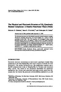
The predominant theoretical picture of solid–state and/or molecular systems involves the inhomogeneous electron gas: a set of interacting point electrons moving quantum–mechanically in the potential field of a set of atomic nuclei, which are considered to be static (the Born–Oppenheimer approximation). Solution of such models generally requires the use of approximation schemes, of which the most basic — the independent electron approximation, the Hartree theory and Hartree– Fock theory — are routinely taught to undergraduates in Physics and Chemistry courses. However, there is another approach — Density Functional Theory (DFT) — which over the last thirty years or so has become increasingly the method of choice for the solution of such problems (see Fig. 1.). This method has the double advantage of being able to treat many problems to a sufficiently high accuracy, as well as being computationally simple (simpler even than the Hartree scheme). Despite these advantages it is absent from most undergraduate and many graduate curricula with which we are familiar. We believe that this omission stems in part from the tendency of the existing books and review papers on DFT, e.g. Refs. [1–3], to follow the historical path of development of the theory. Although appropriate for a thorough treatment, this approach unnecessarily prolongs the introduction and grapples with problems which are not directly relevant to the practitioner. It is our purpose here to give a brief and self–contained introduction to density functional theory, assuming only a first course in quantum mechanics and in thermostatistics. We break with the traditional approach by relying on the analogy with thermodynamics [4]. In this formulation, the use

1000

Hartree−Fock

100 Density Functional Theory

10 1970

1975

1980

1985 year

1990

1995

FIG. 1. One indicator of the increasing use of DFT is the number of records retrieved from the INSPEC databases by searching for the keywords “density”, “functional” and “theory”. This is compared here with a similar search for keywords “Hartree” and “Fock”, which parallels the overall growth of the INSPEC databases (for any given year, approximately 0.3% of the records have the Hartree–Fock keywords).

of the density distribution as a free variable arises in a natural manner, as do more advanced concepts which are central to recent developments in the theory [5], e.g. the exchange–correlation hole and generalized compressibilities. The discussion is sufficiently detailed to provide a useful overview for the beginning practitioner, and the relatively novel point of view may also prove illuminating for those experienced researchers who are not familiar with it. We hope that the availability of such an introduc-

1

tion will encourage teachers to include a one or two hour class on DFT in courses on quantum mechanics, atomic and molecular physics, condensed matter physics, and materials science. The general theoretical framework of DFT, involving the Hohenberg–Kohn free energy FHK [n(r)], is presented in Sec. II, which for simplicity focuses on classical systems. The generalization to the quantum–mechanical electron gas is given in Sec. III, together with the discussion of the Kohn–Sham equations and of the local density approximation, which is the simplest practical approximation for the exchange–correlation energy. Various issues relating to the accuracy of this approach are discussed in Sec. IV, followed by a summary in Sec. V.

µ Ωµ

N

the temperature is in energy units (i.e. kB = 1), and the classical trace, Tr, represents the 6M –dimensional phase–space integral (the division by M ! compensates for double counting of many–body states of indistinguishable particles). It follows directly from these definitions that the expectation value of the number of particles in the system is given by a derivative of the grand potential, N = hM i = −(∂Ω/∂µ). The convexity of the thermodynamic potential [8] implies that N is a monotonically increasing function of µ. Other partial derivatives of Ω give the values of additional physical quantities, such as the entropy, S = −(∂Ω/∂T ) and the pressure P = −(∂Ω/∂V ). This may be summarized by writing dΩ = −N dµ − S dT − P dV . A basic lesson of thermodynamics is that in different contexts it is advantageous to use different ensembles. For example, in studying systems where the number of particles rather than the chemical potential is fixed, it is preferable to use the Helmholtz free energy [9], which is obtained from the grand potential Ω by
a Legendre transform: F (N, T, V ) = Ω µ(N ), T, V + µ(N )N . Here µ(N ) is no longer an independent variable, but a function of N obtained by inverting the relationship N = N (µ, V, T ) = −(∂Ω/∂µ). The derivative of F with respect to the “new” free variable N is equal to the “old” free variable µ. The derivatives with respect to the other variables are unchanged (but are taken at constant N rather than at constant µ). We thus write dF = µ dN − S dT − P dV . For the purpose of comparison with DFT, it is useful to make a variation on the inverse Legendre transform which

A. Thermodynamics: a reminder

We begin by rederiving the equations of thermodynamics from statistical mechanics [7]. Consider a classical system of M interacting particles in a container of volume V . The many–body Hamiltonian is: (1)

PM

where T = i=1 p2i /2m is the kinetic energy, and U = P i 1 Ω(µa ) + Ω(µb ) , i.e. that for the partition func2 tion one has Ξ(µc )2 < Ξ(µa )Ξ(µb ), follows directly from Eq. (3) and the inequality of the harmonic and √ xy, where x = algebraic averages, 21
(x + y) >
′ exp (M µa + M µb )/T , y = exp (M ′ µa + M µb )/T , and x 6= y. This proof generalizes to the functional situation, where v(r) replaces µ, see the appendix of M. Valiev and G.W. Fernando, “Generalized Kohn–Sham density functional theory via the effective action formalism”, preprint cond–mat/9702247. Note that the convexity or second derivative of Ω(µ) may vanish in extreme cases such as at zero temperature limit (because there only terms with x = y remain) or in the thermodynamic limit, at the point of a first–order phase transition. Mathematical consistency may be restored by restricting attention to small but finite temperatures and large but finite volumes (cf. Ref. [18]). F (N ) thus defined is not identical with that obtained by fixing the particle number — the equivalence of the canonical and grand–canonical ensembles is guaranteed only in the thermodynamic limit. However, we will later focus on the T → 0 limit in which the equivalence is regained because the fluctuations of the particle number vanish. Functionals and functional derivatives are not always familiar concepts to students, especially undergraduates, and a discussion of DFT is an excellent opportunity for them to be introduced. For our purposes one may simply regard the functional variables, n(r) and v(r) above, as defined on a dense lattice of K points rk ,

12

R

[13]

[14]

[15] [16]

[17]

[18]

[19]

[20] [21]

[22]

[23]

Fermi theory,” Rev. Mod. Phys. 34, 627–630 (1962). [24] N.H. March, “Origins: the Thomas–Fermi theory,” in Ref. [3], pp. 1–78. [25] At finite temperatures, the Fermi–Dirac distribution is used for the occupations fi of the Kohn– Sham −T S =
P∞ orbitals, and an entropic term, T i=1 fi log(fi ) + (1 − fi ) log(1 − fi ) must be included in Fni ; the approximation used for Exc [n] is also affected; see, e.g., N. Marzari, D. Vanderbilt, and M.C. Payne, “Ensemble density functional theory for ab initio molecular dynamics of metals and finite–temperature insulators,” Phys. Rev. Lett. 79, 1337–1340 (1997). [26] For completeness, we write the interacting ground–state energy E0 explicitly in terms of the Kohn–Sham eigenvalues and the density distribution:

a ground–state energy functional FL [n] + dr n(r) v(r), ˆ |Ψi, a definition which with FL [n] = minΨ→n hΨ|Tˆ + U is valid for any reasonable n(r). Whereas the thermodynamic approach used here clarifies the special role of the density distribution n(r), in Levy’s formulation one could equally well imagine other ways of constraining the search to other subspaces of the Hilbert space. P. Hohenberg and W. Kohn, “Inhomogeneous electron gas,” Phys. Rev. 136, B864–867 (1964); The generalization to a finite–temperature grand–canonical ensemble was provided almost immediately by N.D. Mermin, “Thermal properties of the inhomogeneous electron gas,” Phys. Rev. 137, A1441–1443 (1965). M.C. Payne et al., “Iterative minimization techniques for ab initio total–energy calculations: Molecular dynamics and conjugate gradients,” Rev. Mod. Phys. 64, 1045– 1097 (1992). J.D. van der Waals, Ph.D. Thesis, University of Lieden (1873). Clearly, multiple local minima occur only if −v = ∂(nf )/∂n = f + nf ′ varies nonmonotonically with n, i.e. possesses regions of negative slope. This condition is identical with the conventional one of negative compressibility, κ < 0, because κ = ∂P/∂n = (∂/∂n)(n2 ∂f /∂n) = 2nf ′ + n2 f ′′ , which is just n times the abovementioned slope (the density n is always positive). Note that these negative slopes exist only in the phenomenological model, Eq. (12); a proper statistical mechanical evaluation of the partition function would exhibit regions of phase separation instead. W. Kohn and L.J. Sham, “Self–consistent equations including exchange and correlation effects,” Phys. Rev. 140, A1133–1138 (1965). We consider small but positive temperatures, T → 0, rather than the situation at T = 0, where the function N (µ) can take only integer values and becomes discontinuous (if one insists on working at T = 0, the functionalRderivative, e.g. in Eq. (21), must be redefined so that dr δn(r) = 0). For a discussion, see e.g. J.P. Perdew, R.G. Parr, M. Levy, and J.L. Balduz, “Density– functional theory for fractional particle number: derivative discontinuities of the energy,” Phys. Rev. Lett. 49, 1691–1694 (1982). Note that this definition differs from the conventional one for exchange–correlation energy, because Fni [n] is the kinetic energy of a system of noninteracting particles with the density n(r), rather than the kinetic energy of the interacting electron system. L.H. Thomas, “Calculation of atomic fields,” Proc. Camb. Phil. Soc. 33, 542–548 (1927). E. Fermi, “Application of statistical gas methods to electronic systems,” Accad. Lincei, Atti 6, 602–607 (1927); “Statistical deduction of atomic properties,” ibid, 7, 342– 346 (1928); “Statistical methods of investigating electrons in atoms,” Z. Phys. 48, 73–79 (1928). L. Spruch, “Pedagogic notes on the Thomas–Fermi theory (and some improvements): atoms, stars, and the stability of bulk matter,” Rev. Mod. Phys. 63, 151–209 (1991). E. Teller, “On the stability of molecules in the Thomas–

E0 =

N X i=1

ǫi −

Z




dr n(r) veff (r) − v(r) +Ees [n(r)]+Exc [n(r)] .

[27] Interestingly, the work function of a metal surface is equal to that of the Kohn–Sham system. Using the fact that both ϕ(r) and vxc (r) decay as 1/r at large distances away from the system, and using the usual convention of taking v(r) and veff (r) to vanish at infinity, one finds that Eq. (19) reduces to a statement of the equality of the chemical potentials for the interacting and the Kohn– Sham system. [28] See, e.g., S.B. Nickerson, and S.H. Vosko, “Prediction of the Fermi surface as a test of density–functional approximations to the self–energy,” Phys. Rev. B 14, 4399–4406 (1976). [29] D. Mearns, “Inequivalence of the physical and Kohn– Sham Fermi surfaces,” Phys. Rev. B 38, 5906–5912 (1988). [30] G.D. Mahan, “GW approximations,” Comm. Cond. Mat. Phys. 16, 333–354 (1994). [31] O. Gunnarsson, and B.I. Lundqvist, “Exchange and correlation in atoms, molecules, and solids by the spin– density formalism,” Phys. Rev. B 13, 4274–4298 (1976). [32] E.P. Wigner, “Effects of electron interaction on the energy levels of electrons in metals,” Trans. Faraday Soc. 34, 678–685 (1938). [33] It is interesting to compare the Kohn–Sham equations with the well–known Hartree approximation. In the latter scheme each electronic orbital is calculated with a different electrostatic potential, which is due only to the other electrons, and not to the total density distribution. There exist also hybrid schemes, called “self– interaction corrected” schemes, where such different potentials are used and an extra potential vxc is included. Although such schemes have given good results for some systems (e.g. crystals with localized electrons, i.e. insulators), they do not follow the logic of either the Hartree or the DFT method. See J.P. Perdew and A. Zunger, “Self-interaction correction to density-functional approximations for many-electron systems,” Phys. Rev. B 23, 5048–5079 (1981). [34] J. Harris, “Adiabatic–connection approach to Kohn– Sham theory,” Phys. Rev. A 29, 1648–1659 (1984). [35] O. Gunnarsson, M. Jonson, and B.I. Lundqvist, “De-

13

[36]

[37]

[38]

[39]

[40]

[41]

[42]

[43]

[44]

[45]

[46] [47]

[48] [49] [50]

[51]

[52]

5684 (1990). [53] W. Kohn, Y. Meir, and D.E. Makarov, “Van der Waals energies in density functional theory,” Phys. Rev. Lett. 80, 4153-4156 (1998). [54] See, e.g., C. Speicher, R. M. Dreizler, and E. Engel, “Density functional approach to quantumhadrodynamics: Theoretical foundations and construction of extended Thomas-Fermi models,” Ann. Phys. (San Diego) 213, 312–354 (1992).

scription of exchange and correlation effects in inhomogeneous electron systems,” Phys. Rev. B 20, 3136 (1979). See, e.g., S.H. Vosko, L. Wilk, and M. Nusair, “Accurate spin–dependent electron liquid correlation energies for local spin density calculations: a critical analysis,” Can. J. Phys. 58, 1200–1211 (1980), which provides a widely–used version of ǫxc (n↑ , n↓ ). D.C. Langreth and J.P. Perdew, “Theory of nonuniform electronic systems I: Analysis of the gradient approximation and a generalization that works,” Phys. Rev. B 21, 5469–5493 (1980); J.P. Perdew and Y. Wang, “Accurate and simple density functional for the electronic exchange energy: generalized gradient approximation,” Phys. Rev. B 33, 8800–8802 (1986). J.P. Perdew et al., “Atoms, molecules, solids, and surfaces: applications of the generalized gradient approximation for exchange and correlation,” Phys. Rev. B 46, 6671–6687 (1992). For example, see the proceedings of the VIth International Conference on the Applications of Density Functional Theory. (Paris, France, 29 Aug.—1 Sept. 1995), Int. J. Quantum Chem. 61(2) (1997). A.D. Becke, “Density–functional thermochemistry III: The role of exact exchange,” J. Chem. Phys. 98, 5648– 5652 (1993); “Density–functional thermochemistry IV: A new dynamical correlation functional and implications for exact–exchange mixing,” ibid, 104, 1040–1046 (1996). R.O. Jones and O. Gunnarsson, “The density functional formalism, its applications and prospects,” Rev. Mod. Phys. 61, 689–746 (1989). M.D. Segall et al., “First principles calculation of the activity of cytochrome P450,” Phys. Rev. E 57, 4618– 4621 (1998). R. Shah, M.C. Payne, M.-H. Lee and J.D. Gale, “Understanding the catalytic behavior of zeolites — a first– principles study of the adsorption of methanol,” Science 271, 1395–1397 (1996). M.J. Rutter and V. Heine, “Phonon free energy and devil’s staircases in the origin of polytypes,” J. Phys.: Cond. Matter 9, 2009–2024 (1997). W.-S. Zeng, V. Heine and O. Jepsen, “The structure of barium in the hexagonal close-packed phase under high pressure,” J. Phys.: Cond. Matter 9, 3489–3502 (1997). F. Kirchhoff et al., “Structure and bonding of liquid Se,” J. Phys.: Cond. Matter 8, 9353–9357 (1996). R. Car and M. Parrinello, “Unified approach for molecular dynamics and density–functional theory,” Phys. Rev. Lett. 55, 2471–2474 (1985). R. McWeeny and B.T. Sutcliffe, Methods of Molecular Quantum Mechanics (Acad. Press, London, 1969). W. Kohn, “Density functional theory for systems of very many atoms,” Int. J. Quant. Chem. 56, 229–232 (1994). V.L. Moruzzi, J.F. Janak, and A.R. Williams, Calculated Electronic Properties of Metals (Pergamon, New York, 1978). G. Makov and M.C. Payne, “Periodic boundary conditions in ab initio calculations,” Phys. Rev. B 51, 4014 (1995). See, e.g., Z.Y. Zhang, D.C. Langreth, and J.P. Perdew, “Planar–surface charge densities and energies beyond the local–density approximation,” Phys. Rev. B 41, 5674–

14