Introduction . Definition of Density Gradient . Previous Work . Multilevel Gradient
Driven Dummy Fill Algorithm . Experimental Results . Conclusion and Future ...
Density Gradient Minimization with Coupling-Constrained Dummy Fill for CMP Control Huang-Yu Chen1, Szu-Jui Chou2, and Yao-Wen Chang1
1National Taiwan University, Taiwan
2Synopsys, Inc, Taiwan
NTUEE
1
Outline ․ ․ ․ ․ ․ ․
Introduction Definition of Density Gradient Previous Work Multilevel Gradient Driven Dummy Fill Algorithm Experimental Results Conclusion and Future Work
NTUEE
2
Introduction ․ Dummy fill is a general method to achieve layout uniformity before CMP (chemical-mechanical polishing)
Metals
Metals
Dummies
․ Objectives for dummy fill:
NTUEE
minimize induced coupling capacitance of dummies minimize dummy counts minimize density gradient of metal density 3
Density Gradient ․ Gradient
means the rate of change of the function value in the direction of maximum change. is generally used in solving optimization problem, such as the conjugate gradient method and the gradient descent method.
․ Density gradient of a tile
is the maximum density difference between this tile and the adjacent tiles.
․ Our work is the first work in the literature that simultaneously considers coupling constraints, dummy counts, and density gradient
NTUGIEE
4
Density Variation vs. Density Gradient ․ Density gradient is different from density variation, but both of them would affect the post-CMP thickness. Density High
Low
density variation = 0.0523 density gradient = 0.7
density variation = 0.0523 density gradient = 0.4
Considering density variation is not sufficient! NTUEE
5
Previous Work ․ Highlighted the importance of density variation
Chen et al., “Closing the Smoothness and Uniformity Gap in Area Fill Synthesis,” ISPD’02.
․ Considered wire density control during routing
Li et al., “Multilevel Full-Chip Routing with Testability and Yield Enhancement,” TCAD’07 Chen et al., “A Novel Wire-Density-Driven Full-Chip Routing System for CMP Variation Control,” TCAD’09
․ Formed a tradeoff between excessive coupling and lithography cost
Deng et al., “Coupling-Aware Dummy Metal Insertion for Lithography,” ASPDAC’07.
․ Found the maximum dummy insertion regions with no coupling violation
NTUEE
Xiang et al., “Fast Dummy-Fill Density Analysis With Coupling Constraints,” TCAD’08. 6
Previous Work: Coupling-Constrained Dummy Fill
․ CDF Algorithm presented in [Xiang et al. TCAD’08]
slots 1 2
A layout
Did not consider density gradient!
3
4
5
6
Slot partition by endpoints of segments
Coupling-free fill regions identification for each slot
Used too many dummies! Filling max # of dummies into these regions
NTUEE
7
Our Algorithm Flow Routed layout
Coupling constraints
CDF [TCAD’08] Slot-based layout
Coupling-violation-free dummy area
Slot-to-tile conversion & Density bounds computation Tile-based layout
Density upper and lower bounds
Gradient-driven multilevel dummy fill Fill result NTUEE
8
Slot-to-Tile Conversion and Density Bounds Computation
․ Convert slot-based layout to tile-based layout ․ Compute tile density bounds in each tile satisfying both coupling and foundry density rules Segment
Lower bound Bl =
Upper bound Bu =
Fill region
Further adjust the bounds according to foundry density rules
(Bl, Bu) guarantees no coupling and density rule violations in the following stages NTUEE
9
Gradient-Driven Dummy Fill Flow Routed Gradient-driven multilevel dummy fill Coupling constraints layout Multilevel dummy density analysis CDF [TCAD’08] Coarsening analysis Slot-based Coupling-violation-free layout dummy area Uncoarsening analysis Slot-to-tile conversion Density bounds computation Tile-based Density upper and layout lower bounds ILP-based dummy number assignment Gradient-driven multilevel dummy fill Fill result NTUEE
10
Multilevel Dummy Density Analysis
G2
G2
G1
G1
G0
G0 Metal Density
Coarsening (1) Gradient minimization by Gaussian smoothing (2) Density bounds update level by level NTUEE
Low
Uncoarsening High
(1) Density extraction (2) ILP-based dummy number assignment
11
Coarsening: Gradient Minimization ˆˆ = ∑ Dc ( x, y ) g ( x, y ) ․ Gaussian smoothing at tile (x,y)
Dc(x,y): original density g(x,y): weighting function =
( x − xˆˆ) 2 + ( y − y ) 2 exp(− ) 2 2 2πσ 2σ 1
0.1 0.4 0.1 0.2 0.3
0.25 0.36 0.20 0.21 0.28
Gaussian smoothing (σ=1.0)
0.2 0.4 0.4 0.3 0.2 0.3 0.3 0.2 0.2 0.1 0.1 0.1 0.2 0.1 0.3
0.27 0.36 0.35 0.28 0.26 0.24 0.25 0.24 0.20 0.18 0.17 0.19 0.23 0.19 0.27
0.2 0.2 0.4 0.3 0.4
0.22 0.25 0.35 0.27 0.34
․ Gaussian smoothing opens up a new direction for
NTUEE
density
density
gradient minimization
x
y
x
y
12
Coarsening: Density Analysis G2
G2
Gradient minimization
0.23 0.29 0.28
0.26 0.30 0.31
Average
0.26 0.30 0.32
0.28 0.30 0.32
0.22 0.25 0.28
0.27 0.30 0.31
G1 0.23 0.28 0.25
0.27 0.28 0.28
0.29 0.25 0.30
0.29 0.29 0.30
0.18 0.23 0.23
0.26 0.27 0.28
G0 0.1 0.2 0.3
0.2 0.2 0.3
0.2 0.2 0.2
0.2 0.2 0.3
0.1 0.1 0.3
0.2 0.2 0.3
NTUEE
13
Coarsening: Tile Density Bounds Update 0.4 0.4 0.4 0.4 0.4 0.4 0.4 0.4 0.4 0.2 0.2 0.3
G0
0.33
Bu(x,y) G1 0.23
0.2 0.2 0.3
Bu
=0.23+min{Bu(x,y) -Dc(x,y)} =0.23+(0.4-0.3)
0.2 0.2 0.3
Density Dc(x,y) after Gaussian smoothing
0.1 0.1 0.1 0.1 0.1 0.1 0.1 0.1 0.1
Bl(x,y)
NTUEE
0.13 Bl
=0.23-min{Dc(x,y) -Bl(x,y)} =0.23-(0.2-0.1)
Prune the value larger (smaller) than Bu (Bl) 14
Uncoarsening: Density Extraction G2
G2
Gradient minimization
0.23 0.29 0.28
0.26 0.30 0.31
Average
0.26 0.30 0.32
0.28 0.30 0.32
0.22 0.25 0.28
0.27 0.30 0.31
Density extraction
G1
G1
0.23 0.28 0.25
0.27 0.28 0.28
0.30 0.31 0.31
0.29 0.25 0.30
0.29 0.29 0.30
0.32 0.32 0.33
0.18 0.23 0.23
0.26 0.27 0.28
+0.03
G0
G0
0.1 0.2 0.3
0.2 0.2 0.3
0.2 0.2 0.2
0.2 0.2 0.3
0.1 0.1 0.3
0.2 0.2 0.3
NTUEE
0.29 0.30 0.31
0.28 0.28 0.38
+0.08
0.28 0.28 0.38 0.28 0.28 0.38
15
ILP-based Dummy Number Assignment ․ Optimally insert minimal # of dummies to satisfy the ․
desirable tile density dd in a tile For the tile with n fill regions R1,…,Rn,
minimize
∑
n
r
i =1 i
n 1 1 subject to d d a − amax ≤ ∑i =1 ai ri ≤ d d a + amax 2 2 ri ≤ ui , i = 1,, n
R1
ri: # of dummies in Ri dd: dummy density of tile a: tile area ai: area of one dummy in Ri amax: max {ai} ui: max # of dummies in Ri NTUEE
R2
u2=3 a2=4 u1=5 a1=3
amax=4
16
Experimental Setting ․ ․ ․ ․
Programming language: C++ Workstation: 2.0 GHz AMD-64 with 8GB memory ILP solver: lp_solve Parameters
Window size=3 × 3 Gaussian smoothing: σ=1.0 Foundry density lower and upper bounds: 20% and 60%
․ Test cases: MCNC and industrial Faraday benchmarks ․ Comparison with the CDFm algorithm [modified from CDF algorithm, TCAD’08] for all layers and layer 1
NTUEE
CDF algorithm: tries to insert as many dummies as possible CDFm algorithm: also honors the density lower and upper bound rules 17
Benchmarks ․ Routing results from Chen et al., ICCAD’07 Wire Density
Circuit
Size (μm×μm)
#Layer
#Segment
#Level
Mcc1
45000×39000
4
6199
Mcc2
152400×152400
4
Struct
4903×4904
Primary1
Avg.
Max
Std.
4
9.85%
47.80%
9.46%
34371
4
10.80%
54.50%
9.90%
3
10692
4
0.71%
5.19%
0.88%
7522×4988
3
6889
4
0.54%
9.10%
0.94%
Primary2
10438×6488
3
28513
4
1.23%
10.10%
1.39%
S5378
435×239
3
9816
3
8.68%
30.30%
5.60%
S9234
404×225
3
8462
3
7.43%
30.80%
5.80%
S13207
660×365
3
21891
3
8.98%
28.90%
5.53%
S15850
705×389
3
25699
3
9.76%
30.00%
5.04%
S38417
1144×619
3
64045
3
8.32%
32.10%
4.87%
S38584
1295×672
3
85931
3
9.37%
28.40%
4.55%
Dma
408.4×408.4
6
98018
5
15.60%
71.40%
16.30%
Dsp1
706.0×706.0
6
169867
5
10.70%
55.10%
13.40%
Dsp2
642.8×642.8
6
159525
5
11.00%
60.50%
13.20%
Risc1
1003.6×1003.6
6
237862
5
8.74%
58.10%
12.90%
Risc2
959.6×959.6
6
240978
5
8.82%
50.60%
11.90%
NTUEE
18
Runtime and Inserted Dummy Counts ․ Inserted dummy count is only 19% compared with CDF algorithm
․ Timing overhead is only 19%
NTUEE
CDF
Ours
Circuit #Dummy
Time (s)
#Dummy
Time (s)
Mcc1
1,262,298
160
163,821
171
Mcc2
20,117,831
7249
4,282,218
7292
Struct
9,004,650
45
159,457
72
Primary1
7,102,170
32
188,771
53
Primary2
24,897,686
428
360,221
490
S5378
269,916
21
53,527
22
S9234
230,220
14
58,230
17
S13207
657,861
73
141,723
76
S15850
721,317
99
155,336
103
S38417
2,100,467
330
248,582
337
S38584
2,460,061
518
277,747
526
Dma
1,457,877
67
321,635
101
Dsp1
3,648,742
290
1,012,893
330
Dsp2
2,815,009
189
778,375
231
Risc1
9,071,800
252
3,208,787
312
Risc2
7,235,118
396
2,626,317
446
Comp.
1.00
1.00
0.19
1.19 19
Statistics of Metal Density (MCNC) ․ The average density gradient are reduced by 70% and 59% among all layers and of layer 1, respectively CDF Analysis Algorithm Circuit
Density Gradient among Layers
Ours
Density Gradient of Layer 1
Avg.
Max
Std.
Avg.
Mcc1
7.14%
35.81%
5.87%
5.28%
Mcc2
4.40%
14.67%
2.39%
Struct
1.41%
5.75%
Primary1
2.38%
Primary2
Std.
Density Gradient of Layer 1
Avg.
Max
Std.
Avg.
Max
Std.
12.53% 12.31%
1.59%
14.42%
1.80%
1.81%
11.73%
3.62%
3.53%
8.16%
5.07%
2.23%
16.84%
2.54%
2.80%
12.07%
5.21%
1.34%
0.56%
5.67%
2.74%
0.16%
0.33%
0.07%
0.19%
0.33%
0.13%
13.09%
2.54%
1.61%
10.34%
4.60%
0.14%
0.32%
0.08%
0.17%
0.32%
0.15%
1.22%
3.97%
0.97%
0.20%
1.25%
2.44%
0.12%
0.25%
0.05%
0.14%
0.25%
0.10%
S5378
5.38%
15.88%
2.53%
5.38%
12.85%
4.37%
1.99%
10.00%
0.96%
2.18%
5.36%
1.70%
S9234
6.31%
20.79%
3.18%
6.27%
14.01%
5.52%
2.02%
8.67%
1.11%
2.25%
4.26%
1.96%
S13207
4.19%
14.62%
1.98%
3.54%
9.24%
3.61%
1.53%
7.54%
0.91%
1.49%
5.52%
1.59%
S15850
4.13%
12.50%
1.92%
3.64%
8.81%
3.43%
1.38%
9.90%
0.79%
1.36%
2.41%
1.38%
S38417
2.91%
9.32%
1.42%
2.28%
6.67%
2.68%
0.93%
9.97%
0.85%
0.89%
1.53%
1.47%
S38584
2.80%
8.97%
1.29%
2.41%
7.08%
2.34%
0.79%
8.24%
0.68%
0.79%
1.38%
1.18%
Comp.
1.00
1.00
1.00
1.00
1.00
1.00
0.30
0.56
0.39
0.41
0.47
0.38
NTUEE
Max
Density Gradient among Layers
20
Statistics of Metal Density (Faraday) ․ The average density gradient are reduced by 40% and 91% among all layers and of layer 1, respectively CDF Analysis Algorithm Circuit
Density Gradient among Layers
Ours
Density Gradient of Layer 1
Density Gradient among Layers
Density Gradient of Layer 1
Avg.
Max
Std.
Avg.
Max
Std.
Avg.
Max
Std.
Avg.
Max
Std.
Dma
3.39%
19.50%
3.30%
1.77%
10.22%
9.01%
2.23%
21.45%
3.10%
0.60%
1.01%
8.57%
Dsp1
2.90%
24.33%
3.69%
2.87%
24.33%
9.03%
1.49%
20.08%
2.50%
0.14%
0.57%
6.95%
Dsp2
2.66%
26.81%
3.62%
2.85%
26.81%
8.88%
1.24%
17.27%
1.97%
0.14%
0.59%
5.53%
Risc1
2.66%
21.15%
3.52%
2.74%
18.79%
8.62%
1.77%
21.15%
3.12%
0.14%
0.40%
8.62%
Risc2
2.98%
26.49%
3.92%
2.67%
17.95%
9.64%
2.02%
26.49%
3.57%
0.15%
0.45%
9.88%
Comp.
1.00
1.00
1.00
1.00
1.00
1.00
0.60
0.90
0.79
0.09
0.03
0.88
․ Overall comparison (MCNC+Faraday) CDF Analysis Algorithm Circuit
Comp.
Density Gradient among Layers
Ours
Density Gradient of Layer 1
Density Gradient among Layers
Density Gradient of Layer 1
Avg.
Max
Std.
Avg.
Max
Std.
Avg.
Max
Std.
Avg.
Max
Std.
1.00
1.00
1.00
1.00
1.00
1.00
0.37
0.66
0.51
0.32
0.31
0.53
NTUEE
21
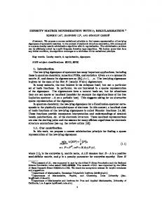
Comparison of S5378 Layer 1 Filling Results CDFm algorithm Metal density = 27.15% Fill inserted = 100%
wires fills
Ours Metal density = 21.97% Fill inserted = 20%
NTUEE
22
Conclusions and Future Work ․ Presented an effective and efficient dummy fill algorithm considering both gradient minimization and coupling constraints
Reduced 63% of density gradient among all layers Saved 91% dummy counts
․ Gaussian smoothing is effective for gradientminimization dummy fill
Point out a new research direction on this topic
․ Future work: simultaneously gradient and coupling capacitance optimization
NTUEE
23
Conclusions and Future Work ․ A dummy fill algorithm considering both gradient minimization and coupling constraints
․ Achieve more balanced metal density distribution with
Q&A
fewer dummy features and an acceptable timing overhead
Thank You!
․ Future work: integration of gradient minimization and coupling constraints
NTUEE
Simultaneously minimize the gradient and the coupling capacitance
24