Alastair Beresford and Robert Harle have been of great help by providing ... opers late in a software engineering projectâmany new lines of ..... on the desk of the user, and highlighting active real-world devices such as a ringing phone. ..... capture are cheap and ubiquitousâespecially given their recent appearance on ...
Technical Report
UCAM-CL-TR-686 ISSN 1476-2986
Number 686
Computer Laboratory
Dependable systems for Sentient Computing Andrew C. Rice
May 2007
15 JJ Thomson Avenue Cambridge CB3 0FD United Kingdom phone +44 1223 763500 http://www.cl.cam.ac.uk/
c 2007 Andrew C. Rice
Technical reports published by the University of Cambridge Computer Laboratory are freely available via the Internet: http://www.cl.cam.ac.uk/techreports/ ISSN 1476-2986
Abstract Dependable Systems for Sentient Computing Andrew Rice Computers and electronic devices are continuing to proliferate throughout our lives. Sentient Computing systems aim to reduce the time and effort required to interact with these devices by composing them into systems which fade into the background of the user’s perception. Failures are a significant problem in this scenario because their occurrence will pull the system into the foreground as the user attempts to discover and understand the fault. However, attempting to exist and interact with users in a real, unpredictable, physical environment rather than a wellconstrained virtual environment makes failures inevitable. This dissertation describes a study of dependability. A dependable system permits applications to discover the extent of failures and to adapt accordingly such that their continued behaviour is intuitive to users of the system. Cantag, a reliable marker-based machine-vision system, has been developed to aid the investigation of dependability. The description of Cantag includes specific contributions for marker tracking such as rotationally invariant coding schemes and reliable back-projection for circular tags. An analysis of Cantag’s theoretical performance is presented and compared to its real-world behaviour. This analysis is used to develop optimised tag designs and performance metrics. The use of validation is proposed to permit runtime calculation of observable metrics and verification of system components. Formal proof methods are combined with a logical validation framework to show the validity of performance optimisations.
4
Contents List of Figures
9
Acknowledgements
13
Publications
14
1
Introduction
15
1.1
Dependable Computing . . . . . . . . . . . . . . . . . . . . . . . . . . . . . .
17
1.1.1
Existing technologies . . . . . . . . . . . . . . . . . . . . . . . . . . .
17
1.1.2
Engineering for dependability . . . . . . . . . . . . . . . . . . . . . .
17
1.1.3
Algorithmic dependability . . . . . . . . . . . . . . . . . . . . . . . .
18
1.1.4
Runtime dependability . . . . . . . . . . . . . . . . . . . . . . . . . .
18
2
Related Work
19
2.1
Supporting Sentient Applications . . . . . . . . . . . . . . . . . . . . . . . . .
19
2.1.1
Operating environment . . . . . . . . . . . . . . . . . . . . . . . . . .
19
2.1.2
Coverage and boundaries . . . . . . . . . . . . . . . . . . . . . . . . .
20
2.1.3
Types of location information . . . . . . . . . . . . . . . . . . . . . .
21
2.1.4
Information delivery . . . . . . . . . . . . . . . . . . . . . . . . . . .
22
2.1.5
Direction of observation . . . . . . . . . . . . . . . . . . . . . . . . .
23
2.1.6
Search constraints . . . . . . . . . . . . . . . . . . . . . . . . . . . .
23
2.1.7
Statefulness . . . . . . . . . . . . . . . . . . . . . . . . . . . . . . . .
24
2.1.8
Sensing interface . . . . . . . . . . . . . . . . . . . . . . . . . . . . .
25
2.1.9
Calibration . . . . . . . . . . . . . . . . . . . . . . . . . . . . . . . .
35
2.2
Uncertainty in Location Information . . . . . . . . . . . . . . . . . . . . . . .
36
2.3
Fault Tolerant Systems . . . . . . . . . . . . . . . . . . . . . . . . . . . . . .
38
2.3.1
39
Hardware failure . . . . . . . . . . . . . . . . . . . . . . . . . . . . . 5
2.4 3
2.3.2
Redundancy . . . . . . . . . . . . . . . . . . . . . . . . . . . . . . . .
40
2.3.3
Fault tree analysis . . . . . . . . . . . . . . . . . . . . . . . . . . . .
41
2.3.4
State dependent analysis . . . . . . . . . . . . . . . . . . . . . . . . .
41
2.3.5
Software . . . . . . . . . . . . . . . . . . . . . . . . . . . . . . . . .
42
Summary . . . . . . . . . . . . . . . . . . . . . . . . . . . . . . . . . . . . .
43
A Platform For Investigating Dependability
45
3.1
Design Goals . . . . . . . . . . . . . . . . . . . . . . . . . . . . . . . . . . .
45
3.2
Machine Vision Systems . . . . . . . . . . . . . . . . . . . . . . . . . . . . .
46
3.3
Fundamentals of Tag Design . . . . . . . . . . . . . . . . . . . . . . . . . . .
47
3.3.1
Data coding . . . . . . . . . . . . . . . . . . . . . . . . . . . . . . . .
47
3.3.2
Tag shape . . . . . . . . . . . . . . . . . . . . . . . . . . . . . . . . .
49
Image Processing Pipeline . . . . . . . . . . . . . . . . . . . . . . . . . . . .
52
3.4.1
Entity abstraction . . . . . . . . . . . . . . . . . . . . . . . . . . . . .
52
3.4.2
Image acquisition . . . . . . . . . . . . . . . . . . . . . . . . . . . . .
54
3.4.3
Thresholding . . . . . . . . . . . . . . . . . . . . . . . . . . . . . . .
54
3.4.4
Contour following . . . . . . . . . . . . . . . . . . . . . . . . . . . .
58
3.4.5
Camera distortion correction . . . . . . . . . . . . . . . . . . . . . . .
58
3.4.6
Shape fitting . . . . . . . . . . . . . . . . . . . . . . . . . . . . . . .
59
3.4.7
Transformation . . . . . . . . . . . . . . . . . . . . . . . . . . . . . .
60
Dependable Coding . . . . . . . . . . . . . . . . . . . . . . . . . . . . . . . .
62
3.5.1
Rotational invariance . . . . . . . . . . . . . . . . . . . . . . . . . . .
63
3.5.2
Tag coding abstraction . . . . . . . . . . . . . . . . . . . . . . . . . .
65
3.5.3
Coding schemes . . . . . . . . . . . . . . . . . . . . . . . . . . . . .
66
3.5.4
Asymmetric tags . . . . . . . . . . . . . . . . . . . . . . . . . . . . .
68
3.5.5
Evaluation . . . . . . . . . . . . . . . . . . . . . . . . . . . . . . . .
69
Back-Projection for Circular Tags . . . . . . . . . . . . . . . . . . . . . . . .
71
3.6.1
Algorithm description . . . . . . . . . . . . . . . . . . . . . . . . . .
71
3.6.2
Evaluation . . . . . . . . . . . . . . . . . . . . . . . . . . . . . . . .
75
3.6.3
Resolving pose ambiguity . . . . . . . . . . . . . . . . . . . . . . . .
75
Summary . . . . . . . . . . . . . . . . . . . . . . . . . . . . . . . . . . . . .
77
3.4
3.5
3.6
3.7
6
4
5
Algorithmic Dependability
79
4.1
Specifying Performance . . . . . . . . . . . . . . . . . . . . . . . . . . . . . .
79
4.2
Features of the Camera Model . . . . . . . . . . . . . . . . . . . . . . . . . .
80
4.3
Sample Distance . . . . . . . . . . . . . . . . . . . . . . . . . . . . . . . . .
82
4.3.1
Circular tag design . . . . . . . . . . . . . . . . . . . . . . . . . . . .
84
4.3.2
Comparing square and circular tags . . . . . . . . . . . . . . . . . . .
90
4.3.3
Error-correcting coding schemes . . . . . . . . . . . . . . . . . . . . .
91
4.3.4
Implications for system deployment . . . . . . . . . . . . . . . . . . .
92
4.4
Sample Error . . . . . . . . . . . . . . . . . . . . . . . . . . . . . . . . . . .
93
4.5
Sample Strength . . . . . . . . . . . . . . . . . . . . . . . . . . . . . . . . . .
94
4.5.1
Estimated sample strength . . . . . . . . . . . . . . . . . . . . . . . .
95
4.5.2
Real-world tag reading performance . . . . . . . . . . . . . . . . . . .
97
4.5.3
Summary . . . . . . . . . . . . . . . . . . . . . . . . . . . . . . . . .
99
4.6
Location Accuracy . . . . . . . . . . . . . . . . . . . . . . . . . . . . . . . . 101
4.7
Achieving Algorithmic Dependability . . . . . . . . . . . . . . . . . . . . . . 103
4.8
Summary . . . . . . . . . . . . . . . . . . . . . . . . . . . . . . . . . . . . . 104
Runtime Dependability
107
5.1
Runtime Faults in Sentient Computing . . . . . . . . . . . . . . . . . . . . . . 107
5.2
Exploiting Asymmetric Computation . . . . . . . . . . . . . . . . . . . . . . . 108 5.2.1
Negative validation . . . . . . . . . . . . . . . . . . . . . . . . . . . . 109
5.3
Expressing Validation Requirements . . . . . . . . . . . . . . . . . . . . . . . 109
5.4
A Validation Architecture for Cantag . . . . . . . . . . . . . . . . . . . . . . . 111
5.5
A Validation Reasoning Engine . . . . . . . . . . . . . . . . . . . . . . . . . . 112
5.6
5.7
5.5.1
Implementing the check predicates . . . . . . . . . . . . . . . . . . . . 115
5.5.2
The validation process and costs . . . . . . . . . . . . . . . . . . . . . 115
5.5.3
Improving performance . . . . . . . . . . . . . . . . . . . . . . . . . 116
Application-Oriented Validation . . . . . . . . . . . . . . . . . . . . . . . . . 121 5.6.1
The LAST predicate . . . . . . . . . . . . . . . . . . . . . . . . . . . 123
5.6.2
Entry events . . . . . . . . . . . . . . . . . . . . . . . . . . . . . . . . 123
Validation for the Active Bat system . . . . . . . . . . . . . . . . . . . . . . . 125 5.7.1
Improving performance for the LAST predicate . . . . . . . . . . . . . 127
5.7.2
Ensuring system safety . . . . . . . . . . . . . . . . . . . . . . . . . . 129
5.8
Usage Modes . . . . . . . . . . . . . . . . . . . . . . . . . . . . . . . . . . . 131
5.9
Implementation Considerations . . . . . . . . . . . . . . . . . . . . . . . . . . 132 5.9.1
Validating historical events . . . . . . . . . . . . . . . . . . . . . . . . 133
5.10 Summary . . . . . . . . . . . . . . . . . . . . . . . . . . . . . . . . . . . . . 134 7
6
Conclusion
135
6.1
Investigation Platform . . . . . . . . . . . . . . . . . . . . . . . . . . . . . . . 135
6.2
Performance Metrics . . . . . . . . . . . . . . . . . . . . . . . . . . . . . . . 136
6.3
Validation . . . . . . . . . . . . . . . . . . . . . . . . . . . . . . . . . . . . . 136
6.4
Future Work . . . . . . . . . . . . . . . . . . . . . . . . . . . . . . . . . . . . 137
6.5
Summary . . . . . . . . . . . . . . . . . . . . . . . . . . . . . . . . . . . . . 137
References
139
8
Figures 1.1
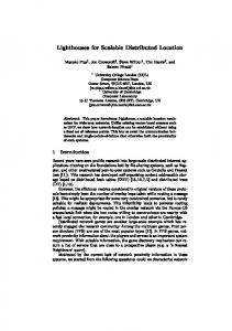
Percentage of households with electronic devices in the UK . . . . . . . . . . .
15
2.1
The SPIRIT map application showing computer-visible regions . . . . . . . . .
22
2.2
Position error in the Active Bat system due to multipath signals . . . . . . . . .
29
2.3
Relative spectral emissions from selected light sources . . . . . . . . . . . . .
30
2.4
Accuracy and precision of location estimates . . . . . . . . . . . . . . . . . .
36
2.5
Location expressed as a Probability Density Function . . . . . . . . . . . . . .
37
2.6
The bathtub curve for the probability of hardware failure . . . . . . . . . . . .
39
3.1
MBV Systems using square tag designs . . . . . . . . . . . . . . . . . . . . .
48
3.2
MBV Systems using circular tag designs . . . . . . . . . . . . . . . . . . . . .
48
3.3
Ambiguous interpretations for the pose of a circular tag . . . . . . . . . . . . .
51
3.4
Tag design terminology . . . . . . . . . . . . . . . . . . . . . . . . . . . . . .
51
3.5
The three generalised circular tag designs provided in Cantag . . . . . . . . . .
51
3.6
A simple implementation of type-lists in C++ . . . . . . . . . . . . . . . . . .
53
3.7
The ComposedEntity class . . . . . . . . . . . . . . . . . . . . . . . . . . . .
53
3.8
Inheritance diagram for an example ComposedEntity . . . . . . . . . . . . . .
54
3.9
Noise sources in images captured from CCD arrays . . . . . . . . . . . . . . .
55
3.10 Photon shot noise in equalised low-illumination images . . . . . . . . . . . . .
56
3.11 Optical illusion in colour interpretation . . . . . . . . . . . . . . . . . . . . . .
56
3.12 Thresholding under varying lighting conditions . . . . . . . . . . . . . . . . .
57
3.13 Thresholding images taken in low illumination conditions . . . . . . . . . . . .
57
3.14 Perspective effects on the TransformEllipseLinear algorithm . . . . . . . . . . .
61
3.15 Large payloads are susceptible to perspective errors . . . . . . . . . . . . . . .
61
3.16 Reading a circular tag non-invariantly or invariantly . . . . . . . . . . . . . . .
64
3.17 Reading a square tag in a rotationally invariant manner . . . . . . . . . . . . .
64
3.18 The central datacell is unused if the tag has an odd number of cells . . . . . . .
65
9
3.19 The Independent Chunk Code applied to a tag with large symbols . . . . . . .
67
3.20 Data-carrying capabilities of the evaluated coding schemes . . . . . . . . . . .
69
3.21 Error rates for the evaluated circular tag designs . . . . . . . . . . . . . . . . .
70
3.22 Error rates for the evaluated square tag designs . . . . . . . . . . . . . . . . .
71
3.23 Comparing TransformEllipseLinear to TransformEllipseFull . . . . . . . . . . .
75
3.24 Tag decoding performance of square and circular tags . . . . . . . . . . . . . .
76
4.1
The error in the tag’s normal vector is bimodal . . . . . . . . . . . . . . . . . .
80
4.2
Tag size is inversely proportional to distance from the camera . . . . . . . . . .
81
4.3
Full tag sizes for a number of example camera configurations . . . . . . . . . .
81
4.4
Tag size with fixed orientation for positions along a ray . . . . . . . . . . . . .
82
4.5
Sample distances for three example tags . . . . . . . . . . . . . . . . . . . . .
83
4.6
Analogy to the Nyquist-Shannon sampling limit . . . . . . . . . . . . . . . . .
83
4.7
Pixel aliasing affect on minimum sample distance . . . . . . . . . . . . . . . .
84
4.8
Approximating the original TRIP tag design . . . . . . . . . . . . . . . . . . .
84
4.9
TRIP tag interpolated tag size for increasing payload size . . . . . . . . . . . .
85
4.10 Tangential and radial size calculation . . . . . . . . . . . . . . . . . . . . . . .
86
4.11 Interpolated tag size of CircleInner tags against payload size . . . . . . . . . .
89
4.12 Comparing CircleInner tags with the remaining circular designs . . . . . . . .
89
4.13 Comparing CircleInner and Square tags . . . . . . . . . . . . . . . . . . . . .
90
4.14 The effect of position and pose on interpolated tag size . . . . . . . . . . . . .
91
4.15 The number of unreadable datacells for selected tag inclinations . . . . . . . .
92
4.16 The required tag size, per datacell, for one pixel of sample distance . . . . . . .
93
4.17 Sample error between the ideal and estimated sample points . . . . . . . . . .
93
4.18 Maximum sample error from FitEllipseLS and FitEllipseSimple . . . . . . . . .
94
4.19 Sample strength of FitEllipseLS and FitEllipseSimple . . . . . . . . . . . . . .
95
4.20 Approximation Error when estimating Sample Strength . . . . . . . . . . . . .
96
4.21 Cumulative Error for the Estimated Sample Strength . . . . . . . . . . . . . .
98
4.22 Experimental Setup for real-world testing of Cantag . . . . . . . . . . . . . . .
99
4.23 Sample Strength Estimates using real-world data . . . . . . . . . . . . . . . . 100 4.24 Real-world and simulated location error across processing pipelines . . . . . . 102 5.1
Functional diagram of a Cantag processing pipeline . . . . . . . . . . . . . . . 111
5.2
Inference rules for validation in Cantag . . . . . . . . . . . . . . . . . . . . . 113 10
5.3
Validation rules for Cantag (Prolog clauses) . . . . . . . . . . . . . . . . . . . 114
5.4
System validation (Prolog clauses) . . . . . . . . . . . . . . . . . . . . . . . . 115
5.5
An example validation session for Cantag . . . . . . . . . . . . . . . . . . . . 116
5.6
The number of calls to positive and negative checking functions . . . . . . . . 117
5.7
Classification of the computation costs of the checking function . . . . . . . . 118
5.8
Early rejection of candidate entities reduces validation costs . . . . . . . . . . 120
5.9
Negative validation rules for the CONT selection predicate . . . . . . . . . . . 122
5.10 Inference rules for LASTp . . . . . . . . . . . . . . . . . . . . . . . . . . . . 123 5.11 Validation of CONT and EXCL (Prolog clauses) . . . . . . . . . . . . . . . . 124 5.12 Implementation of LAST (Prolog clauses) . . . . . . . . . . . . . . . . . . . . 124 5.13 Functional diagram of the Active Bat system . . . . . . . . . . . . . . . . . . . 125 5.14 Inference rules for validation in the Active Bat System . . . . . . . . . . . . . 126 5.15 Validation inference rules for the ID predicate . . . . . . . . . . . . . . . . . . 127 5.16 Specification of validity proof for (LAST∗) and (LAST∗2 ) . . . . . . . . . . . 129 5.17 Proof of soundness for the LAST∗ predicates (Isabelle/HOL) . . . . . . . . . . 130 5.18 Proof of validity for the implementation of SID (Isabelle/HOL) . . . . . . . . . 131
11
12
Acknowledgements Many thanks are due to my supervisor Andy Hopper for his direction, insights, and guidance. I am grateful to Alan Mycroft for his acute observations and suggestions particularly in regard to C++ programming techniques, the information-theoretic limits of Cantag, and theorem proving. Alastair Beresford and Robert Harle have been of great help by providing implementations for various parts of Cantag such as the eigenvector solving routine, and algorithms for backprojection of square tags. Rotational invariance for tag coding arose from discussions with Christopher Cain. I am further indebted to him for the development and implementation of the Structured Cyclic Code (SCC) coding scheme. Further thanks go to my colleagues David Cottingham, Jon Davies, John Fawcett, Brian Jones, Matthew Parkinson, Tom Ridge, Richard Sharp, Eben Upton, and Ian Wassell for their academic guidance and proof-reading. Personal thanks go to Ewan Mellor and Cheryl O’Rourke for their support; to Paula Buttery for her love and companionship; and to my parents Victor and Lindsay. This thesis was examined by Professor Gudrun Klinker and Professor Peter Robinson. I thank them for their time and their comments. I gratefully acknowledge the financial support of the EPSRC.
13
Publications A number of the contributions presented in this work have appeared in the following publications: • Andrew Rice, Christopher Cain and John Fawcett. Dependable Coding for Fiducial Tags. In Proceedings of the 2nd Ubiquitous Computing Symposium, pages 155–163, 2004. • Andrew Rice, Christopher Cain and John Fawcett. Dependable Coding for Fiducial Tags (Extended Version). In Ubiquitous Computing Systems, LNCS 3598, pages 259–274, 2004. • Andrew Rice and Robert Harle. Evaluating Lateration-Based Positioning Algorithms for Fine-Grained Tracking. In Joint Workshop on Foundations of Mobile Computing (DIALM-POMC), pages 54–61, 2005. • Andrew C Rice, Alastair R Beresford and Robert K Harle. Cantag: an open source software toolkit for designing and deploying marker-based vision systems. In Fourth Annual IEEE International Conference on Pervasive Computer and Communications (PerCom), pages 12–21, 2006. • Andrew C Rice and Alastair R Beresford. Dependability and Accountability for Contextaware Middleware Systems. In Workshop on Middleware Support for Pervasive Computing Workshop (PerWare), pages 378–382, 2006. • Andrew C Rice, Robert K Harle and Alastair R Beresford. Analysing fundamental properties of marker-based vision system designs. In Pervasive and Mobile Computing, 2(4):453–471, 2006.
14
Chapter 1 Introduction Computers and electronic devices are continuing to proliferate throughout our lives. The time and effort required to control or interact with these devices is increasing with their number and heterogeneity. Our surroundings are burgeoning with electronic devices such as television sets, Personal Video Recorders (PVRs),control systems for central heating, microwave ovens, and in-car satelliteassisted navigation units. The number of mobile devices is also increasing. Examples of these include mobile telephones, digital cameras, and digital music players. Figure 1.1 shows evidence of these trends at the national level in the United Kingdom [52]. Communication between devices is becoming commonplace: radio and infrared networking capabilities are ubiquitous in mobile telephones; digital cameras can connect directly to personal computers; and televisions (and refrigerators) are now connected to the Internet. Acquisition of a new device combinatorially increases the complexity of our situation because it may potentially interact with all our existing devices. This is analogous to the problem of adding developers late in a software engineering project—many new lines of communication are created for each addition [24, Chapter 2]. The ultimate goal of this work is to reduce the strain on users by minimising the cognitive load of using electronic devices. This complements the vision of Ubiquitous Computing [148] which aims to create technologies that fade into the background.
Percentage of Households
100
Microwave CD Player Mobile Telephone Home Computer VCR Internet Connection
80 60 40 20 0 1994
1996
1998
2000
2002
2004
Year
Figure 1.1: Percentage of households with electronic devices in the UK 15
Research into Sentient Computing seeks to achieve this goal by shifting the onus of understanding from user to machine [75]. Machines which understand their users should be easier to use than current devices and might ultimately require no direct input at all. Currently, applications operate in a virtual environment inside the computer and we interact with them using abstract control devices such as keyboards and mice. Sentient Computing seeks to move this virtual, abstract interface into our physical, real-world environment. This is broadly in-line with the goal of Proactive Computing [135] which aims for computer systems to: 1) get physical through the use of sensors to achieve coupling with the environment; 2) get real by safely and rapidly responding to external stimuli; and 3) get out by moving human operators above the operating loop. One technique for interacting with users in the physical environment is to make applications and devices context-aware. Numerous forms of context exist that an application might utilise. Four of the most important of these are location, identity, activity, and time [40]. Substantial progress has been made towards context-aware interaction. Location information has received particular attention. At the lowest level, myriad systems have been developed for collecting location information with differing degrees of accuracy and precision. This information has been used by applications directly for location cues, and also to infer other forms of context such as identity [18] and activity [67]. Research into middleware, which run on top of location systems, has developed concepts such as spatial call-backs which assist applications running on low resource platforms by providing asynchronous notification when an event of interest occurs [2]. At the top level, many applications have been developed which exploit this information. Sentient Computing systems are extremely failure sensitive. From a conceptual standpoint it is impossible for the system to become invisible its users observe an appreciable rate of failures occurring. Due to its pervasive nature, any attempted deployment of Sentient Computing is likely to be thwarted by failures because users will not trust a fragile system. In addition to being failure sensitive, Sentient Computing systems are also failure prone. This is because, by definition, these systems are attempting to exist and interact with users in a real, unpredictable, physical environment rather than a well-constrained virtual environment. The conventional engineering approach to improving systems of this nature is to reduce the failure rate using fault tolerant hardware and software techniques. These techniques are also applicable within Sentient Computing systems but their application must not detract from other aspects of the system: common goals for devices and systems such as miniaturisation or mobility impose size and power consumption constraints which limit the efficacy of fault tolerant engineering. A dependable system can provide, at any time, a specification of current system performance and status. Applications are able to determine when a failure occurs and adapt accordingly. The system’s dependability is the proportion of time that the actual service level matches the advertised service level. Dependability aims to reduce the failure sensitivity of Sentient Computing by enabling applications to adapt to faults and continue to operate to the best possible extent. 16
1.1
Dependable Computing
The contribution embodied in this work is a structured approach to implementing dependable systems for Sentient Computing. Specifically, this consists of:
• implementation of a location system with the specific goal of supporting dependability; • particular improvements to the robustness of machine vision algorithms used in location systems; • a process for analysing the performance of a location system and deriving performance metrics; • integration of these metrics with tests for software implementation errors and algorithmic errors using validation.
The scope of this work is the support of applications for Sentient Computing. A practical and pragmatic approach is adopted based on the current capabilities and performance of devices. The intent herein is not to build the most accurate or most highly performing (by some metric) system, but to construct systems with understandable, predictable behaviour whilst still meeting the goals of Sentient Computing.
1.1.1 Existing technologies Chapter 2 presents a top-down survey of Sentient Computing. It begins with an examination of high-level application requirements, progressing on to the features and behaviours of location systems. Particular attention is paid to the reliability challenges presented at each stage. By considering the needs of applications, this chapter aids the identification of design goals for dependable systems. Consideration of available technologies and current approaches motivates design choices made later in this work.
1.1.2 Engineering for dependability Chapter 3 describes the provision of dependability by working upwards from the low-level sensors in a system. This is realised through the development of a dependability-oriented location system: the creation of Cantag, a marker-based machine-vision location system, is presented. Testing Cantag using an integrated test harness highlighted algorithmic problems with current marker-based vision techniques—these problems are rectified and the performance improvements are demonstrated. 17
1.1.3 Algorithmic dependability Chapter 4 presents an investigation into the theoretical behaviour of Cantag. The goal is to define metrics which describe the current performance of the system. An information-theoretic argument is used to bound the best performance of this class of location system. The benefit of this high-level analysis is demonstrated through design-optimisation for circular marker tags. Results from simulation are examined to compare the performance and stability of candidate image processing algorithms. Further metrics for system behaviour are developed. Real-world results from Cantag are presented and compared to the simulated data. A dependable tag design and processing pipeline is identified whose simulated performance correctly predicts its real-world behaviour.
1.1.4 Runtime dependability Chapter 5 investigates the concept of validation for data in a dependable system. Many of the computations in Cantag (and other Sentient Computing systems) are asymmetric. This means that the forward computation of the result from the input data is computationally more expensive than the backward computation required to check that the result is consistent with the input data. Validation is particularly useful in a dependable system to protect against implementation and algorithmic errors within the system. Validation also integrates the previously identified metrics for system performance by using them as the basis for additional acceptance tests. An example implementation of validation is presented and evaluated using logic programming (Prolog) extended by external predicates for interacting with the location system. The cost of validating particular pieces of context as required by an application is examined and techniques for reducing this cost are demonstrated.
18
Chapter 2 Related Work 2.1
Supporting Sentient Applications
The construction of a dependable application cannot proceed without first providing a dependable infrastructure. This infrastructure includes any sources of context used by the application, and additional support functionality such as facilities provided by a middleware. This section presents various classifications of applications and sensor systems in order to codify the needs of sentient applications and the features provided by existing sentient infrastructure components. Location systems are of particular interest because they provide a primary source of context [40] for many applications and so are most likely to form a key part of future dependable systems.
2.1.1 Operating environment Office environments have been a common focus for Sentient Computing. A telephone receptionist’s aid based on room-level location was an early example [144]. More fine-grained location information has also been exploited in this environment to provide real-time maps and to automatically select cameras for videoing employees and visitors as they move around [145, Chapter 9]. Other targeted environments have included museums and exhibition halls in which researchers sought to provide additional information to visitors as they arrived at a particular exhibit [33]. Another study considered the hospital environment and provided a messaging system which can address users by role, location, and time [99]. Context-aware applications have also been deployed in the home using cues from the occupants’ locations for smart control of media devices and lighting [84]. Outdoor applications include city-wide location-based gaming where virtual players are chased by runners in the real world [15]. Drishti is a navigation system for the blind which is suitable for both indoor and outdoor operation through handover between different location technologies [112]. Different environments present different challenges for a location system. Signal propagation is affected by the structure of the space: small offices limit propagation more than open-plan 19
spaces. Occupants’ movement patterns differ between environments. In outdoor spaces people might move purposefully towards a destination or browse more casually whereas in office environments an occupant might primarily travel between their desk and the provided amenities. The acceptability of any location sensing is also environment dependent: users who participate at work may well be loathe to wear marker tags (or even to be tracked at all) at home. Systems operating in outdoor environments must cope with extremes of temperature, lighting, and humidity produced whereas indoor environments benefit from some measure of protection from the weather. Also, useful infrastructure (such as power and network wiring) which might be exploited by a location system is more common within buildings rather than in outdoor environments.
2.1.2 Coverage and boundaries Applications place widely ranging requirements on the coverage of a location system. The Invisible Train application uses a camera and a handheld computer (PDA) to present an augmented view of the world [141]. Only a limited coverage area is required because the acquired image is shown with annotations on a small PDA screen. Conversely, the ActiveMap application provides a visualisation of the (room-level) locations of users [95]. Coverage of a significant number of offices is necessary for this application to be useful. A location system’s boundaries are also an important consideration. A system is said to be boundary transparent if a user is not required to take any action when tracking commences. Users may enter and leave the coverage areas of boundary transparent systems without special action. Boundary transparency increases in importance as the amount of time the user spends within the system decreases. This is often correlated with coverage area: smaller coverage areas imply reduced residency times and thus increased requirement for boundary transparency. The Polhemus Liberty tracker1 is a magnetic tracker with very high accuracy over short ranges: 0.0038 mm RMS error within 30 cm of the field source. However, its use of a tethered stylus (which cannot leave the system at all) makes it boundary opaque. The Active Badge system consists of mobile badges worn by users. The badges periodically broadcast a unique identifier over an infrared channel [144]. This is decoded by room-level receivers and passed to a central location service. Reflections from walls and furniture make the infrared signal likely to reach the receiver without requiring direct line-of-sight. This is an example of a boundary transparent system because the tags carried by the user are automatically acquired by the system when the user enters the room. The camera-based tracking system used for the Invisible Train is boundary transparent because the tracked objects (fiducial marker tags) may enter and leave the field-of-view without hindrance. The application would become infeasible if this were not the case. It is only acceptable for a location system to be boundary opaque if users’ residency times within the system are of substantial duration. 1
http://www.polhemus.com/
20
2.1.3 Types of location information Applications typically expect a range of contextual data in addition to location information. These may include the identity of the locatable object and time of sighting. The form of these data vary according to the application’s needs. Desktop teleporting permits a user to move their desktop onto the currently visible machine [118]. This requires containment information i.e. which machine is contained within the spatial region which represents the user’s field-of-view. The user’s ’aura’ is another commonly used term with this meaning. This type of information is referred to as symbolic information. Symbolic information has no spatial grounding. Interpretation of these symbols often requires a mapping from the symbolic identifier to the current frame of reference. For example, the symbolic identifiers of receivers in the Active Badge system are mapped onto the perimeter of the relevant room in the Euclidean space which describes the building. Steerable interfaces have been considered by researchers as a means of intuitively positioning the interface to an application [108]. Examples include a reminder note application positioned on the desk of the user, and highlighting active real-world devices such as a ringing phone. These applications require a different kind of positioning information known as metric information. The term metric information is very superficially related to a metric space in mathematics which defines a set where there is a notion of distance between the elements. Analogously, metric location information has the same property. The Active Bat system calculates location information from time-of-flight estimates of an ultrasonic pulse emitted by a mobile Bat [146]. This produces metric location information in a Euclidean coordinate frame. The Navstar (Navigation Satellite and Ranging) GPS (Global Positioning System) produces metric location in the WGS84 coordinate frame from the differences between arrival times of signals from timesynchronised satellites in known orbits [58]. The classification of symbolic or metric information is applicable to other forms of context provided by the location system. Systems such as the Active Badge system produce symbolic information for the identifier of the beacon and the receiver. The time of the sighting is metric information because the distance in time between two sightings is a useful concept. In the Active Bat system the identifier of the Bat itself is symbolic information whereas the time of the sighting, and the location and orientation of the Bat, are metric information. A further example is the Active Floor which measures the Ground Reaction Force (GRF) at the corners of floor tiles using load sensors [1]. A Hidden Markov Model (HMM) is used to infer the identity of a walker through gait classification. The time of the measurement and location (in terms of which tiles are occupied) of the user are both metric information. In this case the identity of the user is also metric information. Classification of the user can be viewed as taking part in a space of classification features in which there are regions representing the learned classification for each individual user. The estimate of identity is a point within this space. This final example exemplifies that the definition of distance in a metric system should contain some useful meaning. This is evidently true for coordinates and time. Furthermore, for the identity of a user in the Active Floor the similarity between users (in terms of gait or other features) is physically relevant. However, in the Active Bat system examining the similarity between the symbolic identifiers of two Bats is not particularly useful. 21
Figure 2.1: The SPIRIT map application showing computer-visible regions In order to facilitate its application to quantities such as time, the term metric is preferred over alternatives in the literature which suggest a spatial interpretation such as Coordinate [46] or Geometric [91]. A common function of a middleware is to translate between types of location information. An example of this is the SPIRIT middleware which generates containment information from the coordinates of tracked Bats [2]. Figure 2.1 shows a screen shot of the SPIRIT map application. The computer-visible regions are shown and triggered interactions with two users are highlighted. Translation of contextual information is obviously limited by the granularity of the underlying information. Location systems providing high-precision (fine-grained) information should be able to support more applications than those systems with lower precision information.
2.1.4 Information delivery Applications may be classified as either event-based or information-polling. An event-based application is notified whenever a particular type of event occurs. An example of this is the Active Poster application [2] which triggers an event when the button on an Active Bat is clicked in the region of space covered by the poster. Other examples of event-based applications include desktop teleporting [118]; the Forget-me-not project which records events such as the interaction of two users or entry into a room [86]; and location-aware museum guides which display relevant information when entering a new area [33]. Information-polling applications acquire contextual data on demand. Semantically, this is requesting the last-known state of an entity. Simple examples of this are requests such as “Where is Andy?”. A more complex example from the Active Bat system is the use of raw sighting information to determine the location of untagged items (e.g. computer monitors and office partitions) for maintenance of the world-model [61]. This application requests and processes the substantial amount of raw sighting data for the spatial volume of interest. It is possible to construct information-polling applications with an event-based approach simply by collecting all possible events pertaining to data which may be of interest in future. This is not possible for applications with a large set of potentially relevant information running on 22
impoverished devices. However, more powerful devices can use this approach to provide a information-polling service to applications which require it.
2.1.5 Direction of observation Welch and Foxlin classify location systems as either outside-in or inside-out [149]. Outside-in systems accumulate the necessary information for location tracking from a fixed infrastructure. In this case sensors are looking in at locatable objects. The Active Badge system is an example of an outside-in system. Conversely, an inside-out system permits the tracked device to sense information for estimating its own location. An example of this is The Locust Swarm. In this system solarpowered, infrared beacons (Locusts) are deployed into the environment (typically under fluorescent lights) [129]. The beacons repeatedly broadcast a preset location code which is interpreted by mobile devices passing under the beacon. Each locust covers a region of up to six metres in diameter. As can be seen from the above examples, some location techniques can be applied in either orientation: Active Badges broadcast identifiers which are received by fixed infrastructure whereas fixed Locusts broadcast region identifiers which are collected by mobile nodes. Typically, outside-in systems benefit from increased computational and power resources for the post-processing of sensor information as compared to inside-out systems which must perform this operation on a mobile, lower-powered node. The Cricket system is an inside-out system operating with fixed ultrasonic beacons from which a mobile tag resolves its position [109]. The system was designed to preserve the privacy of users within the system because only the mobile device (and not the infrastructure) knows its location. For this reason, inside-out systems are occasionally termed privacy-oriented.
2.1.6 Search constraints A further axis of classification of a location system is whether the system is tagged or tagless. A tagged system tracks artificial markers deployed in the environment or attached to users whereas a tagless system produces information from an unconstrained scene. This distinction is relevant to applications because the identity of the locatable object reported by a tagless system commonly has uncertainty in it due to similarities between objects. The identity information provided by a tagged system is often less uncertain in this respect but the different consideration of whether the tag is actually attached to the correct entity is now pertinent. Tagged systems are popular because the design and behaviour of the tags simplifies the location process. For example, in the Active Bat system the mobile Bats broadcast ultrasonic pulses with a known profile only when polled. This controls interference on the ultrasonic channel and permits direct estimates of the time-of-flight of the received signal. Tagless systems operate by exploiting natural features of the scene. This precludes the use of sensing signals not naturally emitted by entities to be tracked. An ultrasonic system suffers in this way because people (the common target of a location system) provide few natural features for an ultrasonic sensor. However, tagless localisation of audible sounds using microphone 23
arrays is a popular topic. Bian et al. use auto-correlation between pairs of microphones to estimate the difference in distance travelled by the signal followed by a steepest gradient search for a location consistent with these differences [19]. Scott and Dragovic utilise a non-linear least-squares regression to directly solve a system of equations containing the (unknown) sound source and the (unknown) time of emission [125]. These systems focus on localisation rather than classification of sounds or idenfification of users. The EasyLiving project [84] is an example of a tagless machine vision system. The tracking system is composed of a number of stereo camera-pairs which locate people moving in the scene. A colour histogram technique is used for identification which suffers from occasional ambiguities when users wear similarly coloured outfits—the concept of a metric identity axis is useful here for comparison between users with similar appearance. Tagless systems often operate within a poorly defined space of true positive sightings. The complete set of distinct entities requiring identification is often unknown and thus the minimum “distance” between two distinct entities can only be estimated. For audible sound location systems the variation in sounds which construe an event of interest is huge (consider the difference between a conversation and applause). Tagged systems have foreknowledge of all the parameters of the tracked tags at the design stage and therefore constrain both the size of the search space and the similarity of distinct entities. It is sometimes possible to estimate the distribution of positive sightings in tagless systems. An example of this is given by Daugman and Downing for human iris patterns [34]. Their analysis, using quadrature wavelets, found 244 independent degrees of freedom between pairs from a sample set of 2.3 million images of human irises. Tagged systems also benefit from reduced computation costs compared to tagless operation. This contrast is particularly marked for machine vision systems. Implementations make use of fiducial markers to assist the tracking process. The markers can provide geometric invariants to assist in the location process and coded payloads for robust identification. Particular examples of this are the Matrix system [114] which tracks square tags and the TRIP system [37] which tracks circular tags. These systems generally produce more reliable identification and vastly improved tracking rates than tagless systems. The EasyLiving tagless system produces sightings at 3.5 Hz running on PC hardware whereas the tagged vision system SpotCode runs at 15 Hz on a mobile telephone [124].
2.1.7 Statefulness When considering digital electronics, sequential logic circuits with feedback are substantially harder to analyse than those without it. This is because feedback creates state—the current output of the component has some effect on the next output. Similarly, a location system whose current output has no effect on subsequent outputs (i.e. without feedback) should be more tractable to reason about than a system where historical data impacts upon the current value. Systems such as the Active Badge or Bat systems are stateless. In these systems the sensor reading(s) which contribute to a particular location sighting are discarded when new data arrive. Fox et al. discuss the use of Bayesian filters for location estimation [54]. They use a selection of filters to fuse historical data from various sensors into an estimate of the current position. This permits new estimates of location to be based upon previous estimates and can prevent errors such as implausible translocation of a user. These filters create a stateful system because the 24
output of the system for each new input value is dependent upon the previous input values as well. Lee and Mase present a stateful system which utilises a two-axis accelerometer and a digital compass to match a movement trace against a database of location transition traces and thus estimate the resulting location [88]. To improve accuracy their system also makes use of the previous estimate of location when selecting matches for the transition trace. Stateful systems are capable of producing more reliable and more accurate location information than a stateless system because occasional estimation errors are absorbed by the historical data. However, many of the filters utilised require a priori estimates of error probabilities and the question still remains of why these errors occur in the first place. A complete understanding of the stateful behaviour depends upon an understanding of the stateless systems underlying the filter.
2.1.8 Sensing interface Many sensing mediums are available to form the basis of a location system. The requirement for unobtrusive technology means that the sensing technique must be imperceptible to the user. For dependability, the behaviour of the transmission medium must be predictable on the same granularity as the produced location information. Ground Reaction Force Physical systems rely on transmission of force between the tracked user and the sensor. Most commonly these systems are floor-based in order to ease this transfer. An extensive survey of sensing requirements and techniques for plantar (relating to the sole of the foot) sensing is given by Urry [138]. Pertinent details are: for recovering information about the human foot and gait a precision of about five millimetres gives maximal information. Signals with frequencies as high as 75 Hz have been observed in footfall impacts of the heel. A sensing range of 0 to 106 N/m2 is appropriate for tracking a walking person. Location systems will be subjected to larger extremes of force than plantar measurement systems. High-heeled shoes (not contemplated in plantar sensing) are particularly problematic: a person with a mass of 65 kg exerts a pressure of over 3 × 10⁶ N/m2 through a high-heel of size 2 cm2 . The instantaneous pressure when walking will be higher than this. Many of the techniques in plantar sensing such as Force-Sensitive Resistor (FSR) arrays, capacitance mats and piezoelectric plates will break under this level of pressure. In light of these problems, and cost considerations for wide-scale deployment, the Active Floor used load sensors in the corners of 50 cm square floor tiles [1]. Each sensor produces a reading representing the load on the four adjacent tiles whose corners rest on it. The load cells have a rated load of 5000 N and an error of ±25 N. The researchers observed that the majority of the data signal from the load sensors lay under 250 Hz for people walking and running over the floor. This value is higher than suggested through plantar sensing [138] but can perhaps be explained by vibration of resonant parts in the floor structure itself. The Active Floor identified walkers through gait classification with a Hidden Markov Model. An alternative approach, used in the 25
Smart Floor [104] created a ten-dimensional feature vector from the trace containing values such as maximum load cell response from the heel strike and toe push-off. Both techniques achieved a false-classification rate of around 10%. Although it is expected that individuals have highly distinctive foot-pressure patterns when measured at high resolution [138] it remains to be seen whether low resolution sensing is sensitive enough to distinguish between large sets of individuals. Other projects attempting to build more precise floor sensing have mostly targeted interactive dance. The Magic Carpet uses a grid of piezoelectric wires spaced approximately ten centimetres apart [107]. The grid layout means that this approach is unable to distinguish correct positions for simultaneous footfalls. The Pressure Sensing Floor [128] uses FSR arrays from Tekscan2 to achieve tracking with 6 mm precision. Both of these projects sacrifice the robustness of the sensors under high pressures to improve precision. Floor sensing systems can only recover location information in two dimensions and cannot capture movements (such as small hand gestures) which do not change the GRF. Path analysis and the use of home-locations (a region of space commonly used only by a single user) could be used to provide additional information for inferring identity. The huge range of forces experienced by flooring makes fine-grained sensing particularly demanding. Existing fine-grained solutions have limited robustness in this respect. Inertial measurement Accelerometers and gyroscopes form the basis of inertial sensing. An accelerometer measures acceleration along a particular axis. Accelerometers are often combined in packages with two (or three) orthogonal axes in order to cover all of two-dimensional (or three-dimensional) motion. In order to derive location information the acceleration value is integrated twice to yield a position. The constant values introduced by the integration represent the fact that starting point (and velocity) of the path is unknown. A gyroscope consists of a spinning rotor mounted in a mechanism (a gimbal) which permits free rotation of the axle. The rotor rolls with changes in orientation to retain its original aspect. This provides a reference direction with which to measure orientation. The InertiaCube3 combines accelerometers, gyroscopes, and magnetometers (for sensing changes relative to the Earth’s magnetic field). It provides roll, pitch, and yaw information at an update rate of 180 Hz with a error of approximately 1 ◦ . In the NavShoe project an InertiaCube was mounted on a shoe to measure the walking movement of a pedestrian [55]. One particular source of error in this system is the effect of accumulated drift in the angle reported by the gyroscope. This is important because the accelerometers are continually experiencing an acceleration due to the Earth’s gravitational field. The measured effect of the gravitational force depends on the current orientation of the accelerometer’s sensing axis to the gravitational field. The correction factor is calculated from an estimate, provided by a gyroscope, of the absolute orientation of the accelerometer. Error in the estimated angle of the accelerometer axis introduces errors in this compensation factor—for small angles of inclination (perpendicular to the direction of gravity) the remaining error in the acceleration reading is roughly linear to the error 2 3
http://www.tekscan.com/flexiforce/flexiforce.html http://www.isense.com/products/prec/ic3/wirelessic3.htm
26
in the angle estimate. The acceleration values are double integrated to produce the location and so the location error grows cubically with the gyroscope errors which grow linearly with time. However, identifying the stationary stance phase in the tracked person’s gait permits the injection of a correction factor—the velocity of the foot is known to be zero at this time. This factor anchors cubic error growth to the beginning of the stride and so the resulting error rate is linear in the number of strides. This technique allowed the NavShoe tracker to achieve an accuracy of approximately 0.3% of the total distance travelled. This error rate can become significant over time: it is not unusual to imagine an individual walking over a kilometre in one day. This corresponds to an error of greater than three metres. Fawcett gives a summary of the sources of error in gyroscopes and accelerometers [46]. Acknowledgement of these sources of error permit inertial sensing instruments to be constructed and calibrated to high tolerances. Additionally, the NavShoe project demonstrates the importance of domain specific corrections. A high quality sensor with cubic error growth will rapidly become more inaccurate than a low quality sensor with linear error growth. The high update rates of inertial trackers can also be exploited to assist slower, but more accurate, systems in the tracking process. The VIS-Tracker is a machine vision-based location system which is capable of producing globally accurate location readings of deployed marker tags [100]. An InertiaCube is integrated into the system in order to direct the search area of the image recognition process so that acquired tags can be tracked without rescanning the entire image. Inertial sensors must be physically attached to the tracked object. Common garb and adornments such as shoes and wrist-watches mean that this is not particularly disruptive to users. The update rate of these sensors is typically an order of magnitude higher than other location sensing technologies. Absolute reference points are vital for inertial systems because even small rates of error can accrue to significant position errors. The acquisition of these reference points is conventionally through some other sensing mechanism—such as a machine vision system in the VIS-Tracker. Ultrasonic sensing Sound waves have a propagation speed in air orders of magnitude slower than electromagnetic waves: the speed of sound in air at room temperature is approximately 340 m/s whereas the speed of light is approximately 300 × 106 m/s. The slower speed of sound makes it amenable to timing and hence range estimation. Sound frequencies just above the human hearing range are normally utilised (around 20 kHz). This ensures unobtrusive operation of the system and minimises the signal degradation through absorption in air, which increases with frequency [13]. In an indoor environment ultrasonic waves can be considered to travel in a straight line. Effects such as diffraction around objects or the Doppler effect from objects in motion [121, Chapter 3] are often assumed negligible. The propagation speed of sound through air has been extensively investigated [22]. The primary factor affecting the speed of sound is the air temperature. Humidity is also important but to a significantly lesser extent. The Active Bat system includes a temperature sensor in each room and incorporates a compensation factor in its distance calculations [145, p35]. This is sufficient for 95% of the positions produced by the system to be within 3 cm of the true location [2]. 27
A similar approach in the Cricket location system integrated a temperature sensor with every ultrasonic beacon. The temperature reading is included with each broadcast from the beacon to permit correction by the mobile device. Cricket achieved an accuracy of 10 cm [111, p96]. Other ultrasound localisation techniques include the temperature as an unknown in the system of simultaneous equations [48]. The Active Bat system can also produce estimates of orientation information from a single transmitter by exploiting the shadowing effect of the wearer’s body. This causes a directional pattern in the ceiling sensors which receive the ultrasonic pulse. This estimate is within 60 ◦ for 95% of positions [145, p75]. The relative position of multiple transceivers can provide more fine-grained orientation information. The Cricket Compass system utilises a “V” shaped array a few centimetres in size containing five ultrasonic transceivers for this purpose [110]. The resultant orientation accuracy has an error of the order of five degrees. There are numerous sources of ultrasound in an office environment which interfere with ultrasonic location systems. Particular examples are the electric motors in vacuum cleaners, jingling keys, and key presses on some types of computer keyboard. The Dolphin system alleviates this problem through the use of broadband ultrasonic transceivers which enables reliable data communication over the ultrasonic channel [66]. The system is bidirectional and so can operate in centralised mode or a privacy-oriented mode. Location errors are within 2.2 cm for 95% of sightings in centralised operation and within 5 cm for privacy-oriented operation. Smooth, planar surfaces such as walls and tables reflect ultrasonic signals with little attenuation. Therefore, sensors are likely to see a large number of reflected signals. Typically, these signals are detectable as inconsistencies in an over-constrained dataset. The iterative non-linear regression (INLR) algorithm [145, pp. 36–39] used in the Active Bat system attempts to deal with this problem by repeatedly hypothesising (using non-linear regression) a best-fit location and discarding significant outlier points. The Random Sample Consensus (RANSAC) algorithm is an alternative to this approach [49] which derives a position from a randomly selected triplet within the data set. The remainder of the data set is then partitioned into supporting and non-supporting data based on the expected error of each reading. If a quorum of suitable size is found the algorithm returns the estimated position. Otherwise, another triplet is selected randomly and the process repeated until a predetermined number of iterations has elapsed. A comparison of these approaches with real data shows the superiority of the INLR algorithm [117]. However, this algorithm can be misled in the case when the majority of signals arrive through the same reflected path. Figure 2.2 shows the error in the position of an Active Bat relative to its surveyed (by theodolite) location. The Bat is fixed to a wall of a room and the second peak in the frequency diagram corresponds to situations where signals reflected off the wall have formed the result returned by the multilateration algorithm. Most ultrasonic transducers utilise the piezoelectric effect. Piezo-ceramic transducers (as used in the Active Bat system) benefit from low cost and high durability but have a low bandwidth range in the emitted signal (less than 5 kHz). Wideband (greater than 60 kHz) transducers (as used in Dolphin) can be constructed from piezo-polymers at the cost of increased complexity in the electrical interface to the material [65]. Ultrasonic location can also be performed using commodity hardware. The WALRUS system uses the microphone built into a PDA to detect ultrasonic beacons to derive room scale information [23]. The room identifier and other metadata are broadcast over a wireless 802.11b 28
Number of Sightings
7000 6000 5000 4000 3000 2000 1000 0 0
0.01
0.02
0.03
0.04
0.05
Error (metres)
Figure 2.2: Position error in the Active Bat system due to multipath signals network. If the device receives an ultrasonic pulse following the broadcast it infers that the broadcast pertains to the present room. Due to the uncoded nature of the ultrasonic pulse it is expected that false sightings will be commonly triggered by other sources of ultrasound in the environment. In summary, the propagation of ultrasonic signals intuitively conforms well with physical partitions in the environment because the signals will not penetrate walls or floors. The relatively slow speed of sound through air enables the use of signal timing techniques for location and effects on propagation speed (such as air temperature) can be measured and compensated for. Low accuracy systems have been produced using commodity devices. More accurate ultrasonic positioning has been achieved through the use of specialist hardware. Infrared sensing (Near-)Infrared signals have a number of appealing characteristics for the design of a location system. Their propagation is similar to that of visible light and so intuitively conforms to barriers (such as walls and partitions) in the physical environment. Also, by virtue of the limits on human visual acuity, infrared signalling is unobtrusive. Systems such as the Active Badge and Locust Swarm make use of photodiodes for sensing and emitting infrared signals. The infrared data-channel was originally used solely to transmit the identifier of the Badge. In subsequent revisions of the Active Badge additional functionality was added to include challenge and response authentication of the Badge and to play sounds for audible feedback [63]. The ParcTab system evinces an extension to this functionality with a touch-sensitive display, buttons and a loud-speaker [142]. ParcTab includes general data communication over the infrared channel to allow thin-client operation. More recently, the CoolTown project utilised the infrared port common on many handheld PDAs to broadcast location triggered information [81] such as URLs. Photodiodes are a particularly reliable form of sensor. They provide a low noise, highly linear response with respect to the intensity of the measured light and have a wide spectral response. The difficulty experienced with infrared systems is the high level of background noise present in the environment. Figure 2.3 shows the background noise created by some common lighting techniques. The near-infrared signals used by these systems are around 750–900 nm wave29
300 400 500 600 700 800 900 Wavelength (nm)
300 400 500 600 700 800 900 Wavelength (nm)
300 400 500 600 700 800 900 Wavelength (nm)
(a) Incandescent Bulb 60W
(b) Fluorescent Tube 36W
(c) Solar Irradiance [10]
Figure 2.3: Relative spectral emissions from selected light sources. The near-infrared band is highlighted length. Direct sunlight will commonly overwhelm an infrared signal. One observation that can be made from these curves is that the use of fluorescent tubes to provide the solar energy for the Locusts in the Locust Swarm was a good choice as opposed to incandescent lighting which would have caused significant interference. More sophisticated infrared sensing systems also exist. The Irisys tracker uses a 16×16 element sensor to track moving people4 . Despite the low granularity of the sensor this system is capable of discerning the paths of individual users and has many current applications including customer tracking and security systems. In addition to coping with large background noise levels another potential source of failure in infrared systems is that of uncertainty in the implicit containment area defined by the infrared propagation distance. Systems such as the Active Badge aim to beacon with sufficient intensity such that the signal reaches the receiver regardless of the badge’s position in the room. However, in open-plan areas, or occasionally in rooms with open doors this signal can propagate to an adjacent reader causing an erroneous location sighting. Infrared location systems can be cheaply constructed and are unobtrusive in operation. However, the location information produced is often only proximity information because it is based on the identifiers of those signals which can be successfully decoded. Vision systems Machine vision systems are a popular choice for sensing location because cameras for image capture are cheap and ubiquitous—especially given their recent appearance on mobile telephones. Another important benefit is that visible light is directly experienced by (most) users of the system. Thus, a comfortable environment tends to be well illuminated. The transmission of visible light is intuitively understood by users of the system and so the propagation restrictions (such as a requirement for line-of-sight) are easy to comprehend. Charge Coupled Device (CCD) arrays form the basis of the majority of capture devices. A CCD array consists of an array of capacitors (buckets) which accumulate charge when struck 4
http://www.irisys.co.uk/products/smartcounters.htm
30
by photons. The accumulated charge is then read out sequentially by passing it from bucket to bucket. As an alternative CMOS arrays are now a viable alternative due to the continuing improvements in VLSI fabrication. Extra transistors are used in these arrays to allow direct reading of each pixel—a CCD array must read out the entire image each frame whereas a CMOS array may focus its area of interest. A key factor influencing the accuracy of any information derived from the image is the effect of the lensing system. Lenses can be precisely modelled and calibrated [26]. Systems requiring accurate measurements from images utilise static calibration information from the lens to apply distortion corrections. The colour histogram technique used to identify users in the EasyLiving project is also exploited in other work to identify locations. Starner et al. derive a feature vector of colour intensities from forward facing and downward facing cameras [130]. Colour intensities from an image of the user’s nose are also collected to be used as a means for detecting the lighting conditions in the room. This has the affect of applying a correction for the current lighting conditions affecting the values from the first two cameras. A Hidden Markov Model is used to estimate the room level location of the user. Aoki et al. attempt to classify locations using sets of colour histograms as feature vectors representing the user’s trajectory [9]. This additional state should provide additional information to help disambiguate rooms. These systems suffer from a poorly defined search space: the range of inputs for a particular room is difficult to estimate because of factors such as lighting variation and large number of possible locations. A further system, designed for robot localisation, estimates position from a single intensity value due to the lighting above the robot. This is estimated from a small window in the centre of the acquired image [39]. A particle filter (known as the Condensation algorithm) is used to fuse inertial navigation data with this intensity value with reference to a pre-generated intensity map of the ceiling. Application of this technique enhances the “hopelessly” inaccurate navigation process to permit the robot to navigate to within 10 cm of the target position. Localisation through the Condensation algorithm without inertial navigation input is attempted by Rungsarityotin and Starner using an omni-directional camera [122]. The omni-directional camera is exploited by assuming that images contain negligible translation relative to the training set and so an orientation invariant comparison is devised by comparing rotations of the captured image to the training data. The assumption of negligible translation only holds if the tracked user remains close to the original training path. The results from this approach seem to suggest successful tracking of particular movement sequences but only from favourable starting conditions. Augmented Reality relies on video overlay techniques to superimpose virtual artefacts over a viewed image. Thus, registration of the physical and virtual world is vital for the correct placement of the overlay. Maintaining this registration through cues in the image itself simplifies the problem because there is no need to calibrate the location system with the camera. Klein and Drummond describe a system for tracking and visual overlay which matches a CAD model of the environment to edges occurring in the scene [82]. The authors note that the system requires uniquely distinguishable objects and the reliance on a CAD model of edges precludes support for natural features such as trees or constantly changing environments. The use of fiducial markers in tagged vision systems enforces constraints on the scene which guarantee invariants for tracking. Two-dimensional, passive tags are common which can be 31
printed cheaply with commodity printers. Systems such as Matrix [114] and Cybercode [115] recover position information from square tags. Alternatives such as TRIP [37] and the VIStracker [100] utilise circular tags. The use of fiducial markers permits stronger guarantees about object recognition than for unconstrained systems because the search space is better defined. Furthermore, these markers provide geometric invariants which allow the system to recover three-dimensional position and pose from a single camera. This capability provides similar information to Drummond’s CAD model approach but has a fixed structure rather than requiring a new model for each object. Position estimation can be also be achieved though simultaneous tracking of multiple tags. The Free-D system [136] deduces the location of a mobile camera from the intersection of rays through the centre of multiple tags. This technique is more generally known (notably in the field of photogrammetry) as bundle adjustment. In order to further reduce computational cost, or to improve update rates, fiducial marker systems often utilise inter-frame state to constrain the search space of the tracking process. For example, TRIP searches for image features proximate to previously recognised tags. The VIStracker integrates information from inertial sensors (the InertiaCube) to direct the search space. Manual, user-reported location systems might also be classified as vision systems. One investigation of user-reported location in a location-based game found the median error of such declarations to be approximately 25 m [16]. Commonly self-reported location will not suffice for the ideals of Sentient Computing because requiring a user to continually state his position will increase, rather than reduce, the cognitive load of the system. Vision systems can produce high-precision information from commodity hardware and the use of visible light is intuitive to most users of the system. Vision systems are often very sensitive to lighting conditions and scenes are often visually cluttered. Marker tags can be used to improve the performance of the vision process. Vision systems also have the capability to gather contextual information other than location such as the current emotions of the user from their facial expression [79]. RF systems Signal strength is one common means for deriving location information from Radio Frequency signals. The simplest systems are proximity systems which report a sighting when the signal strength is sufficiently high for communication or identification to occur. The Active Badge system implemented an early example of a radio proximity system. Radio antennae deployed in the environment were used to broadcast an identifier detectable by a tuned coil in the Badge. The received identifier was subsequently broadcast over the infrared channel along with the identifier for the Badge itself [62]. Passive Radio Frequency IDentification (RFID) tags are becoming increasingly ubiquitous. The appeal of these systems is that the tags do not require an integrated power source but instead draw power parasitically from the radio field of the tag reader—this permits smaller, longer lived, more reliable designs than possible for active tags (with their own power source). Want et al. utilised RFID tags to augment real-world objects for reading with a mobile reader [143]. They identified a number of trade-offs when using RFID tagging: the tags are small, unobtrusive, robust, and easily sensed but this creates administrative problems in associating the tag 32
identifier with the correct action (a problem common to all tag-based systems). The unobtrusive nature of the tagging also creates difficulties in knowing which objects are tagged. Uncertainty in RFID systems comes from a number of sources. Important sources with respect to a location system are power scavenging from the reader’s radio field, and interference with other tags. Radio field strength propagation is highly complex, particularly in indoor environments [87]. This makes the size and shape of the spatial container covered by the RFID reader complex and variable over time. Various protocols exist for coping with collisions between multiple tags [77] including Ethernet style back-offs and binary-search addressing algorithms. These algorithms feature different trade-offs in terms of acquisition time, maximum tag densities, and computation power on the tag and the reader. Brusey et al. attempt to alleviate the rate of false negative sightings (radio propagation problems) and false positive sightings (collision problems) by utilising time-weighted averaging of sightings [27]. This decreases the false sighting rate at the expense of increasing the response time of the system. More fine-grained information is difficult to recover because conventional RFID readers do not report signal strength for the identified tag. Researchers have instead utilised the sighting rate of a tag as an estimate of its proximity [50]. Attaching multiple tags to an object then permits the detection of additional features (such as rotation). The location information gained from these systems is simply the symbolic identifiers of the entities within the reading range. More fine grained information can be derived by examining the intensity of the received signal. Received signal strengths in indoor environments are affected by both large- and small-scale fading [87]. Large-scale fading is caused by the high attenuation of the signal through walls and floors. This attenuation is dependent upon the quantity and type of materials penetrated. Small-scale fading is caused by the superposition of the numerous reflected, diffracted, and scattered signals which reach the receiver. Small changes (such as opening or closing of interior doors) have a considerable effect. Location systems in this space generally apply empirical signal propagation models. The term empirical is used because these models are parameterised on some measured signal-strengths at known positions in the environment. The RADAR system attempts to derive fine-grained location information from the received signal strength of multiple WaveLAN base-stations [12]. The training data collected include the orientation of the user because the obstruction has a significant effect on the received signal strength. A number of techniques for position estimation are proposed. The first method returns the best matching reference position and achieved an accuracy of better than 3 m (median error). In the second method the reference positions are numerically generated using an attenuation model which considers the number of partitions the signal has passed through. The reported accuracy of this technique was 4.3 m (median error). Further studies of the RADAR system confirm these accuracy readings and introduce a new matching technique additionally incorporating historical signal strength data from the mobile station [11]. The accuracy is increased to 2.37 m (median error). An alternative approach was described by Smailagic and Kogan wherein a simple radial model is used to relate signal strength to distance. Lateration is used to estimate a position in “signal space” from the distance measurements. This position is then mapped into “physical space” using a set of translation vectors derived from training data. An accuracy of 2 m (median error) was achieved. For comparison purposes the best match algorithm from RADAR was also tested and achieved an accuracy of 4 m (median error) as opposed to the 3 m figure originally reported. 33
Assuming sound experimental method from both investigators this discrepancy must be put down to variations in the signal propagation environment between the two test sites. These approaches are all limited in accuracy because of the granularity of the modelling technique. More advanced models, known as deterministic models, utilise techniques such as ray tracing and formulae for diffraction and scattering to produce more detailed models [87]. However, the significant effects caused by movement of doors and furniture limit the accuracy available. Investigation into temporal fluctuations in the channel for the purposes of wireless network provisioning model these effects with stochastic models of typical human movements [85]. One technique for improving the reliability of the modelling is to deploy fixed markers in the environment. These markers can be used to frequently measure the signal strength and provide new parameters for the empirical model used. The Landmarc system deployed static reference tags at known locations. The location of a mobile tag was derived from the set of proximate reference tags [102]. This approach achieves a median error of around 1 m. This approach mitigates the problem of unpredictable changes in the propagation environment. Instead designers must consider the problem of deploying sufficient marker tags and ensuring that they remain stationary. Deriving location from commodity wireless networking hardware is appealing from a cost and deployment standpoint. Bluetooth is another networking technology with growing ubiquity (particularly in mobile telephones). Feldmann et al. describe a location system utilising the Received Signal Strength Indicator (RSSI) to estimate the distance from the base-station [47]. They achieved an accuracy of 2 m but the coverage of the system is limited to within 8 m of the access points. Madhavapeddy and Tse attempted to characterise the propagation characteristics of a single Bluetooth transmitter by accumulating a large number of signal strength readings correlated with position from the Active Bat system [93]. They conclude that Bluetooth is illsuited to accurate, low-latency location because of poor hardware support (signal strength is often only available as a running average), high variation in the recorded signal strength for large (8 m) distances from the receiver and the inability of many devices to maintain more than one Bluetooth connection simultaneously (this rules out triangulation and other techniques). Time-of-flight measurements are an alternative to received signal strength for estimating the distance a signal has travelled. The Navstar GPS is an example of this mode of operation [58]. GPS signals are typically not strong enough for use in indoor positioning although future enhancements and the European GALILEO positioning system5 will improve this [38]. Ultra-wideband (UWB) radio [17] has recently begun to be applied to location tracking. This technology alleviates the problems caused by destructive interference of multipath (reflected) signals in conventional radio systems. Conventionally, reflected signals can destructively combine with the direct-path signal. This makes the direct-path signal difficult, and sometimes impossible, to detect. UWB radio benefits from extremely narrow pulse widths (of the order of 2.5 ns). As long as the difference in time-of-flight from the direct path signal and any reflected signals is greater than this (corresponding to a distance of about 10cm) the signal can be reliably distinguished. Fontana described a location system built on this technology which achieved accuracies of 30 cm [51]. Equivalent performance is available in a commercial system developed by UbiSense6 . 5 6
http://ec.europa.eu/comm/space/programmes/galileo en.html http://ubisense.net/
34
Small-scale fading effects make the use of radio location systems in indoor environments particularly difficult. Small changes in the environment can cause large changes in the received signal strength. The use of UWB radio makes signal-timing approaches feasible within indoor environments but requires specialist, high-speed sensing hardware.
2.1.9 Calibration Commonly the model of the physical structure and behaviour of the system will vary between deployments. Calibration is the parametrisation of this model. The construction of a two axis accelerometer aims to provide two orthogonal axes but due to slight imperfections in the manufacturing process or materials used these axes will slightly overlap. The calibration of this device calculates the corrections required to compensate for this effect. Any error in the calibration of the device will cause errors in addition to those due to inaccuracies of the sensing medium. Another example of calibration to remove systematic errors occurs in CCD sensor arrays. Slight imperfections in the manufacturing process cause the sensing devices in the array to have slightly varying quantum efficiency (conversion rate of photons to electrons). These variations cause systematic errors in the collected data. Repeatedly reflecting a nearly uniform light source using a nearly uniform reflectance card onto the sensor provides sufficient information for deriving the sensitivity of each pixel [68]. A source of calibration error in time-of-flight location systems is in the location of the static reference points (whether they are receivers or transmitters). Initial deployments of the Active Bat system made use of a mechanical measurement system to determine the positions of the receivers in the ceiling array. This technique has now been replaced with the use of laser surveying equipment (a theodolite) which provides higher precision and more accurate calibration information. However, initial deployment of the system remains time-consuming and recalibration is required if ceiling receivers are subsequently moved. Until recalibration is performed, system accuracy is degraded in the region of the receiver. To ameliorate this problem researchers have investigated the possibility of self-calibrating systems. Minami et al. describe an ultrasonic location system which iteratively locates the sensors in an un-calibrated sensor array from three initial seed-points [98]. This approach suffers from accumulation of errors because the error in position of each new sensor adds to the error in position of the reference sensors. Additional refinements to the system to aid in the selection of sensors with good position estimates provided an error rate of less than 5 m (95% confidence interval). Various options for automatic calibration of the ceiling arrays in the Active Bat system have been studied [126]. The most successful of these was to use a simulated annealing approach to refine the estimates of sensor position using distance readings from a fixed array of Bats placed in various positions in the room. The positions of the sensors were learnt up to the accuracy of the Active Bat system i.e. 95% of sensor locations were within 3 cm. 35
(a) High accuracy, High precision
(b) High accuracy, Low precision
(c) Low accuracy, High precision
(d) Low accuracy, Low precision
Figure 2.4: Accuracy and precision of location estimates
2.2
Uncertainty in Location Information
A low granularity approach [70] to modelling uncertainty information is to classify information in the following manner: • Sensed information comes from the location system and is labelled as possibly inaccurate and out-of-date. • Static information is initially entered by administrators and never changes. This information is considered highly accurate. • Profiled information is provided by users and may vary over time. It is usually accurate when entered but is prone to staleness. • Derived information arises from the combination of some number of the first three classes and inherits the worst of their characteristics. Accuracy and precision can be used for a more precise specification of uncertainty in sensed information. The accuracy of a system refers to the discrepancy between the reported value and the true value. The precision of a system refers to the deviation of reported values from the sample mean (the mean of the reported values) [90, pp. 95–96]. Figure 2.4 shows the distribution of errors in four hypothesised systems with differing precision and accuracy. These quantities have been used to survey and summarise the performance of numerous location systems [71]. The Minimum Performance Level (MPL) of the system specifies the accuracy and precision of a system with additional detail on contributing factors such as sensor density [72]. However, accuracy and precision are specifically suited to describing systems with Gaussian (Normal) distributions. Systems with more complex error distributions should not be expressed in this manner. The use of surveyed RF signal intensities in RADAR is likely to give rise to non-Gaussian distributed error because of the large (non-Gaussian distributed) changes in the received signal strength caused by small-scale fading. An alternative approach which specifies a single probability for a particular sighting [89] is also not sufficient. This technique fails in particular for systems which resolve a number of equally likely positions. For example, the set of possible location estimates derived from knowledge of the distance to a single reference points forms a ring of equally likely locations. 36
(a) Single Transmitter Ranging
(b) GPS
(c) Active Badge
Figure 2.5: Location expressed as a Probability Density Function Probability Density Functions (PDFs) provide a more expressive representation of uncertainty information [91, Chapter 6]. These functions encode the likelihood that a given object was located at a given position at the given time. Figure 2.5 shows three hypothesised uncertainty functions: (a) given a single estimated distance from a transmitter the locus of likely positions forms a ring around the transmitter; (b) dilution-of-precision in the GPS satellite constellation presents an ellipse of (two-dimensional) position uncertainty; (c) a sighting by a particular sensor in the Active Badge system may have arisen from a badge positioned in a neighbouring room. Specifying uncertainty as a PDF naturally expresses the combined probabilities of information from multiple sensor systems [7]. This representation could be extended to include all the dimensions of uncertainty such as time of sighting and the identity of the tracked object. Uncertainty in location information also varies during the operation of the system [72]. A simple example of this is the Active Badge system which may occasionally report a sighting for adjacent rooms. The distribution of this error will change dependent on both which room the user is actually in and also where in the room the user is located. The use of GPS for high accuracy surveying has prompted many studies regarding the sources of errors in the system. Sources of error include atmospheric delays, ephemeris (satellite position) deviations, clock drift and signal multipath [139, Chapter 4]. Atmospheric effects in the ionosphere form the dominant source of error [96]. These can be corrected by exploiting the signal diversity between the two GPS carriers (L1 and L2) [14]. Another major source of inaccuracy occurs when the receiver sees a reflected rather than direct path signal from the transmitter (multipath). Directional antennae with low gain near the horizon (most reflected signals arrive from low angles) alleviate this. Other approaches include antenna arrays (spatial diversity) and long-term observation of signals (temporal diversity). Given suitable environment models the multipath effect can be accurately simulated [28]. Understanding the error properties of location systems (other than GPS) has not been a priority for engineers. One explanation for this is that errors are traditionally only investigated for systems with demanding precision requirements. Sentient Computing is unusual in this respect because applications can often tolerate low precision data but will still require good estimates of error. Techniques for achieving high precision and accuracy are often resource intensive. In particular, the correction of errors in GPS measurement often relies on additional hardware or measurement time. The resource limited nature of Sentient Computing might limit the applicability of this approach. 37
2.3
Fault Tolerant Systems
One technique for vacuously achieving dependability is to provide a system which never produces data and doesn’t claim to do anything different. The other extreme is more useful: to provide a system which never fails. The construction of Fault Tolerant Computer Systems (FTCS) has been the focus of research and commercial application for many years. Johnson provides a number of useful definitions [78]: • Faults are defects or flaws within hardware or software components; • Errors (caused by faults) are system states that are incorrect as compared with the system specification; • Failures are instances of the system failing to perform correctly due to an error. A system is regarded as fault tolerant if it is capable of continuing to function correctly in the face of faults. A specification of system behaviour must be given in order to define the system’s correct actions. The definition of dependability used in this dissertation differs to that of fault tolerance in the dynamic nature of the specification of system behaviour. A dependable system evolves its specified performance (e.g. accuracy) in light of current system status. It is acceptable for the system to stop producing valid information only if this fact is advertised to applications. Johnson also gives terms for specifying aspects of a system’s fault tolerance: • Reliability is defined as the probability that the system performs continuously, without failure throughout a prescribed period, given that the system was performing correctly at the start of the interval. • Availability is defined as the probability that the system will be operating correctly at a particular point in time. Highly available systems may experience frequent periods of being inoperable as long as each period is extremely short. • Safety is the probability that the system will either perform within its specification or fail in a manner that is considered safe with respect to other systems or users. It is possible that a system may be considered safe but also unreliable; the statement of safety concerns the failure state rather than the likelihood of arriving at it. • Performability determines the level of service that the system provides. It is the probability that the system will provide a particular level of service at a particular point in time. • Maintainability specifies the probability of a system being restored within a particular period of time from the point of failure. • Testability is related to maintainability in specifying the ability to test for particular attributes within a system. 38
Failure Probability
1.0 Early/Burn−in Failure
Wear Out Failure
Observed Failure Random Failure 0.0 Time
Figure 2.6: The bathtub curve for the probability of hardware failure Quantities such as safety, maintainability, and testability remain directly important for dependable sentient systems. Programming concepts which are useful to sentient applications such as containment events are directly affected by the reliability of the system: a containment event relies on continuous system operation between two consecutive sightings of a user in order to ensure that the event is raised at the correct time. The availability of the system is important for information-polling sentient applications in order to ensure that a query can be answered at the required time instant. Performability must now encode the multiple levels of service possible from the system as it adapts to failure. Applications select a level of service with a suitably high performability for the current instant in time.
2.3.1 Hardware failure One common method for specifying the reliability of a component is the Mean Time To Failure (MTTF) and the Mean Time Between Failures (MTBF). However, unless the failure probability of the device is exponentially distributed (a memoryless distribution) this value has little meaning. It is commonly the case that the failure probability over time forms a bathtub curve [42, pp. 108–121]. This curve is formed of the decreasing failure probability due to burn in, a constant random failure probability and an increasing failure probability due to wear out; shown in Figure 2.6. Interestingly the same curve is evident in plots of human mortality against age [56]. The effect of high early failure rates of devices can be mitigated by exercising (burning in) the device before it is integrated into the system. Similarly, the probability of failure due to wear-out should be included in the maintenance and replacement program for the system. Most location sensing systems in Sentient Computing are based around solid state sensors and so have an operational lifetime greatly in excess of the system itself. However, mechanical sensing systems in particular may experience increased failure rates from wear out of components. Piezoelectric floor sensing, utilised in the Magic Carpet system [107], can withstand only a limited number of impressions before wearing out and is damaged by overly high pressures. Software components of a system typically do not demonstrate bathtub curves for failure probability. This is mainly due to the fact that software commonly does not physically degrade over time and so there is no significant wear out probability. Factors such as software upgrades and changes to the operating environment make the curve complex. 39
2.3.2 Redundancy Fault tolerance at the hardware level is often achieved by replication of the components i.e. the addition of redundant components. The decreasing cost and size of semi-conductor components often make this a particularly cost-effective method. Passive hardware redundancy Passive hardware redundancy aims to achieve fault tolerance without requiring any action by the system. This is referred to as fault masking and is commonly achieved using voting mechanisms to arbitrate between redundant computation blocks. Triple Modular Redundancy (TMR) and, more generally, n-Modular Redundancy (nMR) relies on a majority vote based on the output of replicated hardware to mask faults. The number of voting blocks within a system represents a trade-off between system throughput, hardware costs, and granularity of detection. Active hardware redundancy Active hardware redundancy provides infrastructure to detect faults and remove faulty hardware from the system. Active hardware redundant structures do not attempt to prevent faults entering the system; they instead aim to reconfigure the system and return it to a non-erroneous state within a specified time. Typically, active hardware redundancy allows the system to use cold or warm spares. A cold spare must be installed into the system and brought online whereas a warm spare is kept in a more active state to minimise the activation time. Error detection Redundancy techniques rely on the system (implicitly or explicity) detecting an error in some component. These checks can take a number of forms [6]: • Replication checks compare the result of identical functional units for consistency. nModular Redundancy is an example of this; • Timing checks use an external clock source to validate that actions are occurring at the correct times or intervals; • Reversal checks validate that the output is consistent with the inputs. This concept is examined in greater detail in Chapter 5; • Coding checks utilise information redundancy to detect errors in the output. Cyclic Redundancy Check (CRC) codes can serve to detect errors in signals whereas Forward Error Correcting (FEC) codes have the capability to recover from a specified number of errors; • Reasonableness checks confirm that the output conforms in some way to the specification of the system. One scheme [73] provides a set of checks which may be applied to system components. Examples include checking the monotonicity of a signal, or verifying that a signal falls within some specified bounds. 40
• Structural checks exploit features in the structure of the data to maintain consistency. Algorithm-based fault tolerance for matrix operations [76] is an example of this where additional checksum rows and columns are added to the matrix. The functional operations of the system are altered to preserve the checksum values. Mobile devices play a key role in Sentient Computing but are often resource impoverished. Redundant components in a system are likely to increase both cost and power consumption and so designers might choose to exploit time- rather than space-redundancy by repeating calculations through the same component.
2.3.3 Fault tree analysis Fault analysis seeks to build a model of system components. Propagation of component failure rates can be used to estimate the failure rate of the total system. Fault tree analysis is used to analyse a system to determine possible sequences of events which can lead to a failure state [92]. Fault trees can include both hardware and software components in order to model the effect of combined errors from different areas of the system. Components are combined by way of logic gates which determine the conditions upon which a fault propagates through the tree. The fault tree represents the movement of faults, rather than data, through the system. Classically, fault tree analysis considers only static fault trees constructed from AND, OR, and M-of-N type logic gates. An M-of-N gate propagates a fault if M of the N provided components fail. The most immediate analysis of a fault tree is to derive the expected failure rate for the whole system. The emergent failure rate from an AND logic gate is the conjunction of the incoming failure rates, and so on. Fault trees are also used to derive cut-sets which consist of minimal sets of events which conspire to cause a failure. Cut-sets aid in achieving a target failure rate without over-engineering. Fault tree construction is often disjoint from the conventional design process due to the need for specialist knowledge. Work to automatically synthesise fault trees from designs, expressed in specialist fault tolerance supporting languages [140] or Unified Modelling Language (UML) [106], aims to avoid this problem. Automatic synthesis will produce fault trees with more comprehensive system coverage limited only by the quality of the system design itself. Error detection tests, such as reasonableness checks, can be placed with reference to a fault tree. This generally achieves better coverage than intuitive methods based on designers assumptions [74].
2.3.4 State dependent analysis More sophisticated analyses require modelling of the state of the system. Dynamic fault trees extend the basic array of gates with stateful considerations such as: • Sequence Enforcing. A simplifying constraint that the input events may only occur in left to right order. Outputs a logic 1 if all inputs are true; 41
• Priority AND. A failure is propagated only if all the inputs fail in the specified order. Adaptive systems which degrade gracefully when faults occur might be modelled with each state representing a particular level of adaption. In these cases analysis of the fault-tree is significantly more complicated. Common approaches utilise Markov analysis to derive the likelihood of the system being in a particular state [42, Chapter 6].
2.3.5 Software Fault tolerance techniques can also be applied to software [69]. As software complexity increases so will the number of errors. Exhaustive testing also becomes infeasible and so software fault tolerance has an important role to play in compensating for programming and design errors. N-version programming is a technique similar to nMR for hardware: a number of independently implemented programs provide results to an acceptance program which selects the correct result (often through voting). This approach is expensive because it requires independent teams of programmers working on the same problem. Different implementations of an algorithm cause further problems by requiring different amounts of CPU time to run to completion and so the throughput of the system will be limited to that of the slowest implementation. Also, care must be taken to avoid over-complication of the acceptance software which could also become a source of faults. A recovery block system employs a primary routine to calculate the critical software function; an acceptance test to validate the result of the primary routine; and at least one alternate routine which implements the same function as the primary routine [113]. If the result from the primary routine fails the acceptance test then each alternate routine is used in turn until a result is obtained that meets the acceptance test. An exception is raised if every implementation fails to produce a valid result. Note that although the alternate routines implement the same function (to some level) as the primary routine they may be less efficient or capable. This system also requires a watchdog timer to ensure that routines do not loop indefinitely. Recovery blocks could be a possible architecture for implementing systems that degrade gracefully when faults occur. Recovery Oriented Computing (ROC) [43] attempts to increase reliability by decreasing the time to repair/recovery. One technique used is Recursive restartability [29] which aims to increase system availability through “microrebooting” components. A graph of components is created with an edge between two nodes if the destination node requires notification if the source node is to be restarted. This aims to increase availability by minimising the impact of a restart to only the necessary components. One design point observed is that it is often possible for applications to trade precision/consistency for availability and so can better remain operational in the case of degraded operation caused, for example, by some parts of the system restarting. Successful application of this technique relies on detecting more than simply logical dependencies. The framework must know which instance of a particular component depends on another rather than simply that components of type A depend on components of type B. 42
One means for doing this is provided by PinPoint, a tool for automatically analysing the runtime operation of J2EE applications [30]. PinPoint constructs system dependencies (and detects failures) by monitoring message requests between clients. Another ROC approach is that of reversible systems [25]. A reversible system allows the operator to rewind the current (presumably erroneous) system state and apply the required fix before replaying and returning to the current checkpoint. External inconsistencies are caused if any externally visible actions are taken erroneously by the system. These cannot be rolled back. Instead, the system must either decide if the errors can be tolerated by the user, or if corrective actions must be performed to explain or recover the external state.
2.4
Summary
Many Sentient Computing applications have been developed. Location information is a particularly useful form of context which is commonly exploited by applications. Other considerations such as the operating environment and the type of location information used vary between applications. Location systems have been built from a wide range of technologies each of which has different costs and benefits in terms of accuracy and precision, hardware complexity and coverage. Dependable systems should select location technologies based on the ability to accurately model their behaviour. The task of a dependable system can be made easier through the application of techniques used in Fault Tolerant Computing Systems. However, many of the techniques involve the addition of extra hardware or software components. This limits their application to resource limited systems (common in Sentient Computing).
43
44
Chapter 3 A Platform For Investigating Dependability The construction of dependable applications without the support of an infrastructure which supports dependability is unlikely to succeed. Consider, by analogy, the use of Secure-Sockets Layer (SSL) for securing Internet web-browsing. It might appear at the outset that a secure channel may be constructed on top of an insecure TCP/IP connection but additional factors detract from this design. Firstly, there is the problem of key distribution: some out-of-channel mechanism must be used to distribute trusted keys. Secondly, although SSL provides secrecy and integrity it cannot guarantee data delivery—a malicious node within the network can prevent all communication. To guard against issues of this nature which might arise, this investigation begins at the lowest level of the system. In the case of Sentient Computing this implies beginning with the location system. Cantag is a generic framework for building machine vision location systems. It is designed to aid investigation into the dependability of location systems by permitting in-depth instrumentation of the recognition process and comparison of different processing algorithms. Cantag also embodies particular contributions for improving the reliability of machine vision systems through dependable data coding techniques, and robust pose extraction. Parts of the implementation of Cantag have been provided by other members of the Digital Technology Group. Specifically, thanks are due to Robert Harle for the implementation of the camera distortion correction algorithms and the non-linear, back-projection routines for square tags. Thanks also, to Alastair Beresford for his work on Cantag’s eigenvector solving routines and general image handling classes. The work on rotational invariance coding schemes arose from discussions with Christopher Cain from the Department of Pure Mathematics and Mathematical Statistics. He is responsible for the conception and implementation of the Structured Cyclic Coding (SCC) scheme.
3.1
Design Goals
Investigating, and supporting, dependability places a number of requirements on a system. 45
• Reliable Implementation. Any study of faults particular to Sentient Computing will require the rate of software and hardware faults to be significantly less than the rate of errors due to algorithmic or runtime problems. Numerous examples from software engineering show that this is no small requirement [147]. • Ease of Instrumentation. Once a failure has occurred it is important to identify the factors that contributed to it in order to incorporate mechanisms to cope. The system must be instrumentable to allow back-tracking to locate the causes of these failures. Common design techniques such as encapsulation mean that this kind of instrumentation is problematic to add to existing systems. • Flexibility. Location system hardware and tracking implementations are complex and so it must be possible to tune and adjust the processing stages within the system to gain insight into limiting factors and critical steps. Conventional requirements of a location system (such as coverage area) do not include particular emphasis on instrumentation or flexibility. This makes the use of existing location systems (either commercially available or research-based) problematic.
3.2
Machine Vision Systems
Due to their low cost, high reliability, and increasing ubiquity, video cameras and lenses are a good choice for hardware to underpin a test-system. Use of this commodity hardware running on a desktop PC will result in a system mostly implemented in software which permits easier instrumentation and tuning as well as reduced development costs as compared to a system requiring specialist or esoteric hardware. As described previously, machine vision systems already find use in a number of applications and are capable of producing fine-grained metric location information. Cantag is a Marker-Based Vision (MBV) system which tracks two-dimensional fiducial markers deployed throughout the scene. The tagged nature of the system is exploited to provide a fast and reliable tracker. Fiducial markers can be thought of as advanced bar-codes (often printed using commodity printing hardware) with the potential not only to label an object but to position it accurately. The operation of an MBV system can be viewed as the derivation of a transformation between a tag and camera coordinate frames. The tag coordinate frame is measured relative to the surface of the tag surface. The camera coordinate frame is determined relative to the viewing camera— as the tracked tag is moved its coordinates in the camera frame will change. The process of back-projection is used to determine the set of points in camera coordinates which correspond to a given point in the image [64, Chapter 6]. For systems composed of more than one camera it is important to provide location information without reference to the viewing camera. The world coordinate frame specifies positions relative to some global origin. The field of Augmented Reality (AR) has been the traditional development domain for such Marker-Based Vision systems where they are favoured for their dependence only on commodity hardware (decreasing deployment costs) and for their high degree of precision and accuracy 46
across six degrees of freedom (ideal for image-object registration). Most AR applications focus on video overlay where three-dimensional models are rendered into the video stream viewed by the user. However, MBV systems are capable of producing a variety of outputs. Bar-code reading is the simplest form of output where the identifier information or data stored on the sighted tag(s) are returned. More sophisticated information about the position of the tag can also be derived for applications that require it. • Two-dimensional information pertains to the position and dimensions of the tag in the image produced by the camera. Systems such as the SpotCode reader [124] and Rohs’ mobile phone tag reader [119] utilise two-dimensional information from the tag image to decode the data on the tag and perform simple visual overlay. • Projective information allows the projection of three-dimensional models onto the image. This is typically used by Augmented Reality applications for visual overlay. Projects such as Handheld Augmented Reality [141] perform video overlay on a handheld PDA requiring projective information from the image. However, due to the impoverished nature of the PDA platform a low accuracy processing pipeline may be appropriate in order to achieve low power consumption and high performance. The MagicBook [20] application overlays active content onto the pages of a book and therefore also requires projective information. • Three-dimensional information refers to the position and pose of the tag in the camera coordinate frame. This information may be used for applications requiring spatial reasoning. The Free-D system [136] is used to track the position of a mobile camera on a TV set. Marker tags based on concentric circles are located and the position of the camera is derived from the rays running through the centre of each target. Additional utilisation of the three-dimensional information from the marker tags adds additional constraints which will improve the location accuracy of the system.
3.3
Fundamentals of Tag Design
The tag design used in an MBV system specifies the appearance of the family of tags tracked by the system. The algorithms used for recognition and tracking are not part of the tag design specification and may be changed by system engineers as needed throughout the lifetime of the system. Figure 3.1 and Figure 3.2 show a sample of the many unique tag designs in use. However, there are common aspects across all designs; these form the basis for the abstraction used in Cantag.
3.3.1 Data coding The mechanism for encoding data onto marker tags determines whether a tag may hold general symbolic data (such as a URL) or only an identifier. The data coding scheme also affects the 1
http://www.denso-wave.com/qrcode/index-e.html
47
Cyber Code
(a) ARToolKit [21]
(b) Owen et al. [105]
(e) QR code1
(c) Matrix [114]
(f) Rohs [119]
(d) CyberCode [115]
(g) Zhong et al. [153]
Figure 3.1: MBV Systems using square tag designs
(a) TRIP [36]
(b) VIS-Tracker [100]
(c) State et al. [131]
(d) Cho et al. [31]
Figure 3.2: MBV Systems using circular tag designs
48
susceptibility of the system to false negative results (failure to read a visible tag) and false positive results (detection of a not-present tag). Tag coding schemes broadly classify into template or symbolic. The typical mode of operation for template-based systems is to select the best match for the tag image from a database of issued tag images. Symbolic systems operate by applying a decoding technique to symbolic data sampled from points on the tag. Template-based systems benefit from the ability to attach semantic meaning to each tag for the user’s benefit. Symbolic systems benefit from a larger, better defined, space of valid messages. Figure 3.1(a) shows a tag from ARToolKit. This template coding system uses the estimated transformation from tag to camera coordinates to apply a perspective correction to the tag contents before comparing the resulting image using an auto-correlation function against the set of possible templates. The best match (above a fixed threshold) is returned [21]. There are numerous problems with the template technique. Firstly, the system designer must select a set of templates which are as distinct as possible. Owen et al. approach this problem through the systematic generation of template images by exploiting orthogonalities in the auto-correlation function [105]. However, as shown in Figure 3.1(b), any semantic meaning in the template design of the tag to users of the system is lost. The space of available templates is also smaller than a designer might imagine because tags are often rotationally symmetric and so each template must be distinct to all rotations of other issued templates. Another major problem with template-based tags is that currently no analysis is available of the effect that the distortion introduced by pixellation and perspective correction will have on the auto-correlation function. Symbolic coding schemes divide the tag payload area into a number of datacells. The message is recovered by sampling the image at each datacell. This technique has a number of advantages over template coding methods: it is not necessary to linearly search through the set of issued codes to recognise a tag; the distinctness of two codewords is quantifiable as the Hamming distance; and the effect of perspective distortion can be modelled as bit-errors in the data. Cantag currently only implements symbolic coding schemes but is easily extendible to incorporate template coding methods.
3.3.2 Tag shape Fiducial markers are designed to provide projective invariants (properties which remain constant under projective transformation) which allow them to be recognised in the camera image. Designs commonly consist of a payload area which contains either a template or symbolic code and identifying features to aid location of the tag and recovery of payload data. Square tags (shown in Figure 3.1) exploit the projective invariant that a straight line in threedimensional space will also be a straight line in the resulting image. Thus, a square tag will transform into a quadrilateral in the image. The four corner points of the quadrilateral and the constraint that the tag has four-fold rotational symmetry provide sufficient information to perform the back-projection. It should be noted that the four corner points of a rectangular tag do not contain enough information to do this because the uneven edge lengths add additional unknowns to the system. Cantag currently provides a single, generalised, square tag design. This design is parameterised on the number of datacells (n) along one edge of the tag. This gives a total data payload of the order of n2 bits. The design divides the tag area into a grid of n + 2 rows and columns. The two 49
edge rows and two edge columns are set to black to form the border of the tag and the remaining grid cells contain the symbolic data payload. There is no reason why one cannot perform back-projection on regular n-sided polygons (n > 4). The corner points of these tags over-constrain the back-projection problem and so provide some tolerance to errors in the estimates of the corner vertices. A circular tag may be considered the limit of an n-sided regular polygon. Figure 3.2 shows some existing circular tag designs. Circles possess the projective invariant that any perspective transform will result in an ellipse in the final image [44, pp. 256–261]. The imaged ellipse defines two possible orientations for the circular tag due to the fact that a circle in three-dimensions tilted towards the camera by θ degrees produces the same imaged ellipse as the circle tilted away from the camera by θ degrees (Figure 3.3). Additional information from the image is required to disambiguate the two possible back-projections. Possible sources are the inner edge of the bullseye or the position of the datacells. The circular tag designs provided by Cantag divide the data payload area up into datacells over a fixed number of rings and sectors (Figure 3.4), each of the data rings is fixed to the same width. Another possible scheme might permit the division of each ring in to a different number of sectors—this would allow for fewer sectors on the inner ring where the datacells are small in size. Cantag allocates the same width to each data ring. Alternatively, the width of the data rings might be varied to provide a portion of the tag which can be read from an increased distance (larger datacells). The investigation of these possibilities is left to future work. There are three types of circular design available: • CircleInner tags have the target bullseye contained in the centre of the tag inside the data rings. This maximises the area of the tag available for the data payload at the expense of reducing the size of the target bullseye. See Figure 3.5(a). • CircleOuter tags have the target bullseye entirely outside the data area of the tag. This reduces the size of the data payload area but increases the size of the localising features of the tag. See Figure 3.5(b). • CircleSplit tags overlay the data payload onto the target bullseye—the outer edge of the target bullseye is outside the data area of the tag and the inner edge of the target bullseye is inside the data area. This design maintains the large feature size of the outer bullseye edge and permits an increased data payload size than the CircleOuter tag. See Figure 3.5(c). The circular designs are parameterised over six variables: number of rings, number of sectors and radii of bullseye-inner-edge (bi ), bullseye-outer-edge (bo ), data-area-inner-edge (di ), and data-area-outer-edge (do ). The relationship between the sizes of the bullseye and data areas determines the tag type: bo < di bi < di ∧ bo > do bi > do
CircleInner CircleSplit CircleOuter
The circular designs featured in Figure 3.5 all have different relative widths allocated for the bullseye and data sections of the tag in order to optimise the payload storage. This technique is explained in Chapter 4. 50
Figure 3.3: Ambiguous interpretations for the pose of a circular tag
Bullseye Outer Edge
Data Cell
Bullseye Inner Edge
Sector
Figure 3.4: Tag design terminology
bi bo di
(a) CircleInner
di
do
(b) CircleOuter
do bi bo
bi di
do bo
(c) CircleSplit
Figure 3.5: The three generalised circular tag designs provided in Cantag
51
3.4
Image Processing Pipeline
Cantag can construct many different vision processing pipelines from the set of available algorithms. General operation of the vision pipelines can be summarised in the following steps: 1. Image Acquisition: The image for processing is captured from an image source; 2. Thresholding: The grey-scale (or colour) image is converted to a 1-bit image where foreground elements are white and background elements are black; 3. Contour Following: Contours are extracted from the thresholded image; 4. Distortion Correction: Lens distortion effects are removed from the extracted contours; 5. Shape Fitting: Basic shapes (quadrilaterals or ellipses) are fitted to the contours; 6. Transformation: The back-projection of the shape is derived; 7. Sampling: The encoded data on the tag are sampled from the thresholded image; 8. Decode: The sampled data are decoded according to the coding scheme used on the tag. There are numerous other options available for the design of a MBV system: designers might choose to work using greyscale images and edge detection algorithms rather than thresholding and contour following. Similarly, the use of Hough transforms for fitting the edges of square and circular tags is another option. Cantag can accomodate these techniques with minimal additional effort to that of a standalone implementation of each algorithm. The intent here is to analyse one set of options which are used in today’s existing systems and to demonstrate the approach one might apply to extend the analysis to other alternatives. Cantag operates in a stateless fashion and tracks tags without reference to previously found locations. This is a useful starting point even for stateful trackers which incrementally track tags because it examines how the target tag is acquired in the first instance.
3.4.1 Entity abstraction The basic data abstraction in Cantag is that of an entity. Entities correspond to distinct data items in the machine vision pipeline. For example, an initial image entity is subsequently broken down into a set of contour entities, the shape fitter converts a subset of the contour entities into shape entities, and so on. Cantag consists of a set of algorithms that operate on entities. Each algorithm is implemented as a C++ function object which specifies the particular types of entity used as arguments or returned by the function. This approach allows each algorithm to be unit tested in isolation. One of the design criteria for Cantag is that it should be possible to examine the intermediate stages of computation for any particular result. The ComposedEntity class is a generic programming technique developed to meet this need whilst maintaining loose-coupling between algorithms and without sacrificing performance. This is achieved by combining a set of entities 52
struct EOL {}; template struct TypeList { typedef H Head; typedef T Tail; }; Figure 3.6: A simple implementation of type-lists in C++ template struct ComposedEntity : public List::Head, public ComposedEntity { ComposedEntity() : List::Head(), ComposedEntity() {}; }; template struct ComposedEntity {}; Figure 3.7: The ComposedEntity class together into a single class containing the functionality of each of the entities within the set. The resulting class is recognised by the C++ type-system as an instance of each of the component entities. Thus, the ComposedEntity may then be passed to any algorithm expecting any of the entities in the original set. The ComposedEntity implementation makes use of the concept of a type-list [5, Chapter 3]. Figure 3.6 shows a templated C++ class implementing a type-list. Given three existing classes A, B, and C, the user may then define a type-list as follows: typedef TypeList ABCList; The ComposedEntity class (Figure 3.7) recursively inherits from the class at the head of the type-list and an additional ComposedEntity built from the tail of the type-list. The inheritance tree for ComposedEntity is shown in Figure 3.8. Combining the basic entity classes by type composition has a number of useful features: 1. Algorithms may be implemented, compiled and tested without knowledge of any entity types other than those explicitly required by the algorithm itself. 2. The ComposedEntity class may be passed to algorithms from the client application in a type-safe manner—the client need not worry about extracting information from the ComposedEntity class to pass to the algorithm. 3. There is no need for pointer indirections, or virtual functions (also typically implemented through pointer indirection) when using the ComposedEntity class because the compiler 53
ComposedEntity
C
B
ComposedEntity
ComposedEntity n) are applicable. A codeword with n bits of parity is generated from pc − n data bits, n parity symbols are appended to the codeword to give the required parity. This is an example of a code that can only encode an identifier because the decoded message must be rotated round until the minimal value is found. However, even 1-bit parity achieves the same minimum hamming distance as the TRIP code and the “hamming code scheme” by Zhong et al. and can store considerably more data. Independent Chunk Code Given a tag with a large symbol size, each symbol may be considered as a separate codeword which is protected by an error-detecting or error-correcting sub-code. The first bit of each symbol is used to anchor the code: the first bit of the first symbol is set and the first bit of every other symbol is unset. For example, a square tag of size 8 × 8 has a symbol size of 16 bits and a payload size of 4 symbols. A 44-bit payload can be encoded in four 11-bit chunks. Each 66
d7
CRC
CRC CRC CRC d8
d9
d 10
d 11
d 15 d 14
CRC
CRC CRC CRC
d6
d 13
d5
CRC
d4
CRC CRC CRC
d3 CRC CRC CRC
d 12
d2
CRC
0
d1
0
d0
0
1
Figure 3.19: The Independent Chunk Code applied to a tag with large symbols, each of which contains an orientation bit and some error protection symbol on the tag contains one chunk, one orientation bit, and a 4-bit CRC sub-code to detect errors in the chunk of data or in the orientation bit (Figure 3.19). This code is at least as strong as the 4-bit CRC used for each symbol; if the designer requires stronger error detection then a different sub-code can be used for each symbol. In the cases where errors occur evenly over the tag rather than concentrated in one sector this code should be rather stronger than a single 4-bit CRC. The drawbacks of using this code is that four bits of every symbol are used to get the same Hamming distance as traditional use of a single 4-bit CRC. Additionally a further bit is required per symbol to orient the code. The advantage of this encoding method is that the code need not have rotational invariance and so a truncated CRC is permissible. The implementation of this code in Cantag is parameterised by symbol size, payload size, and the size of the CRC sub-code. The CRC polynomial is selected automatically at compile-time to maximise the Hamming distance of the resulting code [83].
Basic Cyclic Code Conventional cyclic codes with codeword length equal to the payload size of the tag may be immediately applied to marker tags using rotational invariance. Due to the fact that all rotations of a codeword are also valid codewords there will be p valid interpretations for the value stored on the tag. The system deterministically selects one of these by returning the rotation of the codeword with the lowest numeric value. This means that the tag cannot store arbitrary data because only one in p messages can be recovered correctly from the tag. This is an example of a symbolic identifier code. It is only possible to store a unique identifier on each tag rather than storing arbitrary data.
Structured Cyclic Code The Structured Cyclic Code (SCC) is a more conventional cyclic code with additional structure that encodes the amount of rotation that the code has undergone. The SCC produces codewords which encode the degree of rotation they have undergone. Consider, as an example, the string 0123456789, a rotation of four digits produces 4567890123. It is then trivial to recover the 67
rotation that the string (and thus the original message) has undergone by inspecting the number at the head of the string. SCC codewords efficiently combine this rotation information and the message data. For full details on SCC the reader is invited to consult the original publication [116]. Generalised TRIP Code The coding scheme used in the TRIP system can be adapted for the rotational invariance abstraction. The original coding scheme supports tags with a symbol size of two bits and a payload size greater than three symbols—one symbol is reserved for the synchronization sector and two for the checksum. The generalised version of the code applies to any symbol size (s > 1) and applies an n symbol checksum onto any payload size (p > n + 1). The message to encode is treated as a number and encoded with base 2s − 1 onto p − n − 1 sectors. The checksum is computed by summing the value of each encoded sector and storing the result (with base 2s − 1) in the n sectors reserved for the checksum. The remaining sector is filled with the symbol 2n − 1—this is guaranteed to be unique and thus suitable for a synchronization sector because the remaining data was encoded with base 2n − 1 and so has maximum value 2n − 2.
3.5.4 Asymmetric tags Another approach to solving the robustness problems caused by rotational symmetry is to introduce an asymmetric feature into the tag design thus permitting use of conventional coding systems. For example, as shown in Figure 3.2(b), the VIS-Tracker uses an off-centre eyelet for this purpose. Introducing asymmetric features to a tag design is problematic. For reliable operation the designer must ensure that the asymmetric feature is strong (large) enough that the tag’s orientation is never estimated incorrectly unless there are so many errors in the image that the chosen symbolic coding scheme would also fail. However, the designer must also minimise the size of any asymmetric features in order to maximise the amount of payload space on the tag. Any change in the coding scheme will also require re-evaluation of the size of the asymmetric features. QR Codes are a popular two-dimensional bar-code that use a particular pattern on three corners to orient the tag; an example is shown in Figure 3.1(e). Four different levels of error correction are available of which level ‘M’ corresponds most closely to the level afforded by the SCC-2 code evaluated in the next section. QR Codes are available in a number of sizes, the largest of which has a data area with dimensions 177 × 177 bits. Some parts of the payload area are reserved for the three orientation patterns. This size of tag can store 18648 bits4 which corresponds to a utilisation of 59.5%. An instance of the SCC code based on a Reed-Solomon code giving eleven symbols of separation between codewords applied to a circular tag with data area of 155 bits has a utilisation of 64%. The primary reason for this is that the area occupied by the asymmetric features added to the QR Code is disproportionately large compared with the error-correction capability of the error-correcting code. Use of symmetric tags and rotationally invariant codes is advantageous in this respect because the minimum amount of payload space is wasted in order to encode rotation information. Also, 4
See http://www.denso-wave.com/qrcode/vertable4-e.html
68
Name TRIP SPC ICC SCC-1 SCC-2
Message Length (bits) 139 154 93 141 101
Hamming distance 2 symbols 2 bits 2 bits per symbol 3 symbols 11 symbols
Figure 3.20: Data-carrying capabilities of the evaluated coding schemes. 155 datacells are available on the tag rotationally invariant tags result in the least possible complication of the computer vision aspect of the decoding. The system need only read the data from the tag rather than search for additional features before decoding the information.
3.5.5 Evaluation The OpenGL test harness was used to evaluate the performance of the new cyclic coding schemes. A circular tag with 5 rings and 31 sectors was used to carry a payload encoded with each of the proposed rotationally invariant schemes. • TRIP Adaption of the original coding technique used in the TRIP system: 1 synchronisation sector followed by 2 checksum sectors and 28 payload sectors encoded base 31. • SPC Simple Parity Code: 154 payload cells (not sectors) followed by 1 parity cell encoded base 2. • ICC Independent Chunk Code: 31 independent chunks (one per symbol) containing 1 orientation bit, 1 parity bit and 3 bits of payload; • SCC-1 Structured Cyclic Code with f chosen as in a Reed-Solomon code giving 3 symbols of separation between codewords. • SCC-2 Structured Cyclic Code with f chosen as in a Reed-Solomon code giving 11 symbols of separation between codewords. The data-carrying capabilities of each of these codes are given in Figure 3.20. The OpenGL test harness was used to render fully facing tags at a distance of two tag widths from the camera. Gaussian noise was injected into the images and the target tags decoded using the full image processing pipeline. The three possible results from each test run are defined as: • Successful Read: the payload on the tag is decoded and the returned code matches the value encoded (a true positive). • Failed Read: the payload on the tag fails to decode and so the system fails to recognise a tag (a false negative). 69
Name
Successful Read % Normalised TRIP 24.0 21.5 SPC 31.0 30.8 ICC 27.1 16.3 SCC-1 55.7 50.7 SCC-2 94.0 61.3
Failed Read % Normalised 74.0 66.4 46.0 45.7 72.6 43.6 6.20 5.6 6.00 3.9
False Read % Normalised 2.0 1.8 23.0 22.9 0.3 0.2 38.1 34.7 0 > λ3 . This guarantees that the major axis of the new axis-aligned ellipse 72
will lie along the y-axis. This is because 1/λ1 and 1/λ2 correspond the lengths of x-axis and y-axis respectively. The largest magnitude corresponds to the major axis. Arranging that the first eigenvalue is larger than the second has ensured that the major axis of the ellipse is aligned with the new y-axis in the coordinate frame. Consider a circular tag which is rotated around the horizontal axis. The resulting imaged ellipse will have its major axis along the horizontal and its minor axis along the vertical. Thus, the coordinate frame rotation required to go from the axis-aligned ellipse to the circular tag must be about the major axis of the axis-aligned ellipse. The original method proposed by Forsyth and subsequently used in the TRIP Adaptive Location system required that the eigenvalues are in increasing order but neglected to normalise the matrix C. The intention was to align the major axis of the ellipse with the y-axis. However, if one of the eigenvalues happened to be a large negative number then the major axis was aligned with the x-axis instead—this resulted in a rotation of the axis-aligned ellipse about its minor axis which is not a valid model of the perspective effect. Another possibility [80] correctly deals with the sign of the eigenvalues but it subsequently proves impossible to calculate the angle of rotation required because the derived equations have non-real-valued solutions. The previous step has simplified the ellipse equation to the state where a simple rotation (R2 ) about the y-axis will provide another coordinate system (cRR ) where the equation is that of a circle, i.e. the coefficients of the xcRR and ycRR terms will be equal.
cTRR
λ1 0 cosθ 0 sinθ 0 λ2 0 1 0 0 0 −sinθ 0 cosθ
(R c )T R2 CR RT2 (R2 cR ) = 0 2 R cosθ 0 −sinθ 0 1 0 cRR = 0 0 0 sinθ 0 cosθ λ3
This equation specifies an ellipse. However, by suitable choice of θ it can be arranged that the coefficients for xcRR and ycRR terms are equal, yielding a circle rather than an ellipse. Expanding the above equation, setting the x and y terms equal, and solving for θ yields: r λ2 − λ1 −1 θ = ±tan λ3 − λ2 The original requirement that λ1 ≥ λ2 > 0 > λ3 guarantees that this expression always yields a real value. There are two possible values for θ, these are due to a fundamental ambiguity in that a tag tilted away from the viewer will yield the same projected ellipse as a tag tilted, by the same amount, towards the viewer (Figure 3.3). The additional information required to solve this ambiguity must come from elsewhere in the image. Rotation matrices R1 and R2 now almost suffice to define the pose of the circular tag. The key problem in the original algorithm at this point is due to ambiguity in the eigenvectors that make up R1 . Forsyth’s algorithm calls for the eigenvectors to be normalised (unit magnitude) but this leaves the direction of the vector ambiguous. This means that the algorithm as it stands will unpredictably introduce reflections in the transformation matrices. One manifestation of this is that the calculated normal vector of the tag will point in the opposite direction to the one expected. The sign of each eigenvector varies dependent upon numerical quirks in the routines used to find the eigenvectors of the original matrix. Applying the two transformations 73
to the unit normal vector (0 0 1)T demonstrates that the z-axis component of the third eigenvector must have a value less than 0 in order for the normal vector to point towards the camera. The direction of the eigenvector should be set to ensure this. It is also important to ensure that the matrix R1 does not include any reflection of the x- or y-axes. This can be achieved by checking the determinant of the whole matrix. A determinant of −1 indicates that the matrix incorporates a reflection. This can be compensated for by changing the direction of one of the eigenvectors (corresponding to the x or y eigenvalue). In summary, the steps for normalising R1 are as follows: 1. If the z-axis component of the third eigenvector (e3 ) is greater than zero then multiply the entire eigenvector by −1; 2. If |R1 | = −1 then multiply the first eigenvector by −1. The pose of the tag does not provide enough information to successfully read data from it. Geometrically, this process finds a rotation of the camera axis which results in the imaged ellipse appearing as a circle. The complete transformation must transform the imaged ellipse into the unit circle. To achieve this a scaling and a translation along the x-axis must be incorporated, the parameters of which can be found by multiplying out Equation 3.2 and substituting for θ (notice that the x and y terms in this equation are the same due to the choice of θ above):
�
xcRR ycRR zcRR
cTRR R2 CR RT2 cRR = 0 x λ 0 −α c 2 RR � 0 λ2 0 ycRR = 0 zcRR −α 0 β p ± (λ2 − λ1 )(λ3 − λ2 ) = α λ1 (λ2 − λ1 ) + λ3 (λ3 − λ2 ) = β λ3 − λ1
(3.2) (3.3) (3.4) (3.5)
Simplifying and completing the square in Equation 3.3 yields the translation tx and the scale factor s: �2 � � � 1 α2 α 2 + ycRR = xcRR − −β λ2 λ2 λ2 (xcRR − tx )2 + yc2RR = s2 Repeating this derivation for a value of −θ shows that if this value is selected for the pose of the circle, the translation along the x-axis must be in the opposite direction also. Intuitively this is because the rotation has moved the centre of the circle in the opposite direction to before. This gives the final transformation in four-dimensional homogeneous coordinates: xc s 0 0 0 1 0 0 ±t x x t � � yc = R 1 R2 0 0 s 0 0 0 1 0 0 yt zc 0 1 0 0 1 0 0 0 1 0 zt hc 0 0 0 1 0 0 0 1 1 The image coordinates are thus i = (xi , yi ) = (xc /zc , yc /zc ). 74
Inclination (degrees) 0 10 20 30 40 50 60 70 80 90
Inclination (degrees) 90 80 70 60 50 40 30 20 10 0
120
100
80 60 40 Tag Size (pixels)
20
0
120
100
80 60 40 Tag Size (pixels)
20
0
Full Transform
Linear Transform
Figure 3.23: Comparing TransformEllipseLinear to TransformEllipseFull for CircleInner (left) and CircleOuter (right) tags
3.6.2 Evaluation The three-dimensional tag transformation shows significant improvement when attempting to read a tag over existing techniques using the linear perspective approximation. Figure 3.23 shows the maximum angle of inclination for which the tag could successfully be decoded for decreasing tag size in the image. The TransformEllipseLinear algorithm (which closely approximates the approach used in the TRIP location system) performs poorly compared to the TransformEllipseFull algorithm. When a tag is close to the camera the TransformEllipseLinear algorithm fails at large inclinations due to the high perspective effect (as predicted in Figure 3.14). Figure 3.24 compares the performance between square and circular tags. The superior performance of the square tag arises from the difference in size and shape between the datacells on the square and circular tag designs. The limitations on tracking which arise from datacell geometry are investigated in more detail in the next chapter.
3.6.3 Resolving pose ambiguity The ellipse ambiguity problem means that the TransformEllipseFull algorithm produces two possible valid transformations for the imaged ellipse. There are a number of possible methods for selecting which of the two transforms is correct using additional information in the image. Location test The TransformSelectEllipse algorithm chooses between the two possible transformations by estimating the location in camera coordinates of the centre of the tag for both options (the outer edge estimates). These estimates are subsequently compared to the possible locations of the transformations for the inner edge of the tag bullseye (the inner edge estimates). The transform with corresponding outer edge estimate which minimises the Euclidean distance to one of the inner edge estimates is selected as the preferred candidate. 75
Inclination (degrees) 0 10 20 30 40 50 60 70 80 90
Inclination (degrees) 90 80 70 60 50 40 30 20 10 0
120
100
80 60 40 Tag Size (pixels)
20
0
120
Square (Projective Transform)
100
80 60 40 Tag Size (pixels)
20
0
Circle (Full Transform)
Figure 3.24: Tag decoding performance of square and circular tags: Square and CircleInner tags (left), and Square and CircleOuter tags (right) Error-of-Fit test The TransfomSelectEllipseErrorOfFit algorithm utilises both transformation possibilities to estimate a number of points which should lie on the inner bullseye ellipse. An error-of-fit value is computed from the proximity of each set of predicted points to the inner bullseye ellipse. The transformation which produces the smallest error-of-fit value is selected as the preferred candidate. Various functions have been proposed for evaluating the quality of fit of a point to a target ellipse [120]. These provide various approximations to the Euclidean distance (which is expensive to compute). Cantag allows the system designer to select the error-of-fit function and a choose an aggregation method (mean, mode, or maximum value) collecting the results from the hypothesised points into a single score for the candidate transform.
Known point prediction Another possible approach is to generalise the technique used in the TRIP location system [36]. Known point prediction in the TRIP system utilises a grey-scale corner finding algorithm to find the image (pixel) coordinates of a particular corner of the synchronization sector. Each candidate transform is used to produce an estimate of this point and the candidate producing the most proximate estimate is selected. The first problem with this approach is that there is no guarantee that the particular corner of interest will actually exist. The particular point of interest is specified to be the outer-corner, moving in a clockwise direction. The sector adjacent to this contains part of the data payload and so can have an arbitrary value (the TRIP coding scheme is systematic). However, if the value of the sector happens to be 2 (the TRIP coding scheme uses ternary symbols), then there will not be a visible corner because the datacell will obscure it. Secondly, there is no guarantee that the two possible estimates for the candidate point will differ by a significant amount. The pose ambiguity of an ellipse produces two candidate transforma76
tions which are self-similar up to a rotation. If the synchronization sector (and hence the corner point) happens to lie on this axis of rotation then it will display very little displacement.
3.7
Summary
This chapter has introduced Cantag, a computer vision system for tracking fiducial marker tags. Cantag is designed for transparent operation by exposing the intermediate values which contribute to a chosen result. This provides important benefits for dependability by allowing easy investigation into erroneous results. The ComposedEntity class demonstrates a particular implementation strategy for transparent operation using template meta-programming in C++. The integrated OpenGL test harness in Cantag has been used to achieve a reliable software implementation. Its use has also highlighted algorithmic issues with some of existing MBV approaches. These issues highlight the difficulty in providing a reliable system both in terms of producing an error-free implementation and in acquiring an error-free specification. Current symbolic coding techniques for data on fiducial marker tags are weakened by the rotational symmetry present in many designs. Rotational invariance provides a useful abstraction for designers by permitting the robust application of existing coding systems to marker tags. A full three-dimensional back-projection algorithm for circular tags has been described. Its superiority to current techniques for decoding tag data was demonstrated using simulation. A comparison of this algorithm to the performance of square tag designs shows that square tags still demonstrate superior reading performance. This result is investigated in more detail in the next chapter in the course of considering the fundamental limits to the performance of a location system.
77
78
Chapter 4 Algorithmic Dependability Sensor data are inherently an approximation of the environmental input and thus, to some degree or another, all location systems have limitations to their performance and accuracy. This chapter describes the use of Cantag for investigating the performance of vision-based location systems. A number of measures for assessing the performance of tag designs and tracking algorithms are introduced. Firstly, an information theoretic view of the image’s content is refined to define sample strength, a metric expressing the readability of a tag. An algorithm for estimating this metric from the recorded image is presented and justified. The location accuracy of the tracking process is examined for various processing options both in simulation and with real-world data. Dependable processing pipelines are identified based on their agreement with the theoretical and simulated models of the system.
4.1
Specifying Performance
Concepts such as the minimum performance level [72] specify an upper bound on the location error of an entire deployed system as a scalar value. Systems producing sightings with nonGaussian distributed error cannot be acceptably summarised with this technique. For example, in Cantag, the pose ambiguity problem results in a bimodal distribution of error for the recovered pose of a tag. Figure 4.1 shows the results of a simulation in Cantag using the OpenGL harness. The error in the normal vector of the tag’s pose is shown against increasing tag inclination for tags held in the centre of the image at various distances from the camera. Not only is the error bimodal and hence poorly summarised by the mean of a Gaussian distribution but it is also dependent upon the physical orientation of the tag. Exclusion of either of these factors results in an error value which is grossly pessimistic for the majority of the system coverage. Other researchers have suggested the use of probability distributions to show the uncertainty of location sightings from a system [7]. This representation is capable of expressing arbitrarily complex error distributions. However, these results must often still be parameterised over the current geometry of the tracked objects. The task of deriving and justifying these probability distributions is non-trivial for complex systems. The alternative to this approach taken here is to derive metrics which describe specific aspects of system performance derived from the tracking process itself. Defining metrics with reference 79
180
Error in normal vector (degrees)
160 140 120 100 80 60 40 20 0 0
10
20
30
40
50
60
70
80
90
Tag inclination (degrees)
Figure 4.1: The error in the tag’s normal vector is bimodal to the raw sensor data and the particular processing algorithms aids in the identification of significant contributing factors to the metric. For example, the affect of physical tag orientation on the error in the pose estimate (shown in Figure 4.1) is predictable due to the ambiguity evident in the back-projection algorithms (Section 3.6).
4.2
Features of the Camera Model
There are numerous variables and factors describing the configuration of a Cantag pipeline and affecting its operation. However, the effect of altering one of these values is often correlated with changes to some of those remaining. This section details the model used for the operation of the camera and describes the quantity of full tag size which unifies many of the correlated factors. A pin-hole model of operation is adopted for the camera and imaging system. In reality, effects such as lens distortion have a significant effect on the final image but it is assumed that these have been be corrected using the camera correction algorithms discussed in the previous chapter. All distance measurements are given in units of tag widths; if the tag is 10cm wide then there are 10 units in a metre. The distance between the tag and the camera is inversely proportional to the size of the tag in the image. Figure 4.2 shows a top-down view of a tag parallel to the camera. The width of the projection of the tag is τ /z and the total width of the camera’s field-of-view is 2 tan(θ/2) τR spread over R pixels. The number of pixels occupied by the projection of the tag is 2z tan(θ/2) . Thus, the distance between the tag and the camera is inversely proportional to the size of the tag in the image. The constant of proportionality incorporates the field-of-view of the camera (θ), the physical size of the tag (τ units of distance) and the pixel resolution of the camera (R). Tilting the tag with respect to the camera will change its size in the image. In order to retain the 80
−tan 2
(x,z) x z
x+ z
tan 1 unit
(x+ ,z)
2
Figure 4.2: Tag size is inversely proportional to distance from the camera Resolution Field-of-view (pixels) (degrees) 2614 × 1958 52.0 2614 × 1958 52.0 752 × 480 62.9 752 × 480 62.9 352 × 288 44.8 352 × 288 44.8
Full Tag Size Distance (pixels) (unit) 50 53.6 100 26.8 50 12.3 100 6.2 50 8.5 100 4.3
Figure 4.3: Full tag sizes for a number of example camera configurations. Distance is given in units of tag width proportional relationship with the distance from the camera the quantity of full tag size is more precisely defined as the number of pixels that the imaged tag would occupy in the image if it were to be parallel to the camera in its current position. Results quoted with respect to full tag size may be understood without reference to a particular camera or lens configuration. Figure 4.3 shows some example full tag sizes for a selection of cameras. A comparison between square and circular tags based on the full tag size is effectively comparing tags with the same bounding boxes rather than tags which occupy the same area. This gives an advantage to square tags which fully utilise the bounding box of the tag. If comparison based on area rather than on bounding box is required then a scale factor must be applied to the full tag size. Equating the occupied area of a square tag with full tag size s and a circular tag with size c yields: s2 = π(c/2)2 2 √ s = c π 2 √ ≈ 1.1 π This means that, if an area-based comparison is required, a square tag with size s should be compared to a circular tag with size 1.1s. The comparisons that follow utilise only the full tag 81
(z tan( ) + w, z+h)
(z tan( ), z) z tan( )
z
Figure 4.4: Tag size with fixed orientation for positions along a ray. The tag size is linearly related to the inverse of the distance from the camera size without applying an area-based correction factor. The decision is motivated by a number of observations. Firstly, it is often the case that the size of the tag which is deployed in the environment is limited by the object it is attached to. This object must be larger than the bounding box of the tag in order to guarantee that the tag can be attached. Secondly, it is often the case that the separation between the circular and square designs is more significant than the required scale factor. In the following comparisons between square and circular tags this correction factor would have the effect of moving the results for the two designs closer together by 10%. Figure 4.4 shows a tag with an arbitrary inclination positioned relative to a ray emanating from the camera. The centre position of this tag is at (z tan θ, z) and the corner position is (z tan θ + w, z + h), w, and h are constants which encode the orientation and size of the tag. The size of the projected image of this tag is therefore: �
z tan θ + w z tan θ − w − z+h z−h
�
=2
w − h tan θ z + h2 /z
(4.1)
This result shows that, for a particular fixed inclination (as specified by w and h) when the size of the tag is small compared to the distance from the camera (h2 /z ≈ 0), the inverse of the tag size varies linearly with the distance from the camera as the tag is moved along any particular ray. This fact is used in the next section to justify the use of linear interpolation on quantities linearly related to the tag size.
4.3
Sample Distance
Successfully decoding the data stored on a tag becomes more difficult as the size of the tag decreases in the image. A fundamental upper limit on read performance of the system may be established by considering the sample distance for each datacell on the tag. The sample distance for a datacell refers to the minimum distance from the projection of the cell’s centre to the cell edge. Figure 4.5 shows the sample distance for all the datacells of three example tags. The radius of the circle drawn in each cell shows the sample distance for that cell. Comparison of the first tag (with 2 rings and 18 sectors) and the second tag (with 2 rings and 24 sectors) shows the sample distance vector (where the circle intercepts the datacell edge) changing from a radial direction to a tangential direction as more sectors are added. 82
Figure 4.5: Sample distances for three example tags. The radius of each circle shows the sample distances for the containing datacell cell width = w
sample rate = 1 sample/pixel cell frequency (f) = 1 < w
1 2 w sample distance = 2 >1 pixel
Figure 4.6: Analogy to the Nyquist-Shannon sampling limit If the sample distance for a datacell is less than one pixel then there is the possibility for the system to read the value of an adjacent cell rather than the target cell and for a bit-error to occur. This situation is analogous to the Nyquist-Shannon sampling theorem which states that a discrete representation of an analogue signal is only possible if the highest frequency component of the analogue signal is less than half the sampling rate. Consider a stream of datacells each with a width of w pixels. The frequency of these cells is therefore 1/w cells per pixel. The sampling rate is 1 sample per pixel and so the sampling theorem requires that 1/w < 1/2 or w > 2. This corresponds to sample distance of 1 pixel (Figure 4.6). If the sample distance is not greater than 1 pixel then a bit-error can be introduced into the tag payload. If an error-correcting code has not been used on the tag then the tag will fail to be read successfully after the first bit-error i.e. a failure is expected when the smallest sample distance for any datacell on the tag falls to 1 pixel. The smallest sample distance for any datacell on the tag is referred to as the minimum sample distance. Figure 4.7 shows how a tag with minimum sample distance of 1 pixel (cell width of 2 pixels) will alias onto a pixel array at 45 degrees. The positions of the ideal sample points (shown as filled circles) show that there is still sufficient information in the image to recover the data. The minimum sample distance will vary linearly with the size of the tag in the image. The distance such that the minimum sample distance is 1 pixel can be computed by exploiting the fact that tag size is linearly related to distance from camera (Equation 4.1). A number of minimum sample distance values (at significant distance from the camera) may thus be combined by linear interpolation to discover the distance from the camera where the minimum sample distance is 1 pixel—this is referred to as the interpolated sample distance. The full tag size when the tag 83
Figure 4.7: Pixel aliasing affect on minimum sample distance
2.2
1.7
0.6
1.2 1
2.2
1.8 1.6
0.6
1.2 1
0.2
(a) Original TRIP Tag
(b) Cantag equivalent
Figure 4.8: Approximating the original TRIP tag design is positioned at the interpolated sample distance is referred to as the interpolated tag size.
4.3.1 Circular tag design The sample distance measure provides a means for quantifying the data-carrying aspect of the tag design. Tag designs with a large sample distance measure are easier to read than designs with a smaller distance. Figure 4.8 shows the Cantag equivalent of the original TRIP tag design [35]. Cantag does not require a gap between each data ring and so this design has slightly thicker data rings than the original TRIP tag. Figure 4.9 shows the interpolated tag size for the TRIP tag design. The interpolated sample distance resulting from the best performing combination of rings and sectors was recorded for increasing payload size of interest. For example, for small payload sizes two ring tags provide the best performance. However, if the desired payload is not a multiple of two then it is not possible to use a two ring tag and so other, less efficient, options must be used—this is the reason why it is occasionally suitable to select a three ring tag at the low end of the graph. The flat portion of each curve corresponds to payload sizes for which adding additional data 84
100 2 rings 3 rings 4 rings 5 rings 6 rings 7 rings
Interpolated Tag Size (pixels)
90 80 70 60 50 40 30 20 10 0
50
100 Payload Size (bits)
150
200
Figure 4.9: TRIP tag interpolated tag size for increasing payload size causes no change in the interpolated tag size. For example, according to this model the performance of a 68-bit, four ring tag is expected to be the same as the performance of a 120-bit, four ring tag. As the minimum sample distance is a worst-case metric it is possible that the 68-bit tag would perform better in reality for some proportion of the time. For these tags the radial distance between rings is much less than the tangential distance between sectors. Therefore the addition of another sector to the tag does not reduce the sample distance because the radial distance remains the limiting factor. The original TRIP design with 2 rings and 8 sectors could have been extended to contain 2 rings and 17 sectors without sacrificing the ability to decode the tag. These observations may be utilised to provide a systematic means for selecting the proportions of the tag to allocate to the data bullseye. The ideal layout would produce datacells with equal distance from the centre of the cell to any edge. For a circular tag, the best approximation to this is to equalise the radial and tangential distances for the cells. Unfortunately, this is not possible either because the cells on the outer rings have greater radial size than cells on the inner rings. The best choice is to equalise the radial and tangential lengths for the cells on the inner data ring because this will ensure that the radial width of each data ring is as small as possible. This, in turn, minimises the radial width of the sectors on the inner ring. If instead, one were to equalise the two sizes of the outer data ring this would result in a larger width for each data ring, which would in turn move the inner edge of the data ring closer to the centre of the tag, which would result in reducing the radial width of the cells on the inner data ring making them harder to read. Since the inner data ring cells are the limiting factor on the tag this is obviously a bad choice. The minimum sample distance measure which forms the basis of the model used for this optimisation argument does not take into account the size of the target bullseye when tracking the tag. Successful designs must seek to maximise the size of this feature in order to improve the chances of the system even noticing the tag in the first place. The requirements of the optimal tag design are therefore as follows: 85
t
=
di +
do −di 2r
d o −d i 2r r=
− (di + do di ) sin s 2r
s
di
do
di
(a) Tangential Distance
do
(b) Radial Distance
Figure 4.10: Tangential and radial size calculation 1. The design should maximise the minimum sample distance of the datacells; 2. The design should maximise the size of the target bullseye; 3. Separation between the edges of the payload area and the target bullseye should be the same size as the datacells. This final requirement arises from the need to ensure that the targeting features of the tag do not merge into the data area of the tag in the acquired image. It is assumed that if the tag is to be successfully read the system must be able to distinguish features of the size of a single datacell and so distinct features on the tag should be given, at least, this separation. It is now possible to derive the optimum choice of bi , bo , di , do for a given number of rings (r) and sectors (s) for each type of circular tag design. These values are given as a proportion of the entire tag size—a value of 1 indicates that the feature occupies the entire radius of the tag. Figure 4.10 shows the calculation of the radial size (δr ) and the tangential size (δt ) of a datacell dependent upon the size of the data rings (di ,do ) and the number of rings and sectors (r,s). do − di 2r � do − di � π δr = di + sin 2r s The radial and tangential distances are balanced by setting δt = δr : � do − di � π do − di = di + sin 2r 2r s di π do π di π do − = di sin + sin − sin 2r 2r s 2r s 2r s � � � 1� π π sin πs do + 1 − sin = di sin − 2r s s 2r 2r 1 − sin πs do = di (2r − 1)sin πs + 1 1 − sin πs α = (2r − 1)sin πs + 1 δt =
(4.2) (4.3)
(4.4) (4.5) (4.6) (4.7) (4.8)
The quantity α defines the optimum ratio between the outer and inner edges of the data area. This scale factor provides sufficient information to derive bi , bo , di , do , and w (the width of an individual data ring) for each of the three types of circular tag. 86
Optimal CircleInner tags CircleInner tags have the target bullseye entirely inside the data payload area of the tag. The following constraints derive the width of each individual data ring (w) to create a bullseye with maximally large radius for both the inner (bi ) and outer (bo ) edges whilst maintaining the minimum feature size.
do = 1 di = αdo 1 w = (do − di ) r bo = di − w bi = bo − w bi ≥ w/2
(4.9) (4.10) (4.11) (4.12) (4.13) (4.14)
If the resulting value for bi is less than w/2 then the innermost edge of the bullseye circle is deemed too small for recognition. In this situation it is not possible to generate an optimal tag layout for the chosen combination of rings and sectors.
Optimal CircleSplit tags CircleSplit tags have the data payload area overlaid on top of the target bullseye. This layout maximises the radius of the outer bullseye edge and places the outer edge of the data ring as close as possible to this.
bo = 1 do = 1 − w di = αdo 1 (do − di ) w = r 1 = (1 − w)(1 − α) r � r �−1 = +1 1−α bi = di − w bi ≥ w/2
(4.15) (4.16) (4.17) (4.18) (4.19) (4.20) (4.21) (4.22)
Again, if bi is less than w/2 then there is no optimal layout available for the chosen combination of rings and sectors. 87
Optimal CircleOuter tags CircleOuter tags have the target bullseye completely outside the data payload area.
bo bi do di
= = = =
1 bo − w bi − w αdo 1 (do − di ) r 1 (1 − α)(1 − 2w) r � r �−1 +2 1−α w/2
w = = = di ≥
(4.23) (4.24) (4.25) (4.26) (4.27) (4.28) (4.29) (4.30)
The width of each data ring (w) forms a progression between tag designs. It is not clear, however, how (or if) this progression might be continued for other circular tag designs. �
r 1−α
�−1 +0
CircleInner
�
r 1−α
�−1 +1
CircleSplit
�
r 1−α
�−1 +2
CircleOuter
The minimum sample distance a the CircleInner tag is shown in Figure 4.11. Significant improvement is shown over the performance of the original TRIP layout (Figure 4.9). The flat regions of the performance curves which were evidenced by the TRIP tag design are no longer present. A tag at the beginning of one of the flat regions has the same performance as tags with more data bits and the end of the region. This means that the tag at the beginning of the flat region was not making the most efficient use of the available data space—fewer datacells should allow more space for each cell and thus increase the minimum sample distance. As expected the interpolated tag sizes of the CircleSplit and CircleOuter tags are inferior to the sizes for CircleInner tags. Figure 4.12 compares the performance of the CircleInner tag with the CircleOuter, CircleSplit and TRIP tags. Negative values indicate that the tag of interest had a larger interpolated tag size (and thus poorer performance) than the CircleInner tag. The CircleSplit tag requires a tag approximately four pixels larger than the CircleInner tag and the CircleOuter tag requires a tag eight pixels larger than the CircleInner tag. This is because, at the smallest size the radius of each ring of the tag will be 2 pixels (corresponding to a sample distance of 1 pixel). Thus, for a given minimum size of a CircleInner tag, the equivalent CircleSplit tag must have an additional 2 pixels all the way round the edge for the outer black border. This increases the width by 4 pixels. The CircleOuter tag has a white ring followed by a black ring around the data area and so incurs an additional 4 pixel cost. Figure 4.12 also compares the CircleInner tag to the performance of the original TRIP tag design. The designs periodically converge at the points where the CircleInner design selects 88
70 2 rings 3 rings 4 rings 5 rings 6 rings 7 rings
65 Interpolated Tag Size (pixels)
60 55 50 45 40 35 30 25 20 15 0
50
100 Payload Size (bits)
150
200
Figure 4.11: Interpolated tag size of CircleInner tags against payload size
Difference in Interpolated Tag Size (pixels)
0
−5
−10
−15
−20 CircleInner & CircleOuter CircleInner & CircleSplit
−25
CircleInner & TRIP
−30 0
50
100 Payload Size (bits)
150
200
Figure 4.12: Comparing CircleInner tags with the remaining circular designs
89
70 CircleInner Square
Interpolated Tag Size (pixels)
60
50
40
30
20
10 0
50
100 Payload Size (bits)
150
200
Figure 4.13: Comparing CircleInner and Square tags the same value for the bullseye inner radius as used by the TRIP tag. However, it can be seen that the variation in performance grows (at an approximately linear rate) as the payload size increases. The minimum sample distance indicates that the highest performing circular tag designs optimally balance the radial and tangential sizes of the datacells. Analysis of the design used in the TRIP system suggests that the tag could have incorporated many more datacells without any drop in worst-case performance. The optimised layout scheme consistently performs better than the static fixed tag layout used in the TRIP system.
4.3.2 Comparing square and circular tags The minimum sample distance measure can also be used to gain insight into the relative performance of square and circular designs. Figure 4.13 compares interpolated tag size between the Square and CircleInner tags with increasing payload sizes. For a square tag, the addition of another datacell entails moving from n ×n to (n + 1)×(n + 1) rows and columns. This causes a linear decrease in the size of each cell because the tag area is split into n + 3 portions rather than n + 2 (recall that the 2 border cells are used for the localisation feature of the tag). However, the linear decrease in cell size results in a quadratic increase in the payload size—this explains the quadratic shape for the Square payload sizes. The Square tag outperforms the CircleInner tag due to its more efficient use of the available tag area for storing the payload. The results compare designs with the same width rather than designs with the same area and so square tag designs have an initial advantage because they fully occupy the allocated space. Figure 4.14 shows how the minimum sample distance varies for various orientations and positions of a tag. The tag of interest was moved along the ray from the camera origin through the centre of each of nine portions of the image. For each ray the data in the figure is parameterised over θ and φ which describe the angles between the normal vector and the camera vector 90
−45 −90
−90 −45 0
0
50+
90 −90 −45 0
45 −45 −90 90
45
45 40
0
35
90 −90 −45 0
45 −45 −90 90
45
30 25
0
20
45
90
90
45
15
−90 −45 0
45
90 −90 −45 0
45
90 −90 −45 0
45
90
−90 −45 0
45
90 −90 −45 0
45
90 −90 −45 0
45
90
Figure 4.14: The effect of position and pose on interpolated tag size for CircleInner (left) and Square (right) (0, 0, −1) in the x and y directions respectively. The value at each point on the graph is the interpolated tag size. The smaller the interpolated tag size the smaller the tag can be made before it cannot be read and hence the easier the tag is to read. The figure shows data for a CircleInner tag with 48 bits (2 rings with 12 sectors) and a Square tag with 48 bits (rotational invariance means that the centre datacell of the 7 rows and columns cannot be used). It can been seen from the figure that tags positioned off-centre to the camera are easier to read when tilted towards it than when fully facing. As predicted from the curve in Figure 4.13 the Square tag performs better than the Circular tag by generally being readable for smaller interpolated tag sizes. The effect of the shape of the datacells is evident in the way that the performance of the tags drops off as the tag inclination is increased. The high degree of rotational symmetry possessed by the Circular tag means that when the tag is in the centre of the image the degradation in performance is only dependent upon the angle between the normal vector and the camera vector. The square tag is more directionally sensitive; the square edges of this shape are due to the fact that tilting the tag in the x direction will reduce all the cells in the far edge row in size. Subsequently tilting in the y direction will not reduce the minimum distance of these cells until the tilt exceeds that applied in the x direction. These results show that square tags are easier to read than circular tags even when the tag is not fully facing the camera. However, the higher level of symmetry in the results for the circular tag are an important feature from a dependability point-of-view. A dependable system should have predictable behaviour and so the fewer variables that influence the tag’s performance the better.
4.3.3 Error-correcting coding schemes The use of rotational invariance has allowed the application of cyclic coding techniques to fiducial marker tags. This permits the introduction of error-correcting codes to the tag design. 91
45
0 degrees
45
40
20 degrees
40
40 degrees 35
60 degrees
30
30
25
25
20
20
15
0 degrees
15
10
20 degrees 40 degrees
10
5
60 degrees
5
0
Number of bit errors
Number of bit errors
35
0 20
25
30 35 40 Tag Size (pixels)
45
50 16 18 20 22 24 26 28 30 32 34 36 38 Tag Size (pixels)
(a) CircleInner
(b) Square
Figure 4.15: The number of unreadable datacells for selected tag inclinations In addition to compensating for image noise it is possible that error-correction techniques might also correct errors from misread datacells caused by the position and pose of the tag. Sample distance allows a quantifiable examination of this hypothesis. Figure 4.15 shows how the tag size affects the number of datacell errors for a number of possible orientations for 48-bit CircleInner (left) and 48-bit Square (right) tags. Both square and circular full facing (0 degrees) tags transition from no datacell errors to complete failure (all cells invalid) in the space of less than one pixel of tag size. In this situation an error-correcting code will be of little benefit. The rate of decay in the number of datacells successfully read falls as the inclination of the tag increases. For circular tags, a code capable of correcting 15 bits of error would improve the minimum tag size at 60 degrees by approximately 5 pixels. Square tags show a less significant gain—the same error correction only produces a gain of approximately 1 pixel. Figure 4.16 shows, for each datacell on a tag, the full tag size such that the sample distance is 1 pixel. The figure shows the pixel size for a square and a circular tag held in the centre of the image with various orientations. This diagram indicates the systematic nature of the data errors. Rotational invariance requires that circular tags must be read radially; recall Figure 3.16(b). Therefore, these errors manifest as burst errors in the sampled data. Coding schemes such as Reed-Solomon codes (used for CDs and DVDs) cope well with these sorts of errors. The distribution of errors on square tags is such that the cells on the edge of the tag tilted away from the camera perform least well. As shown in Figure 3.18, rotational invariance permits two possible read orderings for square tags. However the ordering which reads the edges of the tag sequentially is therefore preferable.
4.3.4 Implications for system deployment The upper performance bound given by the minimum sample distance allows designers to make estimates of the expected coverage of a given deployment of a system. This measure answers 92
−30
−30
33
25
31
24
0
28 26
23 22 0
29
y angle (degrees)
30
22 21 20
24
19
30
30
25
23
19
21
18
−30
0
30
−30
x angle (degrees)
0
30
x angle (degrees)
(a) CircleInner
(b) Square
Figure 4.16: The required tag size, per datacell, for one pixel of sample distance w = sample distance = d 2
cell width = w
e = sample error
d−e


![[Read] Modelling Computing Systems: Mathematics for Computer ...](https://m.moam.info/img/260x300/read-modelling-computing-systems-mathematics-for-c_6477e714097c47a9708c3b1c.jpg)