CLIMATE RESEARCH Clim Res
Vol. 14: 25–41, 2000
Published January 24
Dependence of salinity and oxygen concentrations in the Baltic Sea on large-scale atmospheric circulation Eduardo Zorita1,*, Ari Laine 2 1
GKSS-Forschungszentrum, Max-Planck-Str. 1, 21502 Geesthacht, Germany 2 Finnish Institute of Marine Research, PO Box 33, 00931 Helsinki, Finland
ABSTRACT: The relationship between the low-frequency (annually averaged) salinity and oxygen concentrations in the last 30 yr in the Baltic Sea and the large-scale atmospheric circulation was statistically analyzed. It was found that at these time scales the evolution of salinity and oxygen is quite homogeneous in depth, i.e. deviations from the long-term mean tend to be of the same sign in the upper and deeper layers simultaneously. Moreover, the evolution of the salinity and oxygen concentrations are negatively correlated within each layer: lower than normal salinities tend to be observed simultaneously with higher than normal oxygen concentrations, and vice versa. The statistical analysis seems to indicate that the forcing by the atmospheric circulation may be responsible for this anticorrelation between salinity and oxygen. A stronger meridional sea-level-pressure (SLP) gradient over the North Atlantic, and therefore stronger westerly winds, causes positive rainfall anomalies in the Baltic Sea catchment area and increase run-off giving rise to decreased salinities at all depths. The mechanisms by which a stronger zonal atmospheric circulation enhances the oxygen concentrations may be related either to a weakened stratification through the reduced salinity (at long time scales), or by stronger or more frequent inflows of North Sea waters (at short time scales). The influence of the atmospheric circulation can explain at these time scales of the order of 60 and 40% of the variability of these hydrographic variables, respectively. The question of how salinity and oxygen in the Baltic Sea may respond to changes of the atmospheric circulation in a global climate change scenario is also addressed. For this purpose the intensities of the relevant atmospheric circulation patterns in a transient experiment with a coupled atmosphere-ocean general circulation model forced with increasing anthropogenic greenhouse gas concentrations between the years 1860 and 2099 were estimated. In this integration the change of the atmospheric circulation most relevant for salinity and oxygen in the Baltic Sea seems to be an enhancement of the meridional SLP gradient in the North Atlantic. Thus, under the assumption that the statistical relationship between SLP and the hydrographic variables also holds in the future, this trend in the atmospheric circulation would lead to decreased salinity and improved oxygen conditions in the Baltic Sea. KEY WORDS: Baltic Sea · Salinity · Oxygen · Downscaling · Climate change scenarios
1. INTRODUCTION The Baltic Sea is a geologically young intracontinental sea area and one of the largest brackish water basins in the world. The salinity and oxygen conditions affecting species distribution and biological productivity up to the fisheries level depend quite strongly on the water balance of the Baltic Sea (e.g. Voipio 1981,
*E-mail:
[email protected] © Inter-Research 2000
HELCOM 1996, Laine et al. 1997), which is mainly regulated by the salt water inflow from the North Sea and by the fresh water run-off from the catchment area. The prevailing strong stratification of the Baltic Sea, together with a complex topography, have led to the conclusion that the renewal of the deep waters in the Baltic Proper by more saline and oxygen-rich North Sea waters occurs in the form of intense and episodic water inflows from the North Sea caused by strong wind forcing (Kullenberg 1981). According to this scenario these major inflows are caused by weather situa-
26
Clim Res 14: 25–41, 2000
which suggest that at least part of their variability may have a common origin, probably atmospheric forcing. One reason for this study is thus to contribute to an understanding of the influence of naturally occurring low-frequency changes in the atmospheric circulations on these 2 hydrographic variables, by trying to identify which first-order processes of atmospheric origin (e.g. major North Sea inflows, run-off, etc.) may play a role, bearing in mind that other processes, especially for oxygen, may be also locally important. A second reason is to use this knowledge to estimate the possible influence of an atmospheric circulation which is perturbed due to anthropogenic global forcing. This second goal is normally known as statistical downscaling of global climate change estimates. Statistical downscaling tries to by-pass the resolution deficiency suffered by present climate models with a typical resolution of 250 km, which is clearly too coarse to adequately represent all the small-scale details that may be important to represent the hydrography of the Baltic Sea (coastlines, topography, sea-level gradient between the North and the Baltic Seas). Statistical downscaling relies on statistical models that link the large-scale circulation of the atmosphere to the regional variables, salinity and oxygen concentrations in the Baltic Sea, and hence is based on the knowledge gained from the natural low-frequency variability. The statistical models are formulated using a set of past observations. Once the statistical models are formulated, the changes in the large-scale atmospheric circulation simulated in a climate change simulation can be translated to changes in trends of the regional variables. This statistical downscaling strategy has recently been applied to other oceanic variables, such as sea level in the Baltic Sea (Heyen et al. 1996), sea level along the Japanese coast (Cui et al. 1995) and along
tions associated with strong surface westerly winds over the Kattegat Strait. These weather situations may start to build up 2 wk before the major inflow event, reaching their maximum amplitude about 2 d before (Matthäus & Schinke 1994). The character of the major inflow events is episodic, i.e. they do not occur with a certain regularity, but they always happen roughly in the winter half of the year (September to April), being most frequent between October and February (Schinke & Matthäus 1998). The frequency of major inflows seems to have been decreasing in the last decades. Recently, the Baltic Sea has been affected by the longest recorded stagnation period, with no major inflows between the events in 1976 and 1993 (Matthäus & Schinke 1999). Although several other hypotheses have been put forward to explain this decrease in frequency (e.g. river regulation in the Baltic catchment region (Matthäus & Schinke 1999), some concerns have been raised that these changes may be associated with anthropogenic global climate change. If these concerns are verified, the life conditions for biota in the Baltic Sea under a continued or increased intensity of global climate change may be altered by modifications in the hydrological regime. This study is focused on the relationship between large-scale atmospheric circulation and salinity and oxygen in the Baltic Sea at the multiyear and longer time scales. Salinity and oxygen have a different intrinsic character. Whereas salinity is a conservative variable and therefore affected almost exclusively by physical processes, oxygen plays a role in the chemistry and biology of the Baltic Sea, and its concentration is influenced by factors that in principle have no relationship with atmospheric circulation. However, as we shall see, the long-term time series of salinity and oxygen in the Baltic Sea clearly show common features
°
°
° °
°
°
Fig. 1. Station network used in this study. The vertical resolution is typically 10 m in the upper 100 m and 25 m below. See also Table 1
27
Zorita & Laine: Salinity and oxygen dependence on atmospheric circulation
the Chinese coast (Cui & Zorita 1998) and salinity in the German Bight (Heyen & Dippner 1998). The general assumptions, problems and strategies of the statistical downscaling approach can be found, for instance, in Wilby & Wigley (1997). The paper is divided into the following sections: in Section 2 the observational data used to design the statistical models are presented. The interrelationship between the low-frequency evolution of salinity and oxygen at the surface and at deeper layers is discussed in Section 3. The statistical models linking the atmospheric circulation and the Baltic Sea variables are presented in Section 4. In Section 5 these models are applied to estimate the possible trends of the next 100 yr of salinity and oxygen in the Baltic Sea due to trends in the atmospheric circulation simulated by a state-of-the-art coupled atmosphere-ocean general circulation model (GCM). The main results and conclusions of the paper are discussed in Section 6.
2. DATA DESCRIPTION Long-term data on salinity and oxygen concentration in the Baltic Sea have been compiled from databases at the Finnish Institute of Marine Research and the Swedish Metereological and Hydrological Institute. The station network is presented in Fig. 1 and the position and maximum depth of each station are given in Table 1. At each station, measurements were taken typically every 10 m in the upper 100 m and every 25 m below 100 m. The measurements are not uniformly distributed in time and the sampling frequency is about 1 measurement mo–1 in the summer half year and less or no measurements in the winter months. Concentrations of hydrogen sulphide (H2S) were not considered as equivalent negative oxygen concentrations, i.e. the minimum oxygen concentration is zero. The data set previous to 1962 is considered to be too sparse for the statistical analysis, and therefore mainly data from 1962 to 1996 were used in the present study. Due to the scarcity of the measurements and the focus of this study the salinity and oxygen data were annually averaged, so that only the low-frequency relationships between both variables and the atmospheric circulation were considered. Since the levels of variability of the salinity and oxygen time series vary horizontally and vertically, the time series were normalized to unit standard deviation to avoid the situation where the statistical analyses (empirical orthogonal functions [EOFs] or canonical correlation analysis [CCA], see following sections) are dominated by a few stations or levels with high variability. Monthly rainfall totals were taken from the World Meteorological Station Climatology from the National
Table 1. Position and depth of the stations used in this study. See also Fig. 1 Station name BY1 BY2 BY4 BY5 BCSIII10 BY10 BY15 BY20 BY29 BY38 BY32 BY31 LL17 LL12 LL11 LL7 LL4a LL3a F64 SR5 F26 MS2 US5b US3 US2 BO3 F9 F3 F2
Latitude (°N)
Longitude (°E)
Depth (m)
55° 00’ 55° 00’ 55° 23’ 55° 15’ 55° 33’ 56° 38’ 57° 19’ 58° 00’ 58° 53’ 57° 07’ 57° 59’ 58° 35’ 59° 02’ 59° 28’ 59° 35’ 59° 51’ 60° 01’ 60° 04’ 60° 11’ 61° 05’ 61° 59’ 62° 08’ 62° 35’ 62° 45’ 62° 51’ 64° 14’ 64° 42’ 65° 10’ 65° 23’
13° 18’ 14° 05’ 15° 20’ 15° 59’ 18° 24’ 19° 35’ 20° 02’ 19° 54’ 20° 19’ 17° 40’ 17° 58’ 18° 14’ 21° 05’ 22° 54’ 23° 18’ 24° 50’ 26° 05’ 26° 21’ 19° 09’ 19° 35’ 20° 04’ 17° 52’ 19° 59’ 19° 12’ 18° 52’ 22° 21’ 22° 04’ 23° 13’ 23° 28’
47 47 93 88 89 147 240 195 170 110 200 450 171 83 68 85 64 68 285 125 139 74 215 175 204 109 122 104 105
Center for Atmospheric Research (NCAR, Boulder). We used the stations lying in the geographical box (10° E to 40° E, 50° N to 70° N), which corresponded roughly to the Baltic Sea catchment area. Monthly sea-level-pressure (SLP) data originate in the National Center for Environmental Prediction (NCEP, Washington) analysis distributed by NCAR. They have been used with a resolution of 5° × 5° in a box covering the North Atlantic-European sector (see Fig. 6). The SLP time series were not normalized to unit standard deviation because the real physical gradient at the different grid points contains dynamical information about winds through the geostrophic balance.
3. INTERANNUAL VARIABILITY OF SALINITY AND OXYGEN CONCENTRATIONS IN THE BALTIC SEA Fig. 2 shows the time series of the annual means of salinity and oxygen concentrations in the surface (averaged in the upper 50 m) and deep water layer (averaged below 100 m) at 6 selected stations in the Baltic Sea, standardized to zero mean and unity stan-
28
Clim Res 14: 25–41, 2000
dard deviation. Two features of these time series can be underlined. First, within each layer, the salinity and oxygen concentration tend to evolve out-of-phase, i.e. when salinity is higher than normal, oxygen concentrations tend to be lower than normal and vice versa. Second, for each variable, the time series tend to evolve in-phase at both depths, i.e. when salinity is higher than normal in the upper layer, it tends to also be higher in the deep layer, and vice versa. This is also generally valid for oxygen concentrations. There are
however some exceptions to this general behavior. For instance, at Stn BY5 (Bornholm Basin) from year 1985 onwards the evolution of salinity and oxygen seems to be not negatively correlated but instead salinity seems to be 2 or 3 yr lagged with respect to oxygen. Even at the annual time scale and after depth-averaging there seems to remain a certain level of local variability that may be due to measurement errors, smallscale ocean fronts or the influence of nearby river mouths. Fig. 3 shows the time series of salinity in the upper layers at 3 stations located close to one another in the Gotland Basin. It can be seen that whereas the multiyear time scale agrees for the 3 stations there are relatively large differences at the annual time scale. These differences cannot be explained by a large-scale common forcing and will be reflected in the analysis by a certain amount of unexplained variance. The time correlations of salinity and oxygen between the 2 levels for all stations are shown in Fig. 4. It can be seen that the aforementioned relationships between salinity and oxygen at the surface and at deeper levels hold in general. The relationship that is best fulfilled is the correlation of salinity between the 2 layers. The correlations are positive and large at all stations. The correlations between oxygen in both layers also tend to be positive, but there are some low values and 2 of them are weakly negative. The correlation between salinity and oxygen in the upper layer shows a clear spatial structure: whereas in the Baltic Proper and the Gulf of Finland the correlations are negative and relatively strong, there are some weak negative or even positive correlations in the Gulf of Bothnia and in the Bornholm Basin. The correlations between oxygen and salinity in the deeper layer are not as clear. They are in general negative but some relatively high positive values can also be found in Eastern Gotland Basin and Bothnian Bay. Deep-layer oxygen is evidently the variable which is most strongly affected by chemical or biological processes. To ascertain if these statistical relaFig. 2. Time series of annually averaged salinity and oxygen concentrations at tionships are valid for all levels and that some stations in the Baltic Sea. Surface values were calculated by averaging in they are not caused artificially by averthe upper 50 m; deep-water values were averaged below 100 m. The time series were normalized to unit variance aging over a wide depth range an ana-
29
Zorita & Laine: Salinity and oxygen dependence on atmospheric circulation
Fig. 3. Time series of annually averaged salinity in the upper 50 m between 1962 and 1996 for 3 stations in the Gotland Basin
°
°
°
lysis using EOFs, also known as principal component analysis (PCA, Preisendorfer 1988) for each variable, salinity and oxygen, and for each station separately, was performed. This technique allows for a compact representation of the linear relationships among the different levels at each station. The results for some selected stations are shown in Fig. 5 and are in general similar for all stations analyzed. The salinity and oxygen time series were averaged over 7 depths: 0–10, 10–20, 20–30, 30–50, 50–100, 100–200, and below 200 m, and subsequently standardized to unit variance. The EOF analysis shows that most of the variability can be described by a single pattern (for salinity about 70%, for oxygen between 40 and 60%) which has the same sign at all levels. This means that the evolution of the anomalies of salinity is quite coherent at all depths, and somewhat less (although still high) for oxygen. At the annual time scales studied here, they tend to be simultaneously higher (or lower) than normal at all levels. The second
°
°
°
°
°
°
°
°
°
°
°
°
°
°
° °
°
°
°
°
°
Fig. 4. Cross-correlations (×100) between annually averaged salinity and oxygen concentrations averaged in the upper layers, denoted by subscript ‘s’ (≤ 50 m) and those in the deeper layers, denoted by subscript ‘d’ (≥100 m). Positive values are given in bold
30
Clim Res 14: 25–41, 2000
Fig. 5. The 2 leading EOF depth patterns of annually averaged salinity and oxygen at selected stations in the Baltic Sea. The relative variance described by each pattern is indicated in the figure. The salinity and oxygen time series were averaged over 7 depths: 0–10, 10–20, 20–30, 30–50, 50–100, 100–200, and below 200 m, and subsequently standardized to unit variance
EOF patterns, which describe around 20% of the variability, indicate an out-of-phase behavior of the anomalies above and below approximately 30 to 50 m.
4. CANONICAL CORRELATION ANALYSIS BETWEEN SALINITY, OXYGEN AND THE ATMOSPHERIC CIRCULATION In this section the hypothesis that the statistical relationship between salinity and oxygen anomalies at interannual time scales can be explained by a common atmospheric forcing will be investigated. For this purpose we will make use of a multivariate linear technique, CCA, that is able to identify the patterns of variability of 2 different fields that are optimally coupled. In the following section a brief technical description of this method is given. Further details about CCA with applications to climate research can be found in Bretherton et al. (1992).
4.1 Canonical correlation analysis CCA finds the pair of patterns of 2 different fields that are optimally linearly linked in time. The anomm, t) and g(xm, t) are decomposed alies of the 2 fields ƒ(x as linear combinations of spatial patterns: r ƒ( x ,t ) = r g ( x ,t ) =
n
r
∑ α i (t ) p i ( x ) i =1 n
r ∑ βi (t )q i ( x ) i =1
(1)
m) and q i(xm) are time-independent spatial where p i(x patterns and α i(t) and b i(t) describe the evolution of
their amplitudes in time. CCA finds the pattern decomposition of both fields such that the time series α 1(t) and β1(t) have the highest possible correlation. The following pair, α2(t) and β2(t), shows the highest correlation with the additional constraint that they are uncorrelated with α1(t) and β1(t), respectively. Lower-order pairs are defined in a similarly recursive way. The patm) and q i(xm) are called the canonical patterns; terns p i(x the associated time series αi(t) and βi(t) are the canonical time series, and the correlations between them are called the canonical correlations. Therefore, the canonical patterns may be considered to represent optimal associations between the 2 fields and timeuncorrelated processes within each field. CAA involves the computation of the eigenvectors and eigenvalues of the matrices (see e.g. Bretherton et al. 1992): Mƒ
−1 −1 C ƒ gC gg Cg ƒ = C ƒƒ
Mg
−1 −1 C g ƒC ƒƒ C ƒg = C gg
(2)
where the C s are the respective cross-covariance matrices of the fields ƒ and g. Therefore, this calculation involves the inversion of the covariance matrices of both fields. To avoid numerical instabilities when a large number of grid points is involved, it is convenient to prefilter the data by EOF analysis and retain only the leading variability modes for the subsequent CCA, thereby filtering out noise that normally is represented in the low-order EOFs (Bretherton et al. 1992). If n1 and n2 EOFs have been used for the analysis, the CCA produces n = minimum(n1,n2) canonical patterns with a correlation different from zero. However, not all of them are necessarily statistically significant. There exists no well-established procedure to test how significant a canonical correlation is, but a reasonable way is to check if the canonical patterns are stable under a
Zorita & Laine: Salinity and oxygen dependence on atmospheric circulation
choice of different periods within the data set or under a different choice of the number of EOFs retained for the CCA. In this sense, the following CCA between the different variables identified either 1 or 2 canonical pairs of patterns as stable. The canonical patterns and canonical time series in Eq. (1) are determined up to a proportionality factor. In this paper we have chosen this factor so that the variance of the canonical time series is normalized to unity and therefore the magnitude of the canonical patterns indicates the order of magnitude of the typical anomalies described by the pattern.
4.2. SLP and Baltic Sea salinity We have chosen the SLP field to be representative of the atmospheric circulation to perform the correlation analysis with the salinity and oxygen concentration. Long monthly time series of this variable covering the northern hemisphere are available, and, at these time scales, SLP is directly related to the surface wind through the geostrophic relation. As mentioned in Section 2, the salinity and oxygen concentration data were annually averaged. For SLP, different averagings in different seasons were tried in this correlation analysis. It turned out that the atmospheric signal is essentially dominated by the winter (December to February) anomalies and that inclusion of other seasons or even averaging over the whole year neither significantly improved the results nor yielded different information. In the following only the results concerning the SLP winter averages are shown. The analysis therefore correlates the winter SLP (December of Year y –1 to February in Year y) with the salinity and oxygen concentrations averaged between January and December in Year y.
4.2.1. Upper layer Fig. 6 shows the 2 leading canonical pairs of patterns of the winter mean SLP and the annually averaged salinity in the first 50 m. The first canonical SLP pattern represents a region of higher SLP centered over the Bay of Biscay, with anomalous geostrophic wind blowing from the northwest in the Baltic Sea. This pattern will be denoted hereafter as the Eastern Atlantic High. The associated salinity pattern shows in general positive values in the Gulf of Bothnia and central Baltic and negative values in the southwest and Gulf of Finland areas. The variance described by this salinity pattern is relatively small, only 12% of the total variance. The second SLP canonical pattern shows high pressure over the whole central North Atlantic and negative
31
SLP anomalies over Greenland and Iceland. This second pattern is very similar to the well-known pattern of the the North Atlantic Oscillation (NAO) (Lamb & Peppler 1987). The SLP describes the strength of westerly wind anomalies over the North Atlantic and in particular over the region connecting the North and Baltic Seas. This pattern will be denoted as the North Atlantic zonal circulation pattern. The associated salinity pattern is negative at all stations in the Baltic Sea and describes a large part (61%) of the salinity variability. Since CCA is a linear method, these results can also be interpreted as if both patterns had opposite signs to the ones in Fig. 6. Fig. 6 also shows the canonical time series for both pairs of canonical patterns. The evolution of these time series indicates that the relationship between the canonical SLP and salinity patterns is mainly due to a coherent evolution at the the multiyear time scale. As was shown in Fig. 3, the level of variability due to local factors is relatively large, so that the influence of largescale forcing is more evident at the time scales at which the stations show a general common behavior. This type of behavior also occurs for the other canonical time series of the analysis that will be presented in the following subsections. The structure of the first canonical salinity pattern, associated with the Eastern Atlantic High, resembles the long-term horizontal salinity gradient in the Baltic Sea, with lower salinity waters concentrated along the Swedish coast and higher salinity along the eastern coasts, with the exception of the Gulf of Finland (Fig. 7). This long-term salinity gradient is related to the mean weak cyclonic circulation, with more saline water flowing in from the North Sea being driven along the eastern coast. Although the inflow of more saline water masses occurs primarily at deeper levels, this long-term effect is also apparent at the surface (Kullenberg 1981). A plausible explanation for the association between the Eastern Atlantic High and the above-mentioned salinity gradient may be that the anomalous anticyclonic (cyclonic) wind forcing associated with the SLP pattern slows the mean cyclonic circulation and weakens (strengthens) the horizontal salinity gradient. The second canonical pair represents a relationship between SLP and salinity which is not consistent with the hypothesis that higher than normal salinity in the Baltic is caused by direct wind-driven inflow of more saline waters from the North Sea, as has been documented to be the case for major episodes of North Sea water inflows (Matthäus & Schinke 1994, Matthäus & Lass 1995). Actually, the relationship described by this second pair is the opposite: stronger than normal westerly winds are associated in general with lower than normal salinities.
32
Clim Res 14: 25–41, 2000
Another mechanism that has been proposed to link the atmospheric circulation and salinity anomalies is that of rainfall and runoff (Samuelsson 1996, Schinke & Matthäus 1998). This latter mechanism should operate
on longer time scales, of the order of half a year and longer, which is the focus of this study. To check this hypothesis, the regression between the canonical time series describing the intensity of the North Atlantic
°
°
°
° °
°
°
°
°
°
°
°
°
°
°
°
°
° °
°
°
°
°
°
Fig. 6. The 2 leading canonical pairs of patterns and the canonical time series of SLP and Baltic Sea salinity averaged in the upper 50 m. SLP units are mbar; the salinity time series were normalized to unit variance (×100 in the figure). Positive salinity anomalies are indicated in bold. The canonical correlations are encircled. The relative variance explained by the salinity patterns is also indicated
Zorita & Laine: Salinity and oxygen dependence on atmospheric circulation
between salinity and rainfall, therefore, seems plausible and consistent with the observed data, but statistical analysis alone cannot ascertain completely if this link represents the real physical cause.
°
4.2.2. Deeper layer
°
° °
°
°
Fig. 7. Long-term annual salinity (psu) in the Baltic Sea averaged in the upper 50 m in the period 1962 to 1996
zonal circulation SLP pattern and simultaneous winter rainfall in the stations located around the Baltic Sea was calculated (Fig. 8). It can be seen that the regression coefficients are characterized by positive values along the Norwegian coast and negative values west of the Baltic Sea, which could be caused by orographic effects in the Scandinavian Peninsula. At the stations located in the Baltic Sea catchment east of the Baltic, the regression coefficients are positive, indicating that seasons with stronger westerly winds are on average linked, with higher than normal precipitation in the same season and probably with enhanced river run-off in the following spring, due to snow accumulation. The connection
° ° °
An analysis similar to that for surface salinity was performed between SLP and salinity in the deeper layers. Deep-layer salinity was considered using the salinity averaged below 100 m. It is known that the position and strength of the halocline varies in space and time in the Baltic Sea (e.g. Kõuts & Omstedt 1993). In prolonged stagnation periods the permanent halocline in the central Baltic and Gulf of Finland descends and becomes weaker (Matthäus 1990, Elken 1996) whereas in the Gulf of Bothnia no comparable salinity stratification exists in general, but considering that at these time scales the salinity variability seems to evolve quite coherently at all depths (see Fig. 5) the choice of this level is not critical. The results are quite stable against the choice of this level and are shown in Fig. 9. Only 1 pair of canonical patterns was identified in this analysis. The SLP pattern resembles closely the second pattern obtained in the analysis of the salinity in the upper layer, namely the North Atlantic zonal circulation pattern. The salinity pattern has the same sign for almost all stations and therefore describes a coherent evolution of the salinity anomalies in the whole Baltic Sea in the deeper layers. The portion of variance described by this pattern (46%) is smaller than for salinity in the upper layers, but this part is still quite large. Considering this similarity between the canonical patterns, it seems reasonably to assume that the same forcing mechanism is operating in both cases. A regression analysis between the canonical time series and rainfall in the Baltic catchment (not shown) also leads to similar results as in Fig. 8.
4.3. SLP and Baltic Sea oxygen concentrations
° °
33
°
°
°
°
Fig. 8. Regression coefficients between the canonical time series associated with the North Atlantic zonal circulation pattern and the simultaneous winter mean precipitation in stations around the Baltic Sea (WMSC, NCAR). Contour Station positions interval is 1.5 mm mo–1.
A calculation similar to the one above was carried out to analyze the possible relationship between the atmospheric circulation and oxygen concentrations in the Baltic Sea. As in the case of salinity, the oxygen concentrations averaged in the upper 50 m and below 100 m were considered
34
Clim Res 14: 25–41, 2000
°
° °
°
°
°
°
°
°
°
°
°
°
° °
°
°
°
°
°
Fig. 9. The canonical pair of patterns between SLP and Baltic Sea salinity averaged below 100 m. SLP units are mbar; the salinity time series were normalized to unit variance (×100 in the figure). Positive salinity anomalies are indicated in bold. The canonical correlations are encircled. The relative variance explained by the canonical salinity patterns is also indicated
Fig. 10. The canonical pair of patterns between SLP and Baltic Sea oxygen concentrations averaged in the upper 50 m. SLP units are mbar; the oxygen time series were normalized to unit variance (×100 in the figure). Positive oxygen anomalies are indicated in bold. The canonical correlation is encircled. The relative variance explained by the oxygen pattern is also indicated
separately and the annual averages were calculated. For SLP, the winter means (December in Year y –1 and January and February in Year y) were also correlated with annually averaged oxygen in Year y.
The canonical SLP pattern is similar to the NAO pattern. Stronger than normal westerlies are associated in general with positive oxygen concentrations anomalies in the upper layer in all areas, with the exception of the southwestern Baltic, Arkona and Bornholm Basins. The variance described by the oxygen pattern is however low, namely 21% of the total variability. It is not completely clear how to interpret this result. One possibility may be that stronger than normal zonal winds may cause increased water mixing in the upper layer and thus positive oxygen anomalies. Another possible explanation may involve water inflows from the North Sea in periods when the zonal circulation is stronger. However, the influence on the inflowing North Sea waters should not be obvious for
4.3.1. Upper layer Fig. 10 shows the results of the canonical correlation between SLP and oxygen in the upper levels. In this case only 1 canonical pair can be identified. The SLP pattern resembles the one obtained in the correlation with salinity, supporting the hypothesis that the coherent evolution of salinity and oxygen may have its origin in a common atmospheric forcing.
35
Zorita & Laine: Salinity and oxygen dependence on atmospheric circulation
°
°
°
°
°
° °
°
°
°
°
°
Fig. 11. Long-term mean oxygen concentrations (ml–1) in the Baltic Sea averaged in the upper layers (above 50 m) and lower layers (between 100 and 150 m)
the surface layer because being dense they should penetrate as a deep current and the surface waters in the Baltic Sea are probably on average not much less oxygenated than in the North Sea, since both oxygen concentrations will tend to be in equilibrium with the atmosphere. The sign of the oxygen pattern at the Baltic Sea entrance is weakly negative, which means that stronger zonal winds are associated in this area with just slightly lower than normal oxygen concentrations. This fact may also offer some explanation for the low correlations between salinity and oxygen in this area (see Fig. 4), since the salinity pattern associated with North Atlantic zonal circulation is also clearly negative (therefore the contribution of the processes responsible for this canonical pair is opposite to the first canonical pair). The negative sign of the oxygen anomalies connected to a stronger atmospheric zonal circulation may be due, in this area, to stronger inflow of North Sea water. Due to the shallowness of the area the 50 m surface layer is more stratified than the rest of the Baltic and thus inflows could locally strengthen the stratification and restrict vertical mixing, causing negative oxygen anomalies via oxygen-depleting processes later. Also, recent modeling studies (Omstedt & Axell 1998) have shown the necessity of including plume mixing between the Kattegat and the Bornholm Basin to realistically simulate the mean salinity at the Baltic Sea entrance. This could indicate that frontal mixing and turbulence may also be important for the variability in this area. However, at this point we cannot offer a clear explanation for this fact. A second canonical pattern similar to the Eastern Atlantic High, as in the case of salinity in the upper layers (Fig. 11), could not be identified in this analy-
sis. A possible reason is the absence of a horizontal oxygen gradient in the upper layers (Fig. 11), so that an advective mechanism due to a strengthening or weakening of the cyclonic circulation by the atmospheric forcing would not have an effect on oxygen concentrations.
4.3.2. Deeper layer The canonical correlation analysis between SLP and oxygen in the deeper layers identifies 2 pairs of patterns (Fig. 12). The first SLP pattern resembles again quite closely the NAO pattern that appeared in all the previous analyses. This pattern is associated in general with positive oxygen anomalies in the deeper layers, with slightly negative values in the Bothnian Bay. The variance explained by the oxygen pattern is relatively large (40%). One physical interpretation for the Central Baltic is a weakened stratification through decreased salinity (see Section 4.2); a second possiblity is that the oxygen anomalies are caused by water inflows from the North Sea that are more frequent or stronger in the periods when the North Atlantic zonal circulation is also stronger. The relative strength of both mechanisms should be quantified by modelling studies. In the Gulf of Bothnia the oxygen anomalies in the deeper layers may be not directly related to the water inflows due to the absence of a strong pycnocline (Kullenberg 1981). A smaller part of the oxygen variance (15%) is described by the second canonical pattern. The associated SLP pattern has a structure similar to the Eastern Atlantic High, which is also related to the salinity in the
36
Clim Res 14: 25–41, 2000
°
°
°
° °
°
°
°
°
°
°
°
°
°
°
° °
°
°
°
°
°
Fig. 12. The 2 leading canonical pair of patterns between SLP and Baltic Sea oxygen concentrations averaged below 100 m. SLP units are mbar; the oxygen time series were normalized to unit variance (×100 in the figure). Positive oxygen anomalies are indicated in bold. The canonical correlations are encircled. The relative variance explained by the oxygen patterns is also indicated
upper layer (Fig. 6). The structure of the associated oxygen pattern is not clear, which hinders an interpretation of the underlying mechanism. The most clear feature is the homogeneous negative sign in the Eastern Gotland Basin. Therefore, the statistical analysis of SLP and oxygen reveals that there is a connection between the atmospheric circulation and oxygen concentration in the Baltic. However, the part of the variance described by the oxygen canonical patterns is smaller that in the case of salinity and the pattern structure itself is not as clear. For oxygen there are also other processes that contribute strongly to the variability at long time scales, for instance the biological and chemical consumption of oxygen in the degradation of organic material that has evidently increased as a consequence of eutrophication of the area (Elmgren 1989, Jonsson & Carman 1994).
5. APPLICATION TO A GLOBAL CLIMATE CHANGE SCENARIO For the estimation of future changes to the atmospheric circulation caused by increased concentrations of atmospheric greenhouse gases of anthropogenic origin, the best acknowledged tools are experiments with GCMs (IPCC [Intergovernmental Panel on Climate Change] 1996). The analysis of GCM integrations combined with the statistical relationships presented in the last sections provides a mean of estimating the influence of a possibly disturbed atmospheric circulation on the salinity and oxygen concentrations in the Baltic Sea. Within this approach it has to be assumed that the statistical links between the large-scale circulation and these hydrographical variables remain more or less unchanged in the new climate, an assumption that a priori seems to be reasonable. However, other pro-
Zorita & Laine: Salinity and oxygen dependence on atmospheric circulation
cesses that have not been identified in the statistical analysis may become more important in the new climate. For instance, if surface air temperature rises as a result of the new radiation balance, the fresh-water balance, and hence salinity, may also change independently of the atmospheric circulation changes. This possibility cannot be ruled out, but due to the present limited resolution of global GCMs, this strategy may be today perhaps one of the best at hand. We used the output of a long integration with the atmosphere-ocean coupled model ECHAM4-OPYC3. The ECHAM4 atmosphere spectral model was used with a horizontal resolution of T42 (about 2.8° × 2.8°) and 19 levels in the vertical. The OPYC3 ocean model operates at the same resolution as the atmosphere models at mid-latitudes (with finer resolution in the tropics) and has 11 vertical levels. The technical details of the integration as well as a summary of the most important results can be found in Roeckner et al. (1998). In this experiment the model was forced with historical greenhouse gas concentrations starting in 1860 until 1990, and after this point the concentrations were assumed to evolve according to the projections envisaged by the IPCC in Scenario A (IPCC 1992). The first step is to calculate the amplitude of the SLP canonical patterns at a certain time, t, in the integration. This is accomplished by minimizing the cost function: E =
N
n
k =1
i =1
∑ Lk (t ) − ∑ [α i (t ) pki ]
2
(3)
37
catchment area) and increased levels of oxygen concentration. In addition to these atmospheric changes, the Eastern Atlantic High pattern tends to become weaker in the simulation. Since this pattern is related to an anomalous horizontal salinity gradient in the upper layers (Figs. 6 & 7), this atmospheric trend could cause a decrease in the horizontal salinity gradient in the westeast direction. However, the variances described by the upper salinity and upper oxygen canonical patterns are smaller and the trends should be correspondingly weaker. The expected evolution of salinity and oxygen at individual stations can also be estimated based on the results of CCA. Once the amplitudes a i of the SLP canonical correlation patterns in the Scenario A integration (Fig. ) have been calculated, the amplitudes of the salinity and oxygen canonical patterns associated with them is estimated simply by (von Storch et al. 1993): βi (t) = ci αi (t)
(4)
where ci are the canonical correlations. The anomalies of salinity or oxygen at the individual stations is just the sum of the amplitudes of the canonical patterns (see Eq. 1): gk (t ) =
n
∑ βi (t )q ki
(5)
i =1
where k is the station index and n is the number of canonical patterns (for instance, n = 1 for upper-layer oxygen and n = 2 for upper-layer salinity). The statistical model defined by Eq. (5) can be tested by trying to reconstruct the observed salinity and oxygen concentrations since 1900 based on the observations of the SLP field. However, in this case this model
where L are the simulated winter SLP anomalies and p are the SLP canonical patterns (i denotes the pattern index and k indicates the grid-point). The simulated SLP anomalies are calculated by subtracting the simulated long-term mean in a basis period from the simulated SLP values. The basis period is the same as that used for the design of the statistical model (1962 to 1996), when the anthropogenic forcing is still weak enough to assume that the simulated climate is stationary in time. Two SLP patterns were considered, the North Atlantic zonal circulation pattern and the Eastern Atlantic High. The evolution of the amplitudes in the GCM experiment (α i in Eq. 3) of the SLP canonical patterns is depicted in Fig 13. The westerly zonal circulation becomes more intense in the last decades of the simulation. Since the associated canonical patterns of salinity (negative at almost all stations) and oxygen (positive) describe a great part of Fig. 13. Relative intensities of the wintertime SLP canonical patterns the total variability, it can be expected that identified in the canonical correlation analysis of previous sections in such atmospheric circulation changes will be the transient experiment with the ECHMA4+OPYC3 coupled atmosrelated to decreased salinity (due to increased phere-ocean model with observed (until 1990) and assumed (IPCC Scenario A) (1991 onwards) greenhouse gas concentrations precipitation and run-off in the Baltic Sea
38
Clim Res 14: 25–41, 2000
series. This is not surprising since the observed salinity is a probable result of a multiyear integration of the high-frequency noise of the atmospheric circulation (via precipitation and run-off). On the other hand the low-frequency behaviours of the observed and reconstructed time series are in quite good agreement; this is also the case in the period independent of the fitting procedure. For the 2 stations where sparse data are available from the distant past the agreement is also reasonable. This agreement also illustrates the range of confidence that can be put in the estimations of future salinity and oxygen evolution under a climate change scenario. The results of these scenario estimations based on the ECHAM4-OPYC3 integration are shown in Fig. 15 for the same stations as in Fig. 2. It can be seen that in general the long-term tendencies for salinity in the upper and lower layer are negative, whereas for oxygen they are positive. This is a consequence of the strengthening of the zonal circulation and its opposite effects on salinity and oxygen, stronger in the upper layers and somewhat weaker in the deeper layers, especially for oxygen.
6. DISCUSSION AND CONCLUSIONS Two main conclusions arise from the analysis of the low-frequency variability of salinity and oxygen concentration in the Baltic Sea. First, the evolution of saliFig. 14. Observed salinity in the upper 50 m and reconstructed salinity based nity seems to be coherent at all depths, on the observed wintertime SLP and the statistical model defined by Eq. (4). The resulting time series were normalized to unit variance i.e. the salinity tends to be higher or lower than normal simultaneously (at the multiyear time scales) at all depths. This feature is less marked for the evolution of oxygen, validation can be only partial since relatively few longbut it is still reasonably clear. The second conclusion is term observations of salinity are available, the situathat, although it is known that oxygen concentrations tion for oxygen being even worse. Therefore, for the are affected by additional biological and chemical propurpose of this validation the CCA-based statistical cesses that do not influence salinity, the evolution of model was re-fitted in the period 1977 to 1996 to both variables seems to be related, so common forcing reserve some independent data for the validation. The factors obviously exist. The low-frequency evolution of CCA patterns remain essentially unchanged. Fig. 14 salinity and oxygen is such that higher than normal shows the results of the reconstruction of salinity in the salinities tend to occur simultaneously with lower than upper layer for the 6 stations already shown in Fig. 2. normal oxygen concentrations and vice versa. This It can be seen that the reconstructed salinity contain relationship is more marked in the upper than in the more high-frequency variance than the observed time
Zorita & Laine: Salinity and oxygen dependence on atmospheric circulation
39
y
lower layers, probably because of the stronger relative influence of processes which deplete oxygen in the deep water. This coherent evolution of salinity and oxygen is also linked to atmospheric circulation. Stronger than normal westerly winds are related to lower than normal salinities in the upper and lower layers in all areas of the Baltic Sea and also with higher that normal oxygen concentrations in the upper layers (with the exception of the Arkona and the Bornholm Basins at the Baltic Sea entrance) and in the lower layers (with the exception of the Bothnian Bay). The analysis of this link between large-scale atmospheric circulation and annual salinity and oxygen concentration reveals that roughly one half of the salinity and oxygen variability is correlated to the meridional atmospheric pressure gradient over the North Atlantic, and thus to the strength of the westerly zonal winds. However, the nature of this relationship is not consistent with the hypothesis that salinity variability is in the long term caused by major water inflows from the North Sea, which is well known to be the case at shorter time scales (Matthäus & Schinke 1994). These major inflows cause a strong ventilation of most of the deep central Baltic, increasing the salinity and improving the oxygen conditions. Stronger westerly winds not related to major inflow events probably also cause enhanced inflow from the North Sea and cause positive oxygen anomalies in the deepest layers (North Sea water entering the deep basins of the central Baltic Sea being well oxygenated compared to the stagnant waters Fig. 15. Reconstructed anomalies of salinity and oxygen (relative to the in these deep layers), but at the same time observed local standard deviation and filtered with a 5 yr running mean filthe zonal winds are also linked with ter) in the upper and deeper lower layer based on the transient experiment decreased salinity. Our analysis seems to with the ECHMA4+OPYC3 coupled atmosphere-ocean model with indicate that these negative salinity anomobserved (until 1990) and assumed (IPCC Scenario A) (thereafter) green house gas concentrations alies may be caused by increased precipitation in the Baltic Sea catchment area and this process may be more important at The physical link between oxygen and atmospheric longer time scales than the inflow of saltier North Sea circulation does not come out as clear from this statistiwaters. Run-off has already been found to be linked to cal analysis alone. In the upper layer the oxygen consalinities in the Baltic Sea at time scales of several centrations may be influenced positively by vertical months and longer (Launiainen & Vihma 1990, mixing, being more intense in periods with stronger Samuelsson 1996, Schinke & Matthäus 1998). Therefore, zonal circulation. In the deeper layers short-term varifor the determination of the low-evolving mean salinity in ability in the central Baltic area is evidently caused by the Baltic, the low-frequency variability of the atmosthe inflows from the North Sea. However, for the longphere seems to be more important than the extreme term and low-frequency evolution of oxygen other wind-related events.
40
Clim Res 14: 25–41, 2000
mechanisms may be more important. The analysis revealed that similar patterns of atmospheric circulation are simultaneously connected to the variability of salinity and oxygen variability but cause opposite anomalies. One explanation could be that the increased oxygen concentrations are a consequence of the decreased salinities and weakened stratification, resulting in enhanced vertical mixing which also affects the deeper layers, as has been observed during the recent prolonged stagnation period (Matthäus 1990, Elken 1996, Matthäus & Schinke 1999). The increased precipitation and run-off associated with intense zonal circulation would also tend to reduce the inflows of oxygen-rich water, as has been suggested by Stigebrandt (1983), Samuelsson (1996), Schinke & Matthäus (1998) and Matthäus & Schinke (1999). Another possibility is that rainfall waters contribute, improving the oxygen conditions, although their influence is probably minor. Obviously, more work trying to model the oxygen cycle in the Baltic is needed to clarify this question. It was also found that at interannual time scales salinity in upper levels is highly positively correlated with salinity in the deeper layers. This phenomenon is also clear, albeit somewhat in a weaker form, for oxygen. It seems that at the multiyear time scale there must be strong enough vertical water exchange or vertical turbulent transport. This is in contrast to the idea that vertical stratification effectively prevents vertical mixing at longer time scales in the Baltic Sea. Previous modelling studies (Kõuts & Omstedt 1993) seem to indicate that the waters entering the Baltic from the North Sea are distributed in much of the deep Baltic at a time scale of 6 mo to 1 yr (excluding the deepest subbasins), which could offer some explanation for the horizontal coherence of the salinity and oxygen anomalies. However, the typical time scale for salinity anomalies entering the deepest layers from the North Sea to be upwelled to the surface layers seems to be of the order of 30 yr in other models (Omstedt & Axell 1998). This could indicate that the observed statistical connection between the deep and surface layers is not caused by slow filling-up from the bottom layers. The fact that the position of the halocline also shows a seasonal cycle (Kõuts & Omstedt 1993) offers some support to the idea that the mixing between the upper and deeper layers at multiannual time scales may be strong enough. However, the statistical analysis alone cannot yield any definite answers to the questions of the coherence between salinity and oxygen and the coherence between the upper and deeper layers, but may point to subjects for future research in Baltic Sea modelling. A transient experiment with a global GCM under IPCC Scenario A greenhouse gas emissions shows a strengthening of the zonal circulation in the North At-
lantic in the next 100 yr, so that to a first approximation it could be expected that in this scenario salinities would tend to decrease and oxygen concentrations to increase in the Baltic Sea. However, a cautious researcher would believe that precipitation cannot increase indefinitely with the intensity of the zonal circulation and that perhaps if the zonal circulation becomes considerably stronger some saturation effects would appear. In addition, a stronger mean zonal circulation may cause more frequent water inflows from the North Sea and in this case the effect of major water inflows could become more important than run-off. Although the intensity and frequency of the weather situations giving rise today to major water inflows could in principle be investigated in the GCM integration, the simulation of regional rainfall by GMCs, or even by regional climate models, is unfortunately far from optimal (Machenauer et al. 1996, Noguer et al. 1998) in spite of considerable progress in recent times (Hack et al. 1998), so that the question of how these competing effects may evolve in the future stays unanswered. Another source of uncertainty is related to the behaviour of evaporation under climate change. If surface temperatures tend to become warmer due to the new radiation balance, surface salinity will tend to increase due to increased evaporation from the surface. Similarly, increased temperatures may speed up chemical and biological processes and affect oxygen concentrations. In summary, the results of this statistical downscaling should be seen as an estimation of the effect of the changes in atmospheric circulation on salinity and oxygen conditions, bearing in mind that other factors might potentially become more important in a changed climate. Acknowledgements. This work was partly supported by the European Union under the project ‘Dynamics through natural and anthropogenic causes of marine organisms’ (contract FAIR CT95-0710). The Swedish Meteorological and Hydrological Institute is acknowledged for delivering hydrographic data. The Deutsches Klimarechnenzentrum kindly supplied the output of the integration with the ECHAM4-OPYC3 general circulation mode. We are thankful to Marisa Montoya for her careful reading of the manuscript and 3 anonymous reviewers for their helpful suggestions.
LITERATURE CITED Bretherton CS, Smith C, Wallace JM (1992) An intercomparison of methods for finding coupled patterns in climate data. J Clim 5:541–560 Cui M, Zorita E (1998) Analysis of the sea-level variability along the Chinese coast and estimation of the impact of a CO2-perturbed atmospheric circulation. Tellus 50A: 333–347 Cui M, von Storch H, Zorita E (1995) Coastal sea level and the large-scale climate state: a downscaling exercise for the
Zorita & Laine: Salinity and oxygen dependence on atmospheric circulation
41
Japanese Islands. Tellus 47A:132–144 Elken J (1996) Stratification changes in 1975–1995. In: Elken J (ed) Deep water overflow, circulation and the vertical exchange in the Baltic Proper. Estonian Marine Institute, Tallinn, Report Series No. 6:9–17 Elmgren R (1989) Man’s impact on the ecosystem of the Baltic Sea: energy flows today and at the turn of the century. Ambio 18:326–332 Hack J, Kiehl JT, Hurrell JW (1998) The hydrological and thermodynamic characteristics of the NCAR CCM3. J Clim 11:1179–1206 HELCOM (Helsinki Commission) (1996) Third periodic assessment of the state of the marine environment of the Baltic Sea 1989–93; background document. Baltic Sea Environ Proc No. 64B Heyen H, Dippner JW (1998) Salinity variability in the German Bight in relation to climate variability. Tellus 50A: 545–556 Heyen H, Zorita E, von Storch H (1996) Statistical downscaling of monthly mean North Atlantic air-pressure to sealevel anomalies in the Baltic Sea. Tellus 48A:312–323 IPCC (Intergovernmental Panel on Climate Change) (1992) Climate change: the supplementary report to the IPCC scientific assessment. Houghton J, Callander BA, Varney SK (eds). Cambridge University Press, Cambridge IPCC (Intergovernmental Panel on Climate Change) (1996) Climate change 1995—the science of climate change. Contribution of the Working Group I to the Second Assessment Report of the Intergovernmental Panel on Climate Change. Houghton JT, Madeira Filho LG, Callander BA, Harris N, Kattenberg A, Maskell K (eds). Cambridge University Press, Cambridge Jonsson P, Carman R (1994) Changes in the deposition of organic matter and nutrients in the Baltic sea during the twentieth century. Mar Pollut Bull 28:417–426 Kõuts T, Omstedt A (1993) Deep water exchange in the Baltic proper. Tellus 45A:311–324 Kullenberg G (1981) Physical oceanography. In: Voipio A (ed) The Baltic Sea, Chap 3. Elsevier, Amsterdam, p 135–145 Laine A, Sandler H, Andersin AB, Stigzelius J (1997) Longterm changes of macrozoobenthos in the Eastern Gotland Basin and the Gulf of Finland (Baltic Sea) in relation to the hydrographical regime. J Sea Res 38:135:159 Lamb P, Peppler R (1987) The North Atlantic Oscillation: concept and an application. Bull Am Meteorol Soc 68: 1218–1225 Launiainen J, Vihma T (1990) Metereological, ice and water exchange conditions. In: HELCOM. Second periodic
assessment of the state of the marine environment of the Baltic Sea 1984–1988; background document. Baltic Sea Environ Proc 35B:22–33 Machenhauer B, Windelband M, Bozet M, Dequé M (1996) Validation of present-day regional climate simulations over Europe: nested LAM and variable resolution global model simulations with observed or mixed ocean boundary conditions. Max-Planck-Institut für Meteorologie, Hamburg, Report No. 191 Matthäus W (1990) Mixing across the primary Baltic halocline. Beitr Meereskd 61:21–31 Matthäus W, Lass HU (1995) The recent salt inflow into the Baltic Sea. J Phys Ocean 25:280–286 Matthäus W, Schinke H (1994) Mean atmospheric circulation patterns associated with major inflows. Dtsch Hydrogr Z 46:321–339 Matthäus W, Schinke H (1999) The influence of river runoff on deep water conditions of the Baltic Sea. Hydrobiologia 393:1–10 Noguer M, Jones R, Murphy J (1998) Systematic errors in the climatology of a regional climate model over Europe. Clim Dyn 14:691–712 Omstedt A, Axell L (1998) Modelling the seasonal, interannual and long-term variations of salinity and temperature in the Baltic Proper. Tellus 50A:637–652 Preisendorfer R (1988) Principal component analysis in meteorology and oceanography. Elsevier, Amsterdam Roeckner E, Bengtsson L, Feichter J, Lelieveld J, Rodhe H (1998) Transient climate change simulations with a coupled atmosphere-ocean GCM including the tropospheric sulphur cycle. Max-Planck-Institut für Meteorologie, Hamburg, Report No. 266 Samuelsson M (1996) Interannual salinity variations in the Baltic during the period 1954–1990. Cont Shelf Res 16: 1463–1477 Schinke H, Matthäus W (1998) On the causes of major Baltic inflows — an analysis of long time series. Cont Shelf Res 18:67–97 Stigebrandt A (1983) A model for the exchange of water and salt between the Baltic and the Skagerrak. J Phys Oceanogr 13:411–427 Voipio A (ed) (1981) The Baltic Sea. Elsevier, Amsterdam von Storch H, Zorita E, Cubasch U (1993) Downscaling of climate change estimates to regional scales: an application to Iberian winter rainfall in winter time. J Clim 6:1161–1171 Wilby RL, Wigley TML (1997) Downscaling general circulation model output: a review of methods and limitations. Prog Phys Geogr 21:530–548
Editorial responsibility: Hans von Storch, Geesthacht, Germany
Submitted: May 9, 1999; Accepted: November 9, 1999 Proofs received from author(s): January 12, 2000