Depletion interaction between two colloidal particles in a ...

PHYSICAL REVIEW E 74, 041808 共2006兲

Depletion interaction between two colloidal particles in a nonadsorbing polymer solution Shuang Yang and Dadong Yan* State Key Laboratory of Polymer Physics and Chemistry, Joint Laboratory of Polymer Science and Materials, Institute of Chemistry, Chinese Academy of Sciences, and Beijing National Laboratory for Molecular Sciences (BNLMS), Beijing 100080, China

Hongge Tan College of Science, Civil Aviation University of China, Tianjin 300300, China

An-Chang Shi Department of Physics and Astronomy, McMaster University, Hamilton, Ontario L8S 4M1, Canada 共Received 8 June 2006; revised manuscript received 31 August 2006; published 20 October 2006兲 The depletion effect between two spherical colloidal particles in nonadsorbing polymer solutions is investigated using the self-consistent field theory. The density distributions of polymer segments, the depleted amount and depletion potential are calculated numerically in bispherical coordinates. The effects of chain length, bulk concentration, and solvency are also investigated. In the dilute regime the depleted amount and the depletion potential decrease as the two spherical particles approach to each other. The depth of interaction increases and the width of interaction varies slightly with increasing bulk concentrations. In the semidilute regime, with increasing bulk concentrations the width of interaction decreases and the depth of interaction increases. No distinct repulsive potential is observed in semidilute regime. However, at high concentration the depleted amount exhibits a barrier. The width and the depth of depletion potential increase with increasing the chain length and the solvency. The contact potential is proportional to the polymer concentration and almost independent on the solvency. In addition, the effect of depletion interaction on colloidal stability is analyzed. DOI: 10.1103/PhysRevE.74.041808

PACS number共s兲: 61.41.⫹e, 64.75.⫹g, 61.25.Hq, 82.70.⫺y

I. INTRODUCTION

The depletion effect attracts more and more attention over the last decade because it plays an important role in many industrial and biological applications. For example, the depletion interaction lead to phase separation of colloidal dispersions, protein crystallization, red blood cells clustering, and the helical conformation of long molecular chains 关1–4兴. If the depletors are polymers the situation is more interesting, especially, in colloid-polymer mixtures. The surfaces of colloid particles are impenetrable for the polymers. Near the surfaces there exists a depletion zone 共usually characterized by a depletion layer thickness兲. In the depletion region the polymer density varies from zero to the value of the bulk phase, as a result of the restrictions of conformational entropy of polymers. When two objects approach each other and the depletion regions overlap, there is an osmotic pressure difference between outside region and inside region of objects. This osmotic pressure difference pushes the two objects together and induces the so called depletion effect. This effect embodies the change of conformational entropy and translational entropy of the polymers, and also the role of the solvents. It is a key factor in controlling the stability of the colloidal dispersions. Flocculation or phase separation can occur, which depend on the compositive effect of some parameters, such as the polymer concentration, the chain length, the solvent quality, and the size of particles. An accurate knowledge of the depletion potential is necessary and it can provide us an in-depth understanding of the phase behavior of the colloid dispersions.

*Electronic address: [email protected] 1539-3755/2006/74共4兲/041808共10兲

The depletion effect between two plates has been investigated extensively 关5–10兴. On the other hand, the case of two spheres is more interesting, since it not only is common in experiments but also presents a model as a complicated confined polymer system. The effect of confinement in the twosphere case is different from that in the two-plate case. As two plates approach each other, if the distance between them is smaller than the polymer size, there are few polymer coils in the gap due to entropy penalty. However, for the twosphere case the space confinement is less intensive than that in the two-plate case. The polymers have more conformational entropy, and they can enter the gap easily. In this situation the polymer-colloid size ratio has to be considered. Asakura and Oosawa 关11兴 and, independently, Vrij 关12兴 calculated the depletion potential between two colloidal particles in ideal dilute polymer solutions. They assumed that an ideal polymer chain is a penetrable hard sphere 共PHS兲 to another polymer chain but is impenetrable for colloidal particles 共so-called PHS model兲. Using this model they obtained a simple depletion potential with a range of Rg 共the radius of gyration of polymers兲 and a strength proportional to the concentration of polymers. Later, Joanny et al. 关8兴 predicted the existence of a depletion layer with the thickness equal to the correlation length of semidilute solution in mean field content and used the scaling theory to determine the depletion attractive interaction between two plates. The Derjaguin approximation 关13兴 was employed to obtain the attractive interaction between two large spheres. The above methods works well in the regime when the sphere radius R is much larger than Rg 共“colloid limit”兲. In the opposite case, referred to as “protein limit,” in which the spheres are much smaller than the polymers, the polymer segments distribution in space must be considered properly. This limit has been considered

041808-1

©2006 The American Physical Society


YANG et al.

by many authors, including de Gennes 关14兴, Schmidt 关15兴, Eisenriegler 关16兴, and Fuchs and Schweizer 关17兴. They treated the polymers on a monomer level using complex techniques and took into account the many-body interactions. When the polymer sizes are comparable with the spheres, the situation becomes more complicated, especially when the polymers with excluded volume are strongly confined in the gap between two spheres. For the ideal polymers Tuinier et al. calculated the polymer density profile using the product function method, then the depletion interaction was obtained from the polymer concentration using the negative adsorption method 关18兴. Louis et al. calculated the depletion potential by computer simulations and the Derjaguin approximation, and took into account the excluded volume effect 关19兴. Later, Tuinier and Fleer presented an analytical mean-field depletion potential between two colloid particles basing on the concept of depletion thickness which is determined by the properties of polymer solutions 关20兴. Recently, Surve et al. used an accurate numerical scheme of polymer mean-field theory to study the depletion interaction of proteins in polymer solutions. The depletion characteristics are studied at an effective polymer concentration 关21兴. In the present paper, we focus on the case in which the sizes of the spheres are the same order of the polymer size or the correlation length of polymer solution. We calculated the polymer density profile in the complex space surrounding two spheres using the self-consistent field theory 共SCFT兲 in bispherical coordinates. As an accurate model in the content of mean field theory, the excluded volume effect of polymer segments, the solvent quality and the chain length effect can be taken into account in the present method. Inevitably our mean-field theory has its range of validity in polymer solutions because fluctuation is ignored completely in this method 关22兴. The SCFT is only appropriate not too far from the ⌰ point or in the concentrated solutions. But in dilute and semidilute solutions with good solvents the fluctuation is important and the scaling description is suitable. For the majority of this paper we focus on the range where the SCFT is appropriate. For the calculations in semidilute regime with complete excluded volume effect ␹ = 0, where the mean-field approximation breaks down, we expect that our calculations can provide the qualitative trends of depletion characteristics. Some theories predicted that the depletion interaction is usually attractive, which is the origin of destabilization for colloid dispersions. However, the other authors claimed that there is a repulsive potential when the bulk polymer concentration is high enough. Feign and Napper 关9兴 used a FloryHuggins-like mean-field theory to calculate the depletion potential between two particles. They found that the interaction is attractive at low polymer concentration. But at high bulk concentration there is a repulsive energy barrier, which is high enough to cause a restabilization of the dispersions. Fleer et al. 关10兴 investigated the depletion effect between two plates using numerical lattice calculations. They found that at high bulk concentrations the depleted amount exhibits a maximum when the distance between two plates is about the free coil diameter, and there is a weak repulsive part in the depletion potential. As a result the repulsive potential has important effect on the stability of colloid suspensions. If the

energy barrier is high enough the restabilization can occur. The above research results stimulate us to investigate the depletion interaction between two spheres at high polymer concentrations. This paper is organized as follows. In Sec. II we outline the SCFT for a polymer solution in the grand canonical ensemble. In Sec. III we develop the numerical method to solve the self-consistent field 共SCF兲 equations in the bispherical coordinates. In Sec. IV we present and discuss the results for the dilute and semidilute solutions. The depletion potential is analyzed and the stability of polymer-colloid mixtures is discussed. In Sec. V we give the conclusion. II. THEORETICAL FRAMEWORK

For an incompressible polymer solution with a given volume of V, the grand potential in equilibrium with a bulk reservoir is given by 关23,24兴 G = k BT

冕

dr关␹␾ p共r兲␾s共r兲 − ␻ p共r兲␾ p共r兲 − ␻s共r兲␾s共r兲兴

V

− e ⌬␮ pQ p − e ⌬␮sQ s ,

共1兲

where ␹ is the Flory-Huggins parameter characterizing the effective interaction between polymer segments and solvent molecules, which relates with the effective excluded volume of a segment or, v = 共1 − 2␹兲b3, where b is the Kuhn length of a segment. In this paper, we use b as the unit of length and kBT as the unit of energy for simplicity; ␹ = 0.5 represents the ⌰ solvent, in which the polymer chains are ideal Gaussian chains; ␾ p共r兲 and ␾s共r兲 are the volume fraction of the polymers and the solvents, respectively, while ␻ p共r兲 and ␻s共r兲 are the corresponding self-consistent fields of polymers and solvents, respectively; ⌬␮ p and ⌬␮s are the exchange chemical potentials of the polymers and the solvents in the solution, respectively; Qs is the partition function for the solvent molecule in the field of ␻s共r兲, given by Qs = 兰dre−␻s共r兲; Q p is the partition function for the single chain in field of ␻ p共r兲, given by Q p = 兰drq p共r , N兲, where q p共r , N兲 is the propagator for the chain with the degree of polymerization N and one end at r. q p共r , N兲 is determined by the modified diffusion equation

⳵ b2 q p共r,t兲 = ⵜ2q p共r,t兲 − ␻ p共r兲q p共r,t兲, 6 ⳵t

共2兲

where t is the arc length along polymer chain. For the problem of depletion effect, the boundary conditions are as follows: q共r , t兲兩 r → ⌫w = 0, where ⌫w represents the surfaces of the impenetrated colloidal spheres; q共r , t兲 equals the value in bulk concentration at infinity. The initial condition is q共r , 0兲 = 1. The density profiles of ␾ p共r兲 and ␾s共r兲 and the fields of ␻ p共r兲 and ␻s共r兲 can be obtained from the following selfconsistent field equations:

041808-2

␻ p共r兲 − ␻s共r兲 = ␹关1 − 2␾ p共r兲兴,

␾ p共r兲 = e⌬␮p

冕

共3兲

N

0

dtq p共r,t兲q p共r,N − t兲,

共4兲


DEPLETION INTERACTION BETWEEN TWO COLLOIDAL…

␾s共r兲 = e⌬␮se−␻s共r兲 .

共5兲

Since the exchange chemical potentials ⌬␮ p and ⌬␮s are not independent, we choose ⌬␮ p = 0. The bulk concentration of polymers is ␾0p. For convenience we denote it as ␾0. Thus, ⌬␮s can be obtained from ␾0 by ⌬␮s = ln共1 − ␾0兲 −

冉冊

1 ␾0 ln − ␹共1 − 2␾0兲. N N

共6兲

The above SCF equations have to be solved numerically. For the polymer solution containing two impenetrated colloidal spherical particles, once the density profiles and the selfconsistent fields are determined, we can calculate the excess free energy with respect to the homogenous state ⌬F共h兲 = G共h兲 − G0 = ⌬Fe + ⌬F p + ⌬Fs .

the coordinates transform between 共␩ , ␪ , ␾兲 and 共x , y , z兲 is as follows:

共7兲

冉冊

共8兲

⌬Fe is the excess interaction energy with respect to the homogenous state; −⌬F p and −⌬Fs are the conformational entropy of the polymers and the solvents with respect to those in the homogenous phase. The detailed derivation of these formulas is provided in the Appendix. The depletion potential U共h兲 between two spheres is given by U共h兲 = ⌬F共h兲 − ⌬F共⬁兲.

冕

⌫共h兲 =

冕

dr关␾ p共r兲 − ␾0兴,

A. Bispherical coordinates system

For a system including two solid spheres the bispherical coordinates system is most convenient. A detailed description of bispherical coordinates system can be found in the literature 关25–27兴. In the following we just give the main features. Given the radius R and the center-center distance D of two spheres, the bispherical coordinates system using the varies of 共␩ , ␪ , ␾兲 can be constructed uniquely. One can define ␤ = 共h + 2R兲 / R. Let ␩+ and ␩− to be the ␩ coordinates of the spherical surfaces, we have ␩+ = 共1 / 2兲ln共␤2 − 1 + 冑␤4 − 4␤兲 / 2, and ␩− = −␩+. Let a to be the distance between the origin 共␩ = 0 , ␪ = ␲兲 and the poles 共␩ = ± ⬁兲 of the bispherical coordinates system, we have a = R sinh ␩+. Thus,

f共␩, ␪, ␾兲dr =

a sin ␪ sin ␾ , cosh ␩ − cos ␪

共12兲

z=

a sinh ␩ . cosh ␩ − cos ␪

共13兲

冕冕冕 2␲

d␾

␲

d␪

0

0

␩i =

i ␩ +, N␩

␪j =

␩+

␩−

d␩ f共␩, ␪, ␾兲h␩h␪h␾ .

j␲ , N␪

i = − N␩, . . . ,N␩ ,

j = 0,1, . . . ,N␪ .

Note that the point 共0,0兲 represents infinity. The detailed information including the following numerical method can be found in the reference of Roan et al. 关25兴.

共10兲

III. NUMERICAL METHODS FOR SCF EQUATIONS IN BISPHERICAL COORDINATES

y=

Here, the scale factors associated with these coordinates are given by h␩ = h␪ = a / Q共␩ , ␪兲 and h␾ = a sin ␪ / Q共␩ , ␪兲, where Q共␩ , ␪兲 = cosh ␩ − cos ␪. The domain of system is the rectangle delineated by ␩− 艋 ␩ 艋 ␩+ and 0 艋 ␪ 艋 ␲. The integral for ␾ is a constant because of the symmetry. A uniform mesh is used to discretize the 共␩ , ␪兲 space:

B. Numerical methods for solving the modified diffusion equation

V

which is related to the total number of polymer chains in V.

共11兲

共14兲

共9兲

In order to find out how the polymer density varies at different conditions we define the depleted amount as ⌫共⬁兲 − ⌫共h兲, where ⌫共h兲 is given by

a sin ␪ cos ␾ , cosh ␩ − cos ␪

The surfaces with constant coordinate ␪ are perpendicular to the spherical surfaces with constant coordinate ␩. The volume integral in the bispherical coordinates is

Here, h = D − 2R, which is the separation between the surfaces along the line of centers of two spheres with radius R and center-center distance D; G0 is the grand potential of bulk concentration in V given by 1 ␾0 ␾0 G0 − = ␹共1 − ␾0兲2 + ln − 共1 − ␾0兲; V N N N

x=

To obtain the key quantity of q共r , t兲 we need to solve the modified diffusion equation. The solution can be obtained using the finite difference method and the alternating direction implicit 共ADI兲 method. In the bispherical coordinates the modified diffusion equation is given by

冋

sinh ␩ ⳵ ⳵q共␩, ␪ ;t兲 b2 Q2 ⳵2 q共␩, ␪ ;t兲 − q共␩, ␪ ;t兲 = 6 a2 ⳵␩2 ⳵t Q ⳵␩ +

⳵2 q共␩, ␪ ;t兲 ⳵␪2

+

1 cosh ␩ cos ␪ − 1 ⳵ q共␩, ␪ ;t兲 sin ␪ ⳵␪ Q

− ␻共␩, ␪兲q共␩, ␪ ;t兲.

册共15兲

The initial condition of propagator q共␩ , ␪ ; t兲 is q共␩ , ␪ ; 0兲 = 1 for all 共␩ , ␪兲. The boundary conditions are 兩q共␩ , ␪ ; t兲兩␩=␩±

041808-3


YANG et al.

冋

= 0 and 兩⳵q共␩ , ␪ ; t兲 / ⳵␪兩␪=0,␲ = 0. When we take the boundary ␪ → 0 and ␪ → ␲ we have to use the relationship

* * q*i,j − qki,j b2 Q2i,j qi+1,j + qi−1,j − 2q*i,j = 6 a2 ⌬t/2 共⌬␩兲2

cosh ␩ cos ␪ − 1 ⳵ ⳵2 q共␩, ␪ ;t兲 = 2 q共␩, ␪ ;t兲. Q sin ␪ ⳵␪ ⳵␪

−

* * − qi−1,j sinh ␩i qi+1,j 2⌬␩ Qi,j

Therefore, as ␪ → 0 and ␪ → ␲ the modified diffusion equation at the boundary is reduced to

+

k k + qi−1,j − 2qki,j 1 cosh ␩ cos ␪ − 1 qi+1,j 2 sin ␪ 共⌬␪兲 Qi,j

sinh ␩ ⳵ ⳵q共␩, ␪ ;t兲 b2 Q2 ⳵2 q共␩, ␪ ;t兲 = 2 2 q共␩, ␪ ;t兲 − 6 a ⳵␩ ⳵t Q ⳵␩

+

k k − qi−1,j qi+1,j − ␻i,jqki,j . 2⌬␪

lim

␪→0or␲

共16兲

冋

册

⳵2 + 2 2 q共␩, ␪ ;t兲 − ␻共␩, ␪兲q共␩, ␪ ;t兲. ⳵␪

共17兲

In the following the finite difference method is employed to discretize the modified diffusion equation in the uniform mesh of the space 共␩ , ␪兲. The first and the second derivatives of the function f共␩ , ␪兲 at the point 共␩i , ␪ j兲 are replaced by f i+1,j − f i−1,j ⳵ f i,j = , ⳵␩ 2⌬␩

共19兲

f i+1,j + f i−1,j − 2f i,j ⳵ f i,j = , ⳵␩2 共⌬␩兲2

共20兲

f i+1,j + f i−1,j − 2f i,j ⳵2 f i,j = . ⳵␪2 共⌬␪兲2

共21兲

冋

* k+1 k+1 + qi−1,j − 2qk+1 qk+1 b2 Q2i,j qi+1,j i,j − qi,j i,j = 6 a2 ⌬t/2 共⌬␩兲2 k+1 k+1 − qi−1,j sinh ␩i qi+1,j − 2⌬␩ Qi,j

2

Here, ⌬␩ and ⌬␪ are the step sizes of the uniform mesh; ⌬␩ = ␩+ / N␩ and ⌬␪ = ␲ / N␪. These expressions of finite difference have the second order accuracy in ⌬␩ and ⌬␪. From the above consideration we can obtain discretized version of the modified diffusion equation

冋

⳵ b2 Q2i,j qi+1,j + qi−1,j − 2qi,j sinh ␩i qi+1,j − qi−1,j qi,j = − 6 a2 2⌬␩ ⳵t 共⌬␩兲2 Qi,j +

1 cosh ␩ cos ␪ − 1 qi+1,j + qi−1,j − 2qi,j sin ␪ 共⌬␪兲2 Qi,j

+

qi+1,j − qi−1,j − ␻i,jqi,j . 2⌬␪

册

共23兲

For each j line we can obtain q*i,j by solving the tridiagonal equation from the above equation combining with the boundary conditions. For a given q*i,j, we can obtain the qk+1 i,j in the ␪ direction as follows:

共18兲

f i+1,j − f i−1,j ⳵ f i,j = , ⳵␪ 2⌬␪

册

+

* * + qi−1,j − 2q*i,j 1 cosh ␩ cos ␪ − 1 qi+1,j 2 sin ␪ 共⌬␪兲 Qi,j

+

* * qi+1,j − qi−1,j − ␻i,jq*i,j . 2⌬␪

册

共24兲

For each i row we can obtain qk+1 i,j similarly. Our finite difference format is different from that of Roan et al. 关25兴, where they studied a different system with end tethered polymers on two spheres. In their calculation ␻共i , j兲qi,j was replaced by ␻共i , j兲共q*i,j + qki,j兲 / 2 or ␻共i , j兲共q*i,j + qk+1 i,j 兲 / 2. However, we do not separate this term in our calculation in view of the present boundary conditions. The ADI method is unconditionally stable and leads a second-order accuracy in space and “time,” which ensures that the error is small. The solutions of the mean-field ␻共i , j兲 are obtained when the difference between two following iterates is less than 10−7. In order to calculate the volume integrals over the whole space we employ the Simpson’s formula with an accuracy up to the fourth order of ⌬␩ and ⌬␪. IV. RESULT AND DISCUSSION

共22兲

A. Density profiles

When ␪ = 0 or ␲ the same discretized equation can be obtained from Eqs. 共15兲 and 共16兲. The boundary conditions are q−N␩,j = qN␩,j = 0, qi,1 = qi,−1, and qi,N␪+1 = qi,N␪−1. The contour variable t, or the “time” variable, is discretized as t = k⌬t with k = 0 , 1 , . . . , Nt and the step ⌬t = N / Nt. In the ADI method, the above discretized equations can be solved by solving band diagonal equations implicitly along alternating directions 关28兴. In this method, in order to calculate the propagator qk+1 i,j at next “time” 共k + 1兲⌬t from the propagator qki,j at initial “time” k⌬t, the function q*i,j at the middle “time” k⌬t / 2 is introduced. First, we calculate q*i,j from qki,j in the ␩ direction by

It is important to investigate the accurate polymer segments distribution in equilibrium because the distribution embodies the geometrical confinement effect of the polymer chains. The segment density profiles have been calculated from the SCF equations for different parameters. Figures 1 and 2 show the typical examples which show how the space confinement changes the segment distributions in the region around two spheres. The three-dimensional pictures of density profiles, which are obtained after transforming the bispherical coordinates to the Cartesian coordinates, are plotted in two dimensional x − z space. The parameters are chosen as R = 10, N = 100, ␹ = 0.5, ␾0 = 0.1. The distance be-

041808-4



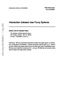
FIG. 1. Polymer density profiles ␾ p共r兲 surround two particles at the separation h = 20. The parameters are taken as N = 100, ␾0 = 0.1, ␹ = 0.5, and R = 10. The plot is obtained after transforming the bispherical coordinates to the Cartesian coordinates followed by a interpolation as to obtain an unform mesh.

tween two spheres are h = 20, 4 for Figs. 1 and 2, respectively. The radius of gyration of polymers is Rg ⯝ 4. At the surfaces of the two spheres the polymers density is zero, and it increases to the bulk concentration gradually far away from the spheres. From the figures we can easily find that the segments distribution varies greatly with the distance between the two spheres. When the distance is large, the density profiles near the two spheres are the same as in the depletion region near the surface of a single sphere. When the distance decreases to the polymer size, or when the depletion regions belonging to two spheres begin to overlap, the polymer segment concentration decreases rapidly. This decreasing is most distinct in the central region between two spheres. When the distance is smaller than some critical value 共depletion layer thickness兲, the density is quite low in the gap. The polymers go out of the gap for seeking more conformational entropy under the spatial confinement effect. However, in the plates case the critical value is about twice

FIG. 2. Polymer density profiles ␾ p共r兲 surround two particles at the separation h = 4. The parameters are taken as the same as those in Fig. 1 and the plot is transformed from the bispherical coordinates as that in Fig. 1.

FIG. 3. The maximum polymer concentration ␾max along the line of the centers of two spheres for ␹ = 0 and 0.5 as a function of separation h at different bulk concentrations. The parameters are taken as N = 100, ␾0 = 0.1, and R = 10.

of the thickness of depletion layer. We can conclude that the confinement effect is weaker than that in plates case and the polymers have more space to move. Even when the distance h is small, there are still a few segments in the gap between the two spheres 关10兴. It shows that the curvature effect is an important factor for depletion effect. Thus, the shape of the colloidal particles strongly affects the properties of a polymer-colloid dispersion 关2兴. In the gap between two spheres, there is a maximum value of polymer density along the line of centers of two spheres. The maximum values of ␾max as a function of the separation h at ␹ = 0 and ␹ = 0.5 are given in Fig. 3. As two spheres approach, the ideal polymers 共␹ = 0.5兲 without excluded volume effect are excluded from the gap prior to the polymers with excluded volume effect 共␹ = 0兲. The reason is that the depletion layer thickness in the ideal polymer solution is larger than that in the good solvent case.

B. Depleted amount and depletion potential

As the depletion layers belonging to two spheres become to overlap, the depletion effect occurs. It is necessary to investigate how the depleted amount and the depletion potential vary with the separation between two spheres. Figures 4 and 5 show the depletion potential and the depleted amount as a function of the separation h, respectively, in lower bulk concentration case or, ␾0 = 0.004− 0.04, which is in dilute regime. In this situation the polymer chains are isolated coils. The trends of the depletion potential are similar to those between two plates, in which the depth increases with increasing polymer concentrations. The range of potential remains nearly constant, which is about the order of the natural polymer size. We also found that the depleted amount relates to the depletion potential by U共h兲 / kBT = 关⌫共⬁兲 − ⌫共h兲兴 / N, which is the same as the result of Tuinier et al. for the dilute polymer solution 关18,20兴. This relationship can be obtained from the expression of Eq. 共9兲. When ␾ p共r兲 is much smaller than 1, using the relation ln共1 − ␾ p兲 ⯝ −␾ p − ␾2p / 2 we can obtain

041808-5


YANG et al.

FIG. 4. The depletion potential between two spheres as a function of the separation h in dilute solutions with ␾0 = 0.004, 0.01, 0.02, and 0.04. The parameters are taken as ␹ = 0.5, N = 100, and R = 10.

⌬F共h兲 =

冕冉冊 dr ␹ −

1 关共␾0兲2 − ␾2p共r兲兴 + 2

冕冋 dr

册

␾ − q共r,N兲 . N 共25兲 0

␹ = 0.5, and hence ⌬F共h兲 In ⌰ solvent end 0 ⯝ 兰dr关␾0 / N − ␾end 共r兲兴 ⯝ 兰dr关 ␾ − ␾ 共r兲兴 / N. Here, ␾ p p p 共r兲 represents the concentration of the end points of chains and we use the approximation ␾end p 共r兲 ⬇ ␾ p共r兲 / N. Thus, Eq. 共9兲 is reduced to U共h兲 / kBT ⬇ 关⌫共⬁兲 − ⌫共h兲兴 / N. An interesting result can be obtained by numerical fitting the depletion potential. The depletion potentials satisfy an universal function U共h兲 / 共kBT␾0兲 = −c1 exp共−hc2 / c3兲, where c1, c2, and c3 are constants depending on the parameters R, N, and ␹. For the current case the values are c1 = 13, c2 = 1.33, and c3 = 6, respectively. Figures 6 and 7 show the depletion potential and the depleted amount as a function of the separation h, respectively, in higher bulk concentration case or, ␾0 = 0.06− 0.2. The other parameters are the same as those in Figs. 4 and 5. In this case, the coils begin to overlap. The results are in qualitative agreement with those obtained by previous theoretical

FIG. 5. The depleted amount as a function of the separation h in dilute solutions with ␾0 = 0.004, 0.01, 0.02, and 0.04. The parameters are taken as the same as those in Fig. 4.

FIG. 6. The depletion potential between two spheres as a function of the separation h in semidilute solutions with ␾0 = 0.06, 0.1, and 0.2. The parameters are taken as the same as those in Fig. 4.

studies 关19兴 and experimental data 关29兴. The range of the potential decreases with increasing polymer concentration. Since the depletion potential comes from the overlap of two depletion layer belonging to two spheres, and the thickness of depletion layer decreases with increasing polymer concentration 关20兴, the depletion potential has the same width as the thickness of depletion layer. Different from dilute case, there is no universal function form in semidilute case. More importantly the minus of depleted amount as a function of h exhibits a barrier in semidilute solution. This indicates that when the two spheres approach to each other and the depletion layers of two spheres begin to overlap, the total number of polymers in system first decreases to the minimum, and then goes up 关see Eq. 共10兲兴. The height of barrier increases with increasing polymer concentration. In dilute solution the total number of polymers in the system always increases with decreasing h. This discrepancy indicates qualitatively different depletion effect in dilute and semidilute regime. Although the free energy of interaction between two objects is determined largely by the depleted amount of polymer 关10兴, the depletion potential between two spheres in the semidilute solution does not exhibit the barrier as the depleted amount. Thus, in the present study no repulsive force appears even when the bulk concentration is high, and the depletion interaction is always attractive.

FIG. 7. The depleted amount as a function of the separation h in semidilute solution with ␾0 = 0.06, 0.1, and 0.2. The parameters are taken as the same as those in Fig. 4.

041808-6



FIG. 8. The contribution from different parts of the grand potential and the grand potential as a function of the distance between two spheres in dilute regime for ␾0 = 0.02. The parameters are taken as the same as those in Fig. 4.

In order to understand the phenomenon further, we show the different parts of grand potential 关in Eq. 共7兲兴 as a function of h in the dilute and semidilute solutions. Figure 8 is for the dilute solutions with ␾0 = 0.02. In this case the interaction energy between the polymers and the solvents, the conformational entropy of polymers and the entropy of solvents increase monotonously with decreasing h. The compositive effect of those interactions is a monotonous attractive potential. In semidilute case, as shown in Fig. 9, the entropy of polymers increases monotonously. However, the interaction part first decreases and then increases as two spheres approach. It exhibits the minimum when h is about the thickness of depletion layer. The same behavior happens to the entropy of solvent. The compositive effect of those interactions is a monotonous attractive potential once again. This phenomenon shows that, although the depleted amount exhibits a barrier in semidilute regime, the solvents also play an important role, which adjusts the grand potential in such a way that the depletion potential remains attractive. The present continuous SCF model does not predict a repulsive depletion potential. However, in the lattice model adopted by Fleer et al. 关10兴 there exists an energy barrier when two plates approach at high polymer concentration. One possible

FIG. 9. The contribution from different parts of the grand potential and the grand potential as a function of the distance between two spheres in semidilute regime for ␾0 = 0.1. The parameters are taken as the same as those in Fig. 4.

FIG. 10. The contact depletion potential as a function of the bulk concentrations. The parameters are taken as the same as those in Fig. 4.

reason of the discrepancy is because of the different boundary conditions used in the different models. In the present model we impose the polymer density equal to zero at the surfaces of sphere. However, in the lattice model the segment concentration at the first layer near the surface is a nonzero value. The contact potential cannot be calculated because bispherical coordinates system does not exist for h = 0. However, we can extrapolate the curve of depletion potential to h = 0 is by numerical fitting. The extrapolated results is rather accurate since we can calculate the potential for very small h. Figure 10 displays the contact potential as a function of polymer concentration. It shows that U共0兲 is a linear function of ␾0. Eisenriegler has derived an exact result for the contact potential for the limit of low polymer concentration and large radius 关30兴 U共0兲 = − 4␲ ln 2

R2g 0 R␾ . N

The numerical prefactor in this equation is 2␲ / 3 ln 2 = 1.45. We find that our result is quite close to this result. This good agreement indicates that the above equation is also suitable to the situation with moderate size ratio of particle and polymer in semidilute ⌰ solution. Figure 11 shows the effect of solvency for ␹ = 0, 0.2, 0.4, and 0.5, respectively. The poorer the solvent is, the broader the range of the depletion potential is. The reason is that the thickness of depletion layer in the good solvent is thinner than that in the poor solvent. However, the contact potential is nearly the same for different solvency. The effect of polymerization N is presented in Fig. 12. The depth and the range of depletion potential increase as the chain length increases at a fixed bulk concentration. The experiment on the effect of molecular weight of nonadsorbing polymer on depletion-induced flocculation sustains the above results 关31兴. C. Consequences for colloidal stability

Once the quantitative depletion potential is obtained, we can investigate the colloidal stability induced by the deple-

041808-7


YANG et al.

FIG. 11. The effect of solvency on the depletion potential between two spheres as a function of separation h. The parameters are N = 100, R = 10, and ␾0 = 0.1.

tion interaction by calculating the second osmotic virial coefficient B2 defined as B2 = 2␲

冕

⬁

r2关1 − e−W共r兲兴dr,

FIG. 13. The second osmotic virial coefficient of hard spheres B*2 = B2 / 共4␲R3 / 3兲 as a function of the bulk concentrations ␾0 with the depletion potential calculated from SCFT and AO model, respectively. The parameters are taken as the same as those in Fig. 4.

␴PHS = 4Rg / 冑␲. The depletion potential between two spheres is

0

UAO共r兲 = − ␾0

where r = h + 2R is the center-to-center distance between two colloidal particles; W共r兲 is the total interaction potential between two particles. For hard spheres with only depletion interaction W共r兲 is given by W共r兲 =

再

⬁,

r ⬍ 2R,

U共r − 2R兲, r 艌 2R.

冎

The minus depletion potential will reduce B2. B2 is sensitive to the range and the strength of the depletion potential and it is a suitable measurement for the depletion effect when the colloid concentration is low enough and the many-body interactions can be ignored. If the depletion attractive interaction is strong enough, which can be achieved by increasing the polymer concentration and chain length, or decreasing solvency, B2 becomes sufficiently negative and the colloidal particles become unstable, and the phase separation or the flocculation will occur. As a reference, we calculate the Asakura and Oosawa 共AO兲 depletion interaction derived by Vrij 关12,18兴, the diameter of penetrable hard spheres is

+

冉冉

2 R + R g 冑␲

冊冋冉冊册 3

1 r 16 R + ␴PHS/2

1−

3 r 4 R + ␴PHS/2

冊

3

.

共26兲

Figure 13 gives the results for B*2 = B2 / 共4␲R3 / 3兲 as a function of polymer concentration using the depletion potential calculated by the SCFT and the AO model. The overlap concentration is about 0.1. From Fig. 13, we can conclude that when the spheres are the same order of the natural size of polymers and the polymer concentration is higher than the overlap concentration, B2 becomes negative enough. The value of B2 predicted by the AO model is much larger than ours. This means that in the AO model the depletion effect is underestimated seriously when the colloid suspensions and the polymers have the similar sizes. The underestimate becomes even worse with increasing polymer concentration. The result indicates that, in general, if the polymer size is comparable with the colloid particle size, the depletion induced phase separation in semidilute solutions is more profound than the previous theories predicted. V. CONCLUSION

FIG. 12. The effect of chain length on the depletion potential between two spheres as a function of separation h. The parameters are ␹ = 0.5, R = 10, and ␾0 = 0.1.

In this paper, the SCFT is employed to study the depletion interaction between two colloidal particles in nonadsorbing polymer solutions. The SCF equations are solved numerically in the bispherical coordinates to obtain the density profile in the space and the depletion potential. With increasing the separation between two spheres the polymers are pushed outside of the gap between two spheres due to spatial confinement. The results show that, in the dilute and semidilute solutions, the depletion interaction is always attractive, and no repulsive interaction appears. The present model does not predict the restability of the depletion effect in the semidilute regime. On the other hand, the depleted amount exhibits a barrier as a function of the separation between two spheres.

041808-8



The range of depletion potential is about the order of characteristic length of polymer solutions, and decreases with increasing polymer concentration in the semidilute solutions. The depth of the interaction increases with the increasing bulk concentration. The contact potential is proportional to bulk concentration in ⌰ solvent, even in the semidilute regime. The poor solvent has broader range for the depletion interaction. The longer the chain is, the stronger the attractive interaction is. Also, the stability of colloidal particles induced by depletion interaction has been investigated. High polymer concentration may induce the colloidal suspension to be unstable. Moreover, our results show that in the AO model the depletion effect was underestimated seriously when colloidal particles and polymers have similar sizes.

␾0p = ␾0 = Ne−␻pN ,

ACKNOWLEDGMENTS

0

共A2兲 0

␾s0 = 1 − ␾0 = e⌬␮se−␻s . Given the composite ␾0 we can obtain

␻s0,

and ⌬␮s by

1 ␾0 ln , N N

共A4兲

1 ␾0 ln − ␹共1 − 2␾0兲, N N

共A5兲

␻0p = −

␻s0 = −

共A3兲

␻0p,

⌬␮s = ln共1 − ␾0兲 −

1 ␾0 ln − ␹共1 − 2␾0兲. N N

共A6兲

The grand potential per unit volume is given by

We thank Professor Z. G. Wang for the stimulating suggestion on this subject. We also thank Professor R. A. Wickham and Dr. Weihua Li for the helpful discussions. This work is supported by National Natural Science Foundation of China 共NSFC兲 Grant Nos. 20340420327, 20474074, 20490220, 20575085, 20504027, and the 973 Project No. 2004CB720606. A.-C.S acknowledges support from the Natural Science and Engineering Research Council 共NSERC兲 of Canada.

g0 =

冉冊

1 ␾0 ␾0 G0 − = ␹共1 − ␾0兲2 + ln − 共1 − ␾0兲. V N N N 共A7兲

With the above results in homogenous state the different parts of excess free energy ⌬Fe, ⌬F p, and ⌬Fs are given by ⌬Fe =

冕

dr关␹␾ p共r兲␾s共r兲 − ␹␾0共1 − ␾0兲兴,

共A8兲

V

APPENDIX

⌬F p =

The SCF equations can be solved for a homogenous state with a bulk concentration ␾0. For such a case the density profiles ␾ p and ␾s, the propagator q and the self-consistent fields ␻ p and ␻s are constants and denoted with superscript 0. The solution of the modified diffusion equation is q0共t兲 = exp共−␻0pt兲. If we choose the exchange chemical potential of polymer ⌬␮ p = 0, the SCF equations are

␻0p − ␻s0 = ␹共1 − 2␾0兲,

dr ␻ p共r兲␾ p共r兲 − q共r,N兲 −

V

冉冊册

␾0 ␾0 ␾0 + , ln N N N 共A9兲

⌬Fs =

冕冋

dr ␻ p共r兲␾ p共r兲 − ␾s共r兲 −

V

共A1兲

关1兴 D. H. Napper, Polymeric Stabilization of Colloidal Dispersions 共Academic Press, New York 1983兲. 关2兴 R. Tuinier, J. Rieger, and C. G. de Kruif, Adv. Colloid Interface Sci. 103, 1 共2003兲. 关3兴 W. C. K. Poon, J. Phys.: Condens. Matter 14, R859 共2002兲. 关4兴 Y. Snir and R. D. Kamien, Science 307, 1067 共2005兲. 关5兴 S. Asakura and F. Oosawa, J. Chem. Phys. 22, 1255 共1954兲. 关6兴 P. G. de Gennes, Scaling Concepts in Polymer Physics 共Cornel1 University Press, Ithaca, NY, 1979兲. 关7兴 G. J. Fleer, M. A. Cohen Stuart, J. M. H. J. Schjeutjens, T. Cosgrove, and B. Vincent, Polymers at Interface 共Chapman & Hall, London, 1993兲. 关8兴 J. F. Joanny, L. Leibler, and P. G. de Gennes, J. Polym. Sci., Polym. Phys. Ed. 17, 1073 共1979兲. 关9兴 R. I. Feigin and D. H. Napper, J. Colloid Interface Sci. 75, 525 共1980兲. 关10兴 J. H. M. H. Scheutjens and G. J. Fleer, Adv. Colloid Interface

冕冋

册

− ␹共1 − 2␾0兲共1 − ␾0兲 + 共1 − ␾0兲 .

关11兴关12兴关13兴关14兴关15兴关16兴关17兴关18兴关19兴关20兴关21兴

041808-9

冉冊

1 − ␾0 ␾0 ln N N

共A10兲

Sci. 16, 361 共1982兲. S. Asakura and F. Oosawa, J. Polym. Sci. 33, 183 共1958兲. A. Vrij, Pure Appl. Chem. 48, 471 共1976兲. B. V. Derjaguin, Kolloid-Z. 69, 155 共1934兲. P. G. de Gennes, C. R. Seances Acad. Sci., Ser. B 288, 359 共1979兲. M. Schmidt, J. Phys.: Condens. Matter 11, 10163 共1999兲. E. Eisenriegler, J. Chem. Phys. 113, 5091 共2000兲. M. Fuchs, and K. S. Schweizer, Phys. Rev. E 64, 021514 共2001兲. R. Tuinier, G. A. Vliegenthart, and H. N. W. Lekkerkerker, J. Chem. Phys. 113, 10768 共2000兲. A. A. Louis, P. G. Bolhuis, E. J. Meijer, and J. P. Hansen, J. Chem. Phys. 117, 1893 共2002兲. R. Tuinier and G. J. Fleer, Macromolecules 37, 8764 共2004兲. M. Surve, V. Pryamitsyn, and V. Ganesan, J. Chem. Phys. 122, 154901 共2005兲.


YANG et al. 关22兴 J. Scheutjens, G. J. Fleer, and M. A. Cohen Stuart, Colloids Surf. 21, 285 共1986兲. 关23兴 K. M. Hong and J. Noolandi, Macromolecules 14, 727 共1981兲. 关24兴 S. M. Wood and Z. G. Wang, J. Chem. Phys. 116, 2289 共2002兲. 关25兴 J. R. Roan and T. Kawakatsu, J. Chem. Phys. 116, 7283 共2002兲. 关26兴 P. M. Morse and H. Feshbach, Methods of Theorical Physics 共McGraw-Hill, New York, 1990兲.

关27兴 G. B. Cook, Phys. Rev. D 44, 2983 共1991兲. 关28兴 W. F. Ames, Numerical Methods for Partial Differential Equation 共Academic, Boston, 1992兲. 关29兴 R. Verma, J. C. Crocker, T. C. Lubensky, and A. G. Yodh, Phys. Rev. Lett. 81, 4004 共1998兲. 关30兴 E. Eisenriegler, Phys. Rev. E 55, 3116 共1997兲. 关31兴 S. Biggs, J. L. Burns, Y.-D. Yan, G. J. Jameson, and P. Jenkins, Langmuir 16, 9242 共2000兲.

041808-10