meta-data such as depth cues, 3D points, or object decom- position in .... tial occurrence distributions for each codebook entry. Those ..... We define the minimum.
Depth-From-Recognition: Inferring Meta-data by Cognitive Feedback Alexander Thomas
Vittorio Ferrari
Bastian Leibe
Tinne Tuytelaars
Luc Van Gool
KU Leuven (BE)
University of Oxford (UK)
ETH Z¨urich (CH)
KU Leuven (BE)
KU Leuven (BE)
Abstract Thanks to recent progress in category-level object recognition, we have now come to a point where these techniques have gained sufficient maturity and accuracy to succesfully feed back their output to other processes. This is what we refer to as cognitive feedback. In this paper, we study one particular form of cognitive feedback, where the ability to recognize objects of a given category is exploited to infer meta-data such as depth cues, 3D points, or object decomposition in images of previously unseen object instances. Our approach builds on the Implicit Shape Model of Leibe and Schiele, and extends it to transfer annotations from training images to test images. Experimental results validate the viability of our approach.
1. Introduction Even when presented with a single image, a human observer can deduce a wealth of information, including the overall 3D scene layout, material types, or ongoing actions. This ability is only in part achieved by exploiting low-level cues such as colors, shading patterns, textures, or occlusions. At least equally important is the inference coming from higher level interpretations, like object recognition. Even in the absence of correct low-level cues, one is still able to estimate depth, as illustrated by the example of Fig. 1. These observations are mirrored by neurophysiological findings, as ‘low-level’ areas of the brain do not only feed into the ‘high-level’ ones, but invariably the latter channel their output into the former. The resulting feedback loops over the semantic level are key for successful scene understanding, see e.g. Mumford’s Pattern Theory [12]. The brain seems keen to bring all levels, from basic perception up to cognition into unison. These are exciting times for computer vision in that, for the first time, we are capable of implementing such cognitive feedback. Indeed, our community has made important strides forward in the recognition of object and action classes lately. The first examples of cognitive feedback have in fact already been implemented [7, 4]. However, so far
Figure 1. Humans can infer depth in spite of failing low-level cues, thanks to cognitive-feedback in the brain. Recognizing the buildings and the scene as a whole injects information about 3D structure (e.g. how street scenes are spatially organized, and that buildings are parallelepipeda). In turn this enables, e.g. to infer the vertical edges of buildings although they do not appear in the image. Besides, we are also able to estimate the relative depths between buildings, from this single image.
they only coupled recognition and crude 3D scene information (the position of the groundplane). Here we set out to demonstrate the wider applicability of cognitive feedback, by inferring ‘meta-data’ such as 3D object shape, material characteristics, or the location and extent of object parts, based on object class recognition. Given a set of annotated training images of a particular object class, we transfer these annotations to new images containing previously unseen object instances of the same class. The result can then be used to tune and robustify the low-level feature extraction for a refined scene interpretation. Such loop closure is reminiscent of adaptive acuity effects found in psychophysics. Here we focus on the inference from high-level recognition to low-level cues. We present a mechanism to automatically transfer object-oriented annotations, made explicit in training images, to test images. This mechanism is fully integrated within the recognition system. In a way, this work is akin to the concept of image analogies introduced by Hertzmann et al. [3]. Given a training image, its filtered version and a test image, a new analogously filtered image is synthesized.
In contrast to our work, such transfer is between low-level cues, replacing pixel patterns by filtered versions. In our setting, the differences between training and test images are usually too large to allow for a similar approach. Moreover, their method is computationally quite demanding and would be difficult to extend to the amount of data necessary to train object class detectors. Similarly, Hoiem et al. [5] estimate the coarse geometric properties of a scene by learning appearance-based models of surfaces at various orientations. By doing so, they are able to obtain rough 3D geometric information from a single image. Also there is no cognitive information involved, but the method relies solely on the statistics of small image patches. In [16], Sudderth et al. also combine recognition with coarse 3D reconstruction in a single image, by learning depth distributions for a specific type of scene from a set of stereo training images. In the same line, Saxena et al. [15] are able to reconstruct coarse depth maps for an entire scene by means of a Markov Random Field. Han and Zhu [2] obtain quite detailed 3D models from a single image through graph representations, but their method is limited to specific classes. As mentioned earlier, in their more recent work [4], Hoiem et al. do exploit cognitive-level information. They employ cars and pedestrians detected by an object class recognition method to update estimates of simple geometric properties of the scene (position of the horizon line and location of the ground plane). These are in turn used to remove false-positive object detections (e.g. those far above the horizon line). Similar ideas can be found in the work of Leibe et al. [7], but then for stereo images in the context of 3D city modeling. In both cases, the cognitive loop is implemented at high-level, reasoning about objects as a whole, without feedback to lower level data as we do. In the context of object recognition, Hoiem et al. have recently extended their Layout Conditional Random Field framework to input a 3D model, in order to recognize cars from multiple viewpoints [6]. Although their paper shows results on recognition only, their method might potentially also be applied to get an estimate of the depth for the car. The main contribution of this paper consists in closing the loop by providing a mechanism to go back from high level interpretations to low-level image processing. Accurate feedback of high-level recognition information to lowlevel cues involves more than simply backprojecting a single generic annotation mask. Indeed, the within-class variability needs to be taken into account. Building on the Implicit Shape Model proposed by Leibe and Schiele [8], we collect pieces of annotation from different training images and merge them into a novel annotation mask that matches the underlying image data. The paper is organized as follows. First, we recapitulate the Implicit Shape Model of Leibe and Schiele [8]
Original Image
Interest Points
Matched Codebook Entries
Probabilistic Voting
Voting Space (continuous)
Segmentation
Refined Hypothesis (optional)
Backprojected Hypothesis
Backprojection of Maximum
Figure 2. The recognition procedure of the ISM system.
for simultaneous object recognition and segmentation (section 2). Then follows the main contribution of this paper, as we explain how we transfer meta-data from training images to a previously unseen image (section 3). We demonstrate the viability of our approach by transferring both depth information as well as object parts for cars (section 4). Section 5 concludes the paper.
2. Object Class Detection with an Implicit Shape Model In this section we briefly summarize the Implicit Shape Model (ISM) approach proposed by Leibe & Schiele [8], which we use as the object class detection technique underlying our approach (see also Fig. 2). Given a training set containing example images of several instances of a certain category (e.g. sideviews of cars) as well as their segmentations, the ISM approach builds a model that generalizes over within-class variability. The modeling stage constructs a codebook of local appearances, i.e. of local structures that appear repeatedly on the training instances. The codebook entries are obtained by clustering image features sampled at interest point locations. Instead of searching for exact correspondences between a novel test image and candidate model views, the ISM approach maps sampled image features onto this codebook representation. We refer to the features in an image that are mapped onto a codebook entry as occurrences of that codebook entry. The spatial intra-class variability is captured by modeling spatial occurrence distributions for each codebook entry. Those distributions are estimated by recording all locations a codebook entry is matched to on the training objects, relative to the annotated object centers. Together with each occurrence, the approach stores a local segmentation mask, which is later used for inferring top-down segmentations. ISM Recognition. The ISM recognition procedure is formulated as a probabilistic extension of the Hough transform [8]. Let e be a sampled image patch observed at location ℓ. The probability that it matches to codebook entry ci can be expressed as p(ci |e). Each matched codebook entry then casts votes for instances of the object category on at different locations and scales λ = (λx , λy , λs ) according to
its spatial occurrence distribution P (on , λ|ci , ℓ). Thus, the votes are weighted by P (on , λ|ci , ℓ)p(ci |e), and the total contribution of a patch to an object hypothesis (on , λ) is expressed by the following marginalization: X P (on , λ|ci , ℓ)p(ci |e) (1) p(on , λ|e, ℓ) = i
The votes are collected in a continuous 3D voting space (translation and scale), and maxima are found using Mean Shift Mode Estimation with a scale-adaptive uniform kernel K [8]: � � 1 XX λ − λj pˆ(on , λ) = (2) p(o , λ |e , ℓ )K n j k k h(λ)3 h(λ) j k
Each local maximum in this voting space yields an hypothesis that an object instance appears in the image at a certain location and scale. Top-Down Segmentation. For each hypothesis, the ISM approach then computes a probabilistic top-down segmentation in order to determine the hypothesis’s support in the image. This is achieved by backprojecting the contributing votes to the image and using the stored local segmentation masks to infer the per-pixel probabilities that the pixel contains figure or ground given the hypothesis [8]. More precisely, the probability for a pixel p to be figure is computed as a weighted average over the segmentation masks of the occurrences of the codebook entries to which all features containing p are matched. The weights correspond to the patches’ respective contributions to the hypothesis at location x. p(p = f igure|on , x) P
P
= p∈e i p(p = f igure|e, ci , on , λ)p(e, ci |on , λ) P P i )p(ci |e)p(e) (3) = p∈e i p(p = f igure|ci , on , λ) p(on ,λ|c p(on ,λ)
We underline here that a separate local segmentation mask is kept for every occurrence of each codebook entry. Different occurrences of the same codebook entry in a test image will thus contribute different segmentations, based on their relative location with respect to the hypothesized object center. In early versions of their work [8], Leibe and Schiele included another optional processing step, where the hypothesis is refined by a guided search for additional matches in the test image (see also Fig. 2). This can improve the quality of the segmentations, but at a rather high computational cost. The procedure involved uniform sampling, which became untractable once scale-invariance was introduced into the system. We therefore implemented a more efficient refinement algorithm as explained in section 3.3. MDL Verification. In a last processing stage, the computed segmentations are exploited to refine the object detection scores, by taking only figure pixels into account.
Figure 3. Transferring (discrete) meta-data. Top row: two training images and their respective annotations. Bottom row: a test image. The corner of the license plate matches with a codebook entry which has occurrences on similar locations in the training images. The annotation patches for those locations are combined and instantiated in the output annotation (bottom right).
Besides, this last stage also disambiguates overlapping hypotheses. This is done by a hypothesis verification stage based on Minimum Description Length (MDL), which searches for the combination of hypotheses that together best explain the image. For details, we again refer to [8, 9].
3. Transferring Meta-data The power of the ISM approach lies in its ability to recognize novel object instances as approximate jigsaw puzzles built out of pieces from different training instances. In this paper, we follow the same spirit to achieve the new functionality of transferring meta-data to new test images. Example meta-data is provided as annotations to the training images. Notice how segmentation masks can be considered as a special case of meta-data. Hence, we transfer meta-data with a mechanism inspired by that used above to segment objects in test images. The training metadata annotations are attached to the occurrences of codebook entries, and transferred to a test image along with each matched feature that contributed to the final hypothesis (Fig. 3). This strategy allows us to generate novel annotations tailored to the new test image, while explicitly accommodating for the intra-class variability. Unlike segmentations, which are always binary, metadata annotations can be either binary (e.g. for delineating a particular object part or material type), discrete (e.g. for identifying all object parts), real-valued (e.g. depth values, or surface reflectance characteristics), or even vector-valued (e.g. surface orientations). We first explain how to transfer discrete meta-data (section 3.1), and then extend the method to the real-valued or vector-valued case (section 3.2).
3.1. Transferring Discrete Meta-data In case of discrete meta-data, the goal is to assign to each pixel of the detected object a label a ∈ {aj }j=1:N . We
first compute the probability p(p = aj ) for each label aj separately. This is achieved in a way analogous to what is done in eq. (3) for p(p = f igure), but with some extensions necessary to adapt to the more general case of meta-data.
P
p∈N (e)
P
p(p = aj |on , x) = a(p)=ae (p)|e)p(e,ci |on ,λ) i p(p=aj |ci ,on ,λ)p(ˆ
(4)
This will be explained in detail next. One extension consists in transferring annotations also from image patches near the pixel p, and not only from those containing it. With the original version, it is often difficult to obtain full coverage of the object, especially when the number of training images is limited. This is an important feature, because producing the training annotations can be labour-intensive (e.g. for the depth estimates of the cars in section 4). Our notion of proximity is defined relative to the size of the image patch e, and parameterized by a scalefactor sN . More precisely, let an image patch e be defined by the coordinates of its center and its scale eλ , i.e. e = (ex , ey , eλ ). The neighbourhood N (e) of e is defined as N (e) = {p|p ∈ (ex , ey , sN · eλ )}
(5)
A potential disadvantage of the above procedure is that with p = (px , py ) outside the actual image patch, the transferred annotation gets less reliable. Indeed, the pixel may lie on an occluded image area, or small misalignment errors may get magnified. Moreover, some differences between the object instances shown in the training and test images that were not noticeable at the local scale can now affect the results. To compensate for these phenomena, we add a factor to eq. (4), which indicates how probable it is that the transferred annotation ae (p) still corresponds to the ‘true’ annotation a ˆ(p). This probability is modeled by a Gaussian, decaying smoothly with the distance from the center of the image patch e, and with variance related to the size of e by a scalefactor sG : p a ˆ(p) = ae (p) | e with
�
σ
(dx , dy )
1 √ exp(−(dx 2 + dy 2 )/(2σ 2 )) σ 2π = sG · e λ
=
= (px − λx , py − λy )
(6)
Once we have computed the probabilities p(p = aj ) for all possible labels {aj }j=1:N , we come to the actual assignment: we select the most likely label for each pixel. Note how for some applications, it might be better to keep the whole probability distribution {p(p = aj )}j=1:N rather than a hard assignment, e.g. when feeding back the information as prior probabilities to low-level image processing. An interesting possible extension to the above scheme is to enforce spatial continuity between labels of neighboring pixels. This could be achieved either by smoothing, by
relaxation, or by representing the image pixels as a MRF. However, whether this is applicable depends on the actual semantic meaning of the annotations, and on the application scenario. In the two scenarios we experimented with (inferring object part labels, and 3D depth values), we achieved good results already without enforcing spatial continuity. The practical implementation of this algorithm requires rescaling and resampling the annotation patches. In the original ISM system, bilinear interpolation is used for rescaling operations, which is justified because segmentation data can be treated as probability values. However, interpolating discrete labels such as ’windshield’ or ’bumper’ does not make sense. Therefore, rescaling must be carried out without interpolation.
3.2. Transferring Real- or Vector-valued Meta-data In many cases, the meta-data is not discrete, but rather real-valued or vector-valued. For example 3D depth is realvalued, and surface orientation is vector-valued. Ideally, we should extend the method from the previous paragraph to work with real-valued data in all phases of the process. However, we can also approximate the real-valued case by using a large number of quantization steps. This has the advantage that we can re-use most of the same system as for the discrete case. Additionally, it avoids problems inherent with some types of real-valued data, for instance continuity constraints. The following approach, which produces continuous annotations by passing through a discrete approximation first, delivers good results (section 4.1). First, we discretize the annotations into a fixed set of ‘value labels’ (e.g. ‘depth 1’, ‘depth 2’, etc.). This allows to proceed in a way analogous to eq. (4) to infer for each pixel a probability for each discrete value. In the second step, we select for each pixel the discrete value label with the highest probability, as before. Next, we refine the estimated annotation value by fitting a parabola to the probability scores for the maximum value label and the two immediate neighbouring value labels, and selecting the value corresponding to the maximum of the parabola. This is a similar method as used in interest point detectors ([1, 10]) to determine continuous scale coordinates and orientations from discrete values. Thanks to this interpolation procedure, we obtain real-valued annotations. In our 3D depth estimation experiments this makes a significant difference in the quality of the results (section 4). In the case of vector valued meta-data, the same procedure can be followed, only now with a (D + 1)-dimensional paraboloid.
3.3. Refining Hypotheses When large areas of the object are insufficiently covered by interest points, no meta-data can be assigned to these areas. Using a large value for sN will only partly solve
this problem, because there is a limit as to how far information from neighboring points can be reliably extrapolated. A better solution is to actively search for additional codebook matches in these areas. The refinement procedure in early versions of the ISM system [8] achieved this by means of uniform sampling, which is untractable in the scale-invariant case. Therefore we implemented a more efficient refinement algorithm which only searches for matches in the most promising locations. For each initial hypothesis, new candidate points are generated by backprojecting all occurrences in the codebook, according to the location and scale of the hypothesis. Points nearby existing interest points are omitted. When the feature descriptor for a new point matches with the codebook cluster(s) that backprojected it, an additional vote is cast for the hypothesis. The confidence for this new vote can be reduced by a penalty factor to reflect the fact that it was not generated by an actual interest point. The additional votes enable the meta-data transfer to cover those areas that were initially missed by the interest point detector. This refinement step can either be performed on the final hypotheses that result from the MDL verification, or on all hypotheses that result from the initial voting. In the latter case, it will improve MDL verification by enabling it to obtain better figure area estimates of each hypothesis [8, 9]. This makes the refinement procedure part of a small cognitive loop within the recognition system.
4. Experimental evaluation We evaluate our approach on two different scenarios for the object class car. In the first, we recover a 3D depth map, indicating for each pixel the distance from the camera (a real-valued labeling problem). We stress that this is achieved from a single image of a previously unseen car. In the second scenario, we aim at decomposing the car in its most important parts (wheels, windshield, etc.), which is a discrete labeling problem. Our dataset is a subset of that used in [7]. It was obtained from the LabelMe website [14], by extracting images labeled as ‘car’ and sorting them according to their pose. For our experiments, we only use the ‘az300deg’ pose, which is a semi-profile view. In this pose both the front (windscreen, headlights, license plate) and side (wheels, windows) are visible. This allows for more interesting depth maps and part annotations compared to pure frontal or side views. The dataset contains a total of 139 images. We randomly chose 79 for training, and 60 for testing.
4.1. Inferring Depth Information In our first experiment, the idea is to infer approximate 3D information from recognized cars. A possible scenario is an automated car wash. Even though most automated
Figure 4. Obtaining depth maps for the car images. Left shows the original image, middle the image with the most suitable 3D model superimposed (notice how the model for the second car is a completely different brand, but still fits fairly well). The rightmost images show the depth maps obtained from the 3D model.
car wash systems are equipped with sensors to measure the distance to the car, they are only used locally while the machine is already running. It could be useful to optimize the washing process beforehand, based on the global shape of the car. Training We trained an ISM system on the 79 training images, using a Hessian-Laplace interest point detector and Shape Context descriptors. These have been shown to yield superior performance in previous evaluations [11]. In our cognitive-feedback approach, we input a depth map as meta-data for each training image. In general, any applicable method like structure-from-motion or a laser scanner could be used to automatically obtain depth maps. In order to reuse an existing dataset for which training depth maps are not available, we used a custom approach which consists in manually aligning a 3D car model on top of each image. The depth map is then derived from the aligned 3D models. This method produces maps which are more accurate and smooth than when using SFM, which could be hampered by the specularities on typical cars. We collected a set of 223 3D models from the website “DMI car 3D models”1 , and converted them to a standard format (VRML97). A custom OpenGL application was written to align the models with the images. It allows to superimpose the 3D model over the image semitransparantly, and manipulate its pose and camera parameters until it matches sufficiently. An accurate depth map can easily be obtained by extracting the OpenGL Z-buffer (Fig. 4). Unfortunately, the 3D models are not designed to match the ordinary cars present in the LabelMe images. Most 1 http://dmi.chez-alice.fr/models1.html
3D models cover high-range, but unfortunately uncommon, cars such as the Bugatti Veyron. Nevertheless, for nearly all training images we could pick a 3D model with a shape similar to the car in the image. For a few exceptional images, we assembled a custom 3D model by combining parts from other 3D models. A second problem is ensuring that the depth maps are consistent with each other, which is required for our method to produce correct annotations on new test images. We normalize the depth maps, based on the fact that cars have approximately the same width w. We define the minimum and maximum depth for each 3D model as dmin = zc − r, dmax = zc + r respectively, with zc the Z-coordinate of the model’s center. The radius r is calculated as the model’s actual width, multiplied by a factor 1.75. This ensures no part of the 3D model lies outside the allowed depth range, in any pose. By rescaling all depth values within a range from 0 for dmin to 1 for dmax , the depth maps are effectively normalized. An approximate real-world depth (relative to the car’s center, which has depth 0.5) can be estimated from the normalized values by multiplication by 3.5w. We quantize the normalized depth maps to 20 discrete values and use our method of section 3.2 to transfer the depth maps. Testing The recognition part of this experiment is only moderately challenging because each image contains exactly one car at a similar scale as the training data. However, our goal is not to demonstrate the recognition performance of ISM (which was thoroughly investigated in previous works [8, 9]). Instead, we want to evaluate depth map annotations generated by our extension to the system (section 3.2). Hence we run the standard recognition procedure of section 2 on each image, and select the detection with highest score for meta-data transfer. The refinement procedure of section 3.3 was performed on all initial hypotheses. A few of the resulting depth maps are shown in Fig. 5. The results look good, especially considering the limitations of our training data. Note how the depth maps adapt to the actual shape of the car, which would be impossible when fitting a generic car model to the detection. To evaluate the experiment quantitatively, we calculate a set of scores based on statistics gathered over all images. We define leakage as the percentage of background pixels in the ground-truth annotation that were labeled as nonbackground by the system. The leakage for this experiment, averaged over all test images, is 4.79%. We also define a coverage measure, as the percentage of non-background pixels in the ground-truth image labeled non-background by the system. The coverage obtained by our algorithm is 94.6%. This means our method is able to reliably segment the car from the background. To evaluate the error in depth reconstruction, we con-
Figure 5. Results for the depth map experiment. The left column shows the test images, the middle column ground truth depth maps, and the right column the output of our system. The light blue areas are unlabeled and can be considered background.
sider the average absolute value of depth differences. Because the background is the largest area in all images and its depth value is arbitrary, it would be unfair to calculate the average error over the entire image. The system’s figure-background separation ability is already captured in the coverage and leakage measures. Therefore we only consider the pixels that are labeled ‘object’ in both the training and test images. The average error measure over this area is 0.042. To convert this error to a real-world value, we measured the average width w of a car (side mirrors included) to be approximately 1.8m. Multiplying the depth error by 3.5w yields an approximate real-world distance, as explained in the ‘Training’ paragraph, of 0.27m. The resulting depth maps are of course not absolute, but relative to the object’s centers. In an application where an
Figure 6. Example training object decompositions.
absolute depth is required, the distance from the camera to the object should be estimated, e.g. based on the scale of the detection and camera parameters, or obtained from a system like [15], and added to the relative depth values.
4.2. Object Decomposition Another scenario where cognitive feedback is desirable, is traffic surveillance. A traffic control system may automatically detect and attempt to identify each individual car, in order to track it across multiple, active cameras. The first stage in this process is the detection of each car. Next, some kind of unique identifier, such as the license plate, is required. To facilitate the reading of the license plate on an unknown image of an arbitrary car, it would be useful to know where to look in the image. Humans know immediately where the plate is located, because they recognize the car. Actually, the license plate itself might even have contributed to the recognition. In contrast, classic computer vision approaches typically search the whole image. This is slow and unreliable. Due to its small scale and uncharacteristic shape, many image areas look like license plates, resulting in many false-positive detections. In this experiment, we use a different type of meta-data on the same dataset. It illustrates how the recognition of the car can go hand-in-hand with identifying its subparts (among which, the license plate). In our system, the license plate provides cues for recognizing the car (local image patches fed into the ISM), and in turn recognizing the car gives very strong information about the location of the license plate (through meta-data transfer). Training The ISM system was trained as in the previous experiment, this time with discrete meta-data. We annotated each car image by labeling the following parts: chassis (body), bumpers, headlights, wheels, license plate, and windows (including windshield). The rest of the image is labeled ‘background’. Only visible parts are annotated. Occluded parts and parts that can’t be discerned from the shadow, are labeled ‘background’. Figure 6 shows a few
Figure 7. Results for the object parts annotation experiment. The left column shows the test images, the middle column the groundtruth annotations, and the right column the output of our system. The light grey areas are unlabeled and considered background. Note how the system successfully detects the lack of a license plate for the fourth car.
example annotations. The segmentations required for training the ISM system are obtained by mapping all car part labels to ‘foreground’. Testing The same type of test as for the previous experiment is run, but this time we apply the discrete method from section 3.1, with the annotation maps as meta-data. Examples of resulting annotations are shown in Fig. 7. We evaluate the annotations quantitatively by a confusion matrix between the ground-truth annotations and those produced by the system. For each image, we count how many pixels of each part aj are labeled as each of the possible parts (body, bumpers, etc.), or remain unlabeled (which
bkgnd body bumpr headl windw wheel licen
bkgnd 23.56 4.47 7.20 1.51 3.15 11.38 2.57
body 2.49 72.15 4.54 36.90 13.55 6.85 1.07
bumpr 1.03 4.64 73.76 23.54 0.00 8.51 39.07
headl 0.14 1.81 1.57 34.75 0.00 0.00 0.00
windw 1.25 8.78 0.00 0.01 80.47 0.00 0.00
wheel 1.88 1.86 7.85 0.65 0.00 63.59 1.04
licen 0.04 0.24 2.43 0.23 0.00 0.01 56.25
unlab 69.61 6.05 2.64 2.41 2.82 9.65 0.00
Table 1. Confusion matrix for the object parts annotation experiment. The rows represent the annotation parts in the ground-truth maps, while the columns represent the output of our system. The last column shows how much of each class was left unlabeled by our algorithm (light grey in the images). For most evaluations, unlabeled areas can be considered equivalent to ‘background’.
among which a further verification of the detection itself. The latter would close the cognitive loop for the recognition system. Future research includes both investigating such cognitive loops, and further improving the performance of the meta-data transfer. Next, we will implement support for fully real-valued meta-data. Finally, we will explore using our system output as a shape prior to drive shape-fromshading approaches, such as [13]. Acknowledgements The authors gratefully acknowledge support by IWT-Flanders, Fund for Scientific Research Flanders and European Project CLASS (3E060206).
References can be considered background in most cases). This score is normalized by the total number of pixels in the ground-truth a ˆj . We average the confusion table entries over all images, resulting in table 1. The diagonal elements in the table show how well each part was recovered in the test images. The system performs well as it labels correctly between 56% and 80% of pixels (except for the headlights), depending on the part. We consider this a very encouraging result, especially considering the high challenge presented by the task, owing to intraclass variability, remaining viewpoint and scale changes, specular reflections, and the diverse material nature and size of parts to be labeled. As expected, confusion is highest between parts covering a small area (e.g. headlights, license plate) and the larger parts in which they are embedded (body, bumper, respectively). We can also calculate the leakage and coverage as in the previous experiment. The leakage is 6.83% and coverage is 95.2%. To get an idea of the overall quality of labeling itself, we can calculate the percentage of mislabeled pixels. However, similarly to the depth map experiment, it would be unfair to include the background due to its large area. Therefore we only consider pixels that are both labeled non-background in the reference annotation and the system’s output. This yields an average error of 20.8%.
5. Conclusions We have developed a method to transfer meta-data annotations from training images to test images, based on a highlevel interpretation of the scene. Instead of using an independent (post-)processing step for inferring the meta-data, it is deeply intertwined with the actual recognition process. Low-level cues in an image can lead to the detection of an object (in our experiments, cars), and the detection of the object itself causes a better understanding of the low-level cues from which it originated. The resulting meta-data inferred from the recognition can be used in several ways,
[1] H. Bay, T. Tuytelaars, and L. V. Gool. Surf: Speeded up robust features. Proceedings ECCV, Springer LNCS, 3951(1):404–417, 2006. [2] F. Han and S.-C. Zhu. Bayesian reconstruction of 3D shapes and scenes from a single image. Workshop Higher-Level Knowledge in 3D Modeling Motion Analysis, 2003. [3] A. Hertzmann, C. Jacobs, N. Oliver, B. Curless, and D. Salesin. Image analogies. SIGGRAPH, 2001. [4] D. Hoiem, A. Efros, and M. Hebert. Putting objects in perspective. CVPR, pages 2137–2144, 2006. [5] D. Hoiem, A. A. Efros, and M. Hebert. Geometric context from a single image. ICCV, 2005. [6] D. Hoiem, C. Rother, and J. Winn. 3D LayoutCRF for multiview object class recognition and segmentation. CVPR, 2007. [7] B. Leibe, N. Cornelis, K. Cornelis, and L. V. Gool. Integrating recognition and reconstruction for cognitive traffic scene analysis from a moving vehicle. DAGM, pages 192– 201, 2006. [8] B. Leibe and B. Schiele. Interleaved object categorization and segmentation. BMVC, 2003. [9] B. Leibe and B. Schiele. Pedestrian detection in crowded scenes. CVPR, 2005. [10] D. G. Lowe. Distinctive image features from scale-invariant keypoints. IJCV, 60(2):91–110, 2004. [11] K. Mikolajczyk and C. Schmid. A performance evaluation of local descriptors. PAMI, 27(10), 2005. [12] D. Mumford. Neuronal architectures for pattern-theoretic problems. Large-Scale Neuronal Theories of the Brain, pages 125–152, 1994. [13] M. Prasad, A. Zisserman, and A. Fitzgibbon. Single view reconstruction of curved surfaces. CVPR, 2006. [14] B. Russell, A. Torralba, K. Murphy, and W. Freeman. LabelMe: a database and web-based tool for image annotation. MIT AI Lab Memo AIM-2005-025, 2005. [15] A. Saxena, J. Schulte, and A. Y. Ng. Learning depth from single monocular images. NIPS 18, 2005. [16] E. Sudderth, A. Torralba, W. Freeman, and A. Willsky. Depth from familiar objects: A hierarchical model for 3d scenes. CVPR, 2006.