Available online at www.sciencedirect.com
ScienceDirect Energy Procedia 75 (2015) 1856 – 1861
The 7th International Conference on Applied Energy – ICAE2015
Derivation and Comparison of Open-loop and Closed-loop Neural Network Battery State-of-Charge Estimators Ala A. Hussein* *
Electrical Engineering Department, United Arab Emiates University, Al Ain, United Arab Emirates, P.O. Box: 15551
Abstract This paper presents two artificial neural network (ANN) based algorithms for battery state-of-charge (SOC) estimation. The SOC is an important quantity that must be estimated in real-time in many applications. ANN is a mathematical model that consists of interconnected artificial neurons inspired by biological neural networks and is used to predict the output of a dynamic system based on some historical data of that system. The first algorithm presented in this paper has an open-loop structure and known as nonlinear input output (NIO) feed-forward algorithm, while the second is closed loop called nonlinear autoregressive with exogenous input (NARX) feed-back algorithm. A pulse-discharge test is performed on a commercial lithium-ion (Li-ion) battery cell in order to collect data to evaluate those methods. Results are presented and compared. © Published by Elsevier Ltd. This © 2015 2015The TheAuthors. Authors. Published by Elsevier Ltd.is an open access article under the CC BY-NC-ND license (http://creativecommons.org/licenses/by-nc-nd/4.0/). Selection and/or peer-review under responsibility of ICAE Peer-review under responsibility of Applied Energy Innovation Institute
Keywords: Artificial neural network (ANN); battery; state-of-charge (SOC).
1. Introduction
Li-ion batteries must be carefully charged and discharged in order to prolong their cycle-life and ensure a safe operation. Overcharging these batteries produces excessive heat that could damage the battery, shorten its lifetime, and further, result in a fire hazard, where over-discharging batteries could result in an irreversible damage or reduced service-time [1], [2]. In order to have a reliable battery operation without exceeding the battery’s design limits, the amount of the input/output energy must be accurately determined. To achieve that, an accurate battery SOC estimator must be implemented in the battery management system. Similar to the concept of a fuel gauge, an SOC estimator must provide an accurate value of the amount of energy in the battery as a percentage of its total capacity [3]. Unlike a fuel gauge, the SOC is an immeasurable quantity that is rather estimated. Nonetheless, there are several methods that can be used to estimate the SOC ranging from simple to sophisticated methods. Those methods can be classified into two types: direct and indirect. Some examples of direct methods include current-integration or “coulomb
* Corresponding author. Tel.:+971-3-713-5332. E-mail address:
[email protected].
1876-6102 © 2015 The Authors. Published by Elsevier Ltd. This is an open access article under the CC BY-NC-ND license (http://creativecommons.org/licenses/by-nc-nd/4.0/). Peer-review under responsibility of Applied Energy Innovation Institute doi:10.1016/j.egypro.2015.07.163
1857
Ala A. Hussein / Energy Procedia 75 (2015) 1856 – 1861
counting”, which is one of the most common methods used to estimate the SOC. Although currentintegration method can be implemented in real-time and can be very accurate, it has one major limitation due to its open-loop nature. That is, with a very small error in the current measurement, the estimated SOC can easily diverge from the true SOC value after few cycles due to accumulated error in the current measurement unless a reset mechanism is periodically used [4], [5]. Another direct method that is used to estimate the SOC is the “open-circuit voltage”. In this method, the voltage is measured continuously and the corresponding SOC is obtained from a lookup table. This method requires a very low (dis)charge current for accurate results, which can be a good choice for some applications that draw very small currents from the battery. Other methods such as the “discharge test” is not practical because it wastes the energy stored in the battery and cannot be used in real-time. In addition, the “impedance spectroscopy” method requires an AC current injection into the cell to measure its impedance and is hard (if not impossible) to achieve dynamically [6], [7]. On the other hand, there are several indirect methods that are used to estimate the SOC. Those methods can be very accurate and reliable in general. Among those methods is artificial neural network (ANN). ANN methods don’t rely on any electrical, physical, chemical, or thermal model and they have superior characteristics such as high robustness and accuracy. However, ANN methods require huge data to train the network in order to calculate the weight functions for the network [4], [8], [9]-[16]. The paper presents and compares common ANN models for SOC estimation including an open-loop and closed-loop models. The organization of this paper is as follows: Section 2 presents some experimental test results obtained from a commercial Li-ion battery cell. In Section 3, ANN-based SOC estimators are derived. Section 4 is a summary of the presented models. Finally, conclusion is drawn in Section 5. 2. Battery Data
In order to compare the presented methods, some battery cell data were gathered from a commercial 1.1Ah, 3.6V Li-ion cell. A pulse-discharge test was performed over the entire capacity range of the cell. In this test, the true SOC value is obtained by integrating the current with time (coulomb-counting). The battery was fully charged using constant current/constant voltage profile, then it was discharged using a 1A pulse current. Since the test comprises only one cycle, the SOC calculated using coulomb-counting is believed to be 100% accurate and thus it will be used later as a reference. The voltage and SOC are shown in Figure 1. 3.6
1
0.8
0.6 SOC
Voltage (V)
3.4
3.2
0.4 3
2.8
0.2
0
10
20
30
40 50 Time (min)
(a)
60
70
80
90
0
0
10
20
30
40 50 Time (min)
(b)
60
70
80
90
Figure 1. (a) Cell’s voltage during pulse discharge test (left), and (b) the cell’s SOC.
3. Artificial Neural Networks (ANN)
ANN is a mathematical tool that is inspired by the way the human brain processes information [8]. ANNs consist of a number of layers each of which consists of a number of processing units called
1858
Ala A. Hussein / Energy Procedia 75 (2015) 1856 – 1861
“neurons” as the basic unit. The neurons are interconnected through weight functions as shown in Figure 2(a). Figure 2 (b) shows a diagram of an adaptive ANNs operation.
(a) (b) Figure 2. (a) A two-layer feed-forward ANN with 10 hidden neurons, n input neurons and 1 output neuron, and (b) an operational block diagram of an ANN (right).
ANNs are highly stable and robust due to their massive parallel structure. ANNs consist of inputs and outputs and are made of neurons interconnected with each other. The weights in Figure 2 are determined during the training phase and their values determine how the neural network will respond to a particular series of inputs. Thus, training ANNs is the most critical phase that determines how accurate those ANNs are. The weights of an ANN are calculated in the training phase by minimizing the loss function (usually a quadratic function of the output error). One common technique that is widely used in training ANNs is the back-propagation, or back-propagation of errors, which is a supervised learning method that is commonly used in the training phase to calculate the weights of a neural network. Back-propagation uses a steepestdescent technique based on the computation of the gradient of the loss function with respect to the network parameters, [17]. To evaluate the performance of ANNs in estimating the SOC, two common network architectures were selected: the first is nonlinear input-output (NIO) feed-forward network, and the second is nonlinear autoregressive with exogenous input (NARX) feed-back network. For both networks, LevenbergMarquardt back-propagation algorithm was used in training. 3.1 NIO Feed-forward Network This network predicts one time series given the current and past values of an input time series as shown in Figure 4. For the purpose of estimating the SOC, the input time series x(t) consists of the battery terminal voltage and current, where the output or target is the SOC. The output equation of this network is given in (1).
y (t ) = f ( x (t − 1), ..., x (t − d ))
(1)
3.2 NARX Feed-back Network This network predicts one time series given the current and past values of an input time series as well as the past and current values of another time series, called external or exogenous time series (output). A block diagram of this network is shown on Figure 5. The output equation of this network is given in (2).
y (t ) = f ( x (t − 1), ..., x(t − d ), y2 (t − 1), ..., y (t − d ))
(2)
In (1) and (2): f(.) represents the unknown function in Figure 3, x(t) indicates the input time series that consists of the cell’s terminal voltage and current, y(t) is the output time series which is the actual SOC, and d is a delay parameter (d = 1, 2, 3, …). For both networks, the delay parameter indicates the delay in the input/output time series and it can be selected by trial and error until the desired accuracy is obtained.
1859
Ala A. Hussein / Energy Procedia 75 (2015) 1856 – 1861
The number of neurons in the hidden layer was set at 10. The value of the delay parameter and the number of neurons in the hidden layer were purposefully varied in order to find the effect of the selected values on the network performance. The results of estimating the SOC for both the NIO and NARX models are shown in Figures 3. The value of the delay parameter d was values of 2, 4, 6, 8 and 10. NIO (d=2)
NARX (d=2)
1
1
0.5
0.5
0
0
20
40
60
80
0
100
0
20
NIO (d=4) 1
0.5
0.5 0
20
40
60
80
0
100
0
20
NIO (d=6)
40
60
80
100
80
100
80
100
80
100
0.5 0
0
20
40
60
80
100
0
20
NIO (d=8) 1
0.5
0.5 0
20
40
40
60
NARX (d=8)
1
60
80
100
0
0
20
NIO (d=10)
40
60
NARX (d=10)
1
1
0.5
0.5
0
100
1 SOC
SOC
1
0
80
NARX (d=6)
0.5 0
60
NARX (d=4)
1
0
40
0 0
20
40 60 Time (min) True SOC
80
Estimated SOC
(a)
100
0
20
40 60 Time (min) True SOC
Estimated SOC
(b)
Fig. 3. Results of estimating the SOC with delay values 2, 4, 6, 8, and 10 using NIO (a) and NARX (b) feed-forward ANNs.
4. Comparative Summary of Results
The results in Figure 3 are obtained after the process and measurement were contaminated by adding a zero-mean process noise with an absolute peak value of 10mA and a zero-mean measurement noise with an absolute peak value of 10mV to the current and voltage readings. The reason for adding these noises is to run the tests under practical circumstances. Both the process and measurement noises are independent and Gaussian. Obviously in Fig. 3, NARX networks obviously outperformed NIO networks due to their feedback loop. In the presented NARX models, the feedback loop was used in the training phase to calculate the weight functions. The feedback resulted in a more accurate performance as can be seen by comparing the NARX and NIO models. However, although the calculated weight functions for both the NIO and NARX models are optimal in the sense that they gave the best possible performance, the weight functions must be able to adapt to changes in the ambient conditions or battery parameters.
1860
Ala A. Hussein / Energy Procedia 75 (2015) 1856 – 1861
It was shown that as the delay parameter d increases in the NIO network, the noise in the estimated SOC decreases, while for the NARX network, there was no noise in all cases, which is another advantage of the feed-back loop. Also, it was found that there is no correlation between the network accuracy and the number of neurons in the hidden layer. It was noticed that when the number of neurons in the hidden layer is less than 5, the accuracy is slightly lower than when the number of neurons is above 5. However, the performance of the network didn’t change at all when the number of neurons in the hidden layer was changed randomly between 5 and 100 for both NIO and NARX networks. 5. Conclusion
In this paper, two ANN-based models for battery SOC estimation were derived and compared. The results show that the two models can perform well if they were trained with an artificial experience similar to the real experience. To practically implement the presented ANN SOC estimators, advanced hardware (i.e. sensors, memory, microprocessor, etc.) must be used, which will consequently lead to a relatively high implementation cost. Practically, ANN estimators can be used in applications where the current is very dynamic such as in electric vehicles. In low- or steady- current applications such as portable electronics, however, simple methods like coulomb-counting and open-circuit voltage are considered satisfactory and can be implemented at a relatively low cost. Acknowledgements This research was supported in part by the United Arab Emirates University under startup research grant # G00001287.
References [1] [2] [3] [4] [5] [6] [7] [8] [9] [10] [11] [12] [13] [14]
R. C. Cope and Y. Podrazhansky “The art of battery charging” The Fourteenth Annual IEEE Battery Conference on Applications and Advances, 1999. A. A. Hussein and I. Batarseh “A review of charging algorithms for nickel and lithium battery chargers” IEEE Transactions on Vehicular Technology, vol. 60, no. 3, pp. 830-838, 2011. A. A. Hussein and I. Batarseh “State-of-charge estimation for a single Lithium battery cell using Extended Kalman Filter” IEEE Power and Energy Society General Meeting, 2011. A. A. Hussein “Capacity Fade Estimation in Electric Vehicles Li-ion Batteries using Artificial Neural Networks”, 2013 ECCE Conference, Denver, Colorado, 2013. G. L. Plett “Extended Kalman filtering for battery management systems of LiPB-based HEV battery packs: Part 3. State and parameter estimation”, Journal of Power sources, vol. 134, no. 2, pp. 277-292, 2004. S. Piller, M. Perrin and A. Jossen “Methods for state-of-charge determination and their applications, Journal of power sources, 96.1 (2001): 113-120. A. A. Hussein, N. Kutkut, J. Shen and I. Batarseh “Distributed Battery Micro-Storage Systems Design and Operation in a Deregulated Electricity Market”, IEEE Transactions on Sustainable Energy, vol. 3, no. 3, pp. 545-556, 2012. S. Haykin “Neural Networks and Learning Machines”, pp. 1-46, 3rd edition, pp. 1-46, 1999. C.C. Chan, E.W.C. Lo and S. Weixiang, “The available capacity computation model based on artificial neural network for lead– acid batteries in electric vehicles” Journal of Power Sources, vol. 87, no. 1-2, pp. 201-204, 2000. P. Shi, C. Bu and Y. Zhao “The ANN Models for SOC/BRC Estimation of Li-ion Battery” IEEE International Conference on information Acquisition, 2005. W. X. Shen, C. C. Chan, E. W. C. Lo and K. T. Chau “A new battery available capacity indicator for electric vehicles using neural network”, Energy Conversion and Management, vol. 43, no. 6, pp. 817-826, 2002. T. Yamazaki, K. Sakurai and K. Muramoto “Estimation of the residual capacity of sealed lead-acid batteries by neural network”, INTELEC conference, pp. 210-214, 1998. A. Affanni, A. Bellini, C. Concari and G. Franceschini “EV battery state of charge: neural network based estimation”, IEEE International Electric Machines and Drives Conference, 2003. W. X. Shen “State of available capacity estimation for lead-acid batteries in electric vehicles using neural network”, Energy Conversion and Management, vol. 48, no. 2, pp. 433-442, 2007.
Ala A. Hussein / Energy Procedia 75 (2015) 1856 – 1861
[15] W. X. Shen, K. T. Chau, C. C. Chan and E. W. C. Lo, “Neural network-based residual capacity indicator for nickel-metal hydride batteries in electric vehicles”, IEEE Transactions on Vehicular Technology, pp. 1705 – 1712, 2005. [16] C. H. Cai, D. Du, Z. Y. Liu and H. Zhang “Artificial neural network in estimation of battery state of-charge (SOC) with nonconventional input variables selected by correlation analysis”, International Conference on Machine Learning and Cybernetics Proceedings, 2002. [17] H. S. Hippert, C. E. Pedreira and R. C. Souza "Neural networks for short-term load forecasting: A review and evaluation." IEEE Transactions on Power Systems, vol. 16, no. 1, pp. 44-55, 2001.
1861