Derivation of a curve number and kinematic-wave

Hydrologîcal Sciences-Journal-des Sciences Hydrologiques, 46(4) August 2001

571

Derivation of a curve number and kinematic-wave based flood frequency distribution R. S. KUROTHE Central Soil and Water Conservation Research and Training Institute, Research Centre, Vasad District, Anand, Gujarat 388 306, India

N. K. GOEL & B. S. MATHUR Department of Hydrology, University ofRoorkee, Roorkee 247 667, India e-mail: goelnfhvfairurkiu.ernetin Abstract The physically-based flood frequency models use readily available rainfall data and catchment characteristics to derive the flood frequency distribution. In the present study, a new physically-based flood frequency distribution has been developed. This model uses bivariate exponential distribution for rainfall intensity and duration, and the Soil Conservation Service-Curve Number (SCS-CN) method for deriving the probability density function (pdf) of effective rainfall. The effective rainfall-runoff model is based on kinematic-wave theory. The results of application of this derived model to three Indian basins indicate that the model is a useful alternative for estimating flood flow quantiles at ungauged sites. Key words curve number; kinematic wave; flood frequency; physically-based distribution; regionalization

Une distribution fréquentielle des crues déduite de courbes numérotées et de l'onde cinématique Résumé Les modèles à bases physiques de fréquence de crue s'appuient sur des données de pluie et des caractéristiques du bassin versant facilement disponibles pour déduire la distribution de la fréquence des crues. Nous présentons dans cette étude une nouvelle distribution des fréquences de crue à bases physiques. Ce modèle utilise une distribution exponentielle bivariée de l'intensité et de la durée de la pluie, et la méthode des courbes numérotées ("curve number") du Soil Conservation Service (SCS) américain, pour estimer la fonction de densité de probabilité (fdp) de la pluie nette. Le modèle pluie nette-débit est basé sur la théorie de l'onde cinématique. Les résultats de l'application de ce modèle à trois bassins versants indiens montrent que ce modèle est une alternative pertinente pour estimer les quantiles de débits de sites non jaugés. Mots clefs courbes numérotées; onde cinématique; fréquence de crue; distribution à bases physiques; régionalisation

INTRODUCTION Very few methods exist for the estimation of the probability density function (pdf) of flood discharges for catchments without discharge measurements. These methods include (a) transfer of streamflow records from a nearby river basin of a hydrometeorologically homogeneous region using a drainage area scaling relationship; (b) use of flood frequency methods such as index flood or regional regression methods (see e.g. Stedinger et al., 1993; Cunnane, 1988). Each of these has attendant problems (e.g. Burn & Goel, 2000; Goel et al., 2000). Physically-based, derived flood frequency distribution (DFFD) models offer a promising alternative to traditional regional flood frequency methods. Open for discussion until 1 February 2002

572

R. S. Kurothe et al,

The DFFD models were first introduced by Eagleson (1972). These models are analytical combinations of the following three major components: (a) a stochastic rainfall model, (b) an infiltration model, and (c) an effective rainfall-runoff model. Since their inception, researchers have tried different models for the above listed major components. Based on the effective rainfall-runoff model used, the available DFFD models may be broadly categorized as (a) kinematic-wave (KW) theory based DFFD models and (b) geomorphological instantaneous unit hydrograph (GIUH) and geomorphoclimatic IUH (GcIUH) based DFFD models. A brief review of available DFFD models follows. Kinetic-wave theory based DFFD models Eagleson (1972) used bivariate exponential distribution of rainfall intensity and duration in combination with a constant loss rate ( | index) infiltration model. A kinematic-wave runoff model was used for transformation of effective rainfall distribution into distribution of peak discharge. Shen et al. (1990) used the Philip infiltration equation (Diaz-Granados et ah, 1984) for derivation of the pdf of effective rainfall. The effective rainfall-runoff model used by Eagleson (1972) was modified to include five different regimes of flow. Cadavid et al. (1991) applied the stochastic rainfall and infiltration models used by Shen et al. (1990) and also included one of the regimes omitted by Eagleson (1972) in their effective rainfall-runoff model. Kurothe (1995) applied various KW theory based DFFD models for different combinations of component models to various catchments ranging from 42.7 to 178 km2 located in central India. The pdf of the effective rainfall intensity and the duration was derived using the 0

(1)

where (3 and 8 are the inverses of mean areal storm intensity and mean storm duration, respectively. Intensity and duration are assumed independent of each other. This approximation may not be satisfactory in situations where a significant correlation exists between these variables. For such situations, the models developed by Kurothe et al. (1997) and Goel et al (2000) might be more appropriate. Probability distribution function of effective rainfall intensity and duration The curve number method (SCS, 1985, 1993) computes the excess rainfall depth, R, as a function of the total rainfall depth, P, and the maximum potential retention, S (a function of curve number CN). Excess rainfall depth is given by:

o2

R = (P(P-I a+S)

P>Ia

(2a)

R == 0

Pt0

(4)

Derivation of a curve number and kinematic-wave based flood frequency distribution

575

and te

for tr < t()

*e

(5)

Also, 0.25 t„ =

.

0.2S

(6)

or i =

Storms with intensities of 0

The continuous part of the joint pdf of ie and te can be expressed as the product of equations (9) and (10): f

a \

f

ieje (h > O = 0.77642p8exp(-8? e - a)T(a + 1)(T0

v'A; /

\ 0.44161

ie, te > 0

(11)

•exp -1.39047p \hj

Effective rainfall-runoff model The basin is conceptualized as two symmetrical planes discharging into a first-order stream. The relationship of peak discharge with rainfall parameters and catchment parameters is obtained by using kinematic-wave theory. For the details of kinematicwave theory and its solution by the method of characteristics, see Eagleson (1970). Eagleson (1972) considered three cases for peak discharge calculations. Cadavid et al.

R. S. Kurothe et al.

576

(1991) presented the relationships between peak discharge, Qp, and rainfall and catchment parameters for four cases. Flood frequency distribution The cdf of peak discharge, Qp, is obtained by integration of the joint pdf of ie and te over regions where Qp is less than or equal to a given value. These regions are shown in Fig. 1. Using the relationship between Qp as a function of ie, te and other catchment characteristics and the boundaries of the integration region (Cadavid et al., 1991), the cdf of Qp is computed as: ¥Qp{Qp)^PNR+fj\f,e,re(ie,te)àieàte

(12)

'=1 R,

The return period, T, for a given value of Qp is given by (Eagleson, 1972; DiazGranados et ah, 1983): 1 T =(13) ffiv[l-F0(e„)] where mv is the average number of independent rainfall events per year. The derivation °f Fg (QP ) is presented in Appendix A. MODEL APPLICATION RESULTS The curve number and KW theory based DFFD model has been applied to three basins in Central India, namely Tairhia, Pausar, and Kharanala. The basins have different size, shape and land uses; all three basins have clayey soil (Table 2). t,

t, + t„ t , = t,

Fig. 1 Integration regions for computations of cdf of peak discharge.

Derivation of a curve number and kinematic-wave basedfloodfrequency distribution

577

Table 2 Details of basins and rainfall model parameters. Description Longitude (E) Latitude (N) Length of annual peak discharge data (years) Area (km2) Soils Land use* Curve number P (h cm'1) S(lh 4 ) mv Time of concentration (h) *C: cultivated; F: forest; B: barren.

Tairhia 79°50'08" 22°52'36" 20

Pausar 78°21'56" 22°45'25" 24

Kharanala 77°02'20" 20°59'25" 22

101.0 Clay with gravels: 96% Rocks: 4% C: 9.6% F: 86.5% B: 3.9% 83 6.33 0.075 62.3 6

67.37 Clay: 100%

42.7 Clay: 100%

C: 60% F: 40%

C: 100%

85 4.687 0.124 69.5 4

91 7.852 0.113 63.7 3

Parameters of component models For the basins under study, hourly rainfall and annual flood series were obtained from original registers (RDSO, 1991) and were processed before application of the developed model. The computation of the parameters of the component models is described below. Stochastic rainfall model parameters There are three parameters to be estimated using rainfall data: the number of independent events per year, mv, the inverse of mean areal rainfall intensity, P, and the inverse of mean storm duration, 8. The parameters P and S are used to represent the joint distribution of areal rainfall intensity and duration. The parameter mv is used for computing the return periods of various peak discharges. The rate of arrival, i.e. number of storms per unit time (mv if the unit time is equal to one year) depends upon how the storms are separated from each other. In the present study, the two storms were considered to be independent of each other if the interevent time was greater than the time of concentration. The time of concentration for these basins was computed assuming that water moves through a basin as sheet flow, shallow concentrated flow and open channel flow before reaching the outlet (SCS, 1985). The storms so separated were then used to compute mean intensity and mean duration of different storms of the basins. The values of p, 8 and mv so obtained for the three watersheds are given in Table 2. Curve number Soil and land use data were used to estimate the curve numbers for each of the basins. Curve numbers were assigned from the standard tables published by SCS (1985, 1993) for each combination of soil type and land use and weighted average curve numbers were then calculated for each basin. The percentage area covered by different soils and


578

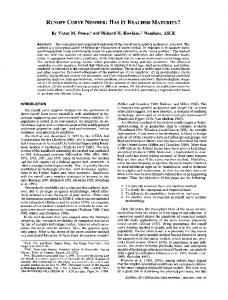
land uses in the catchment and the weighted average curve numbers for the basins under study are given in Table 2. Kinematic-wave parameters The KW effective rainfall-runoff model requires following parameters: - length of the main channel, Lc - width of the overland plane, W - channel slope, sc - overland plane slope, sp - Manning's roughness coefficient for channel, nc - Manning's roughness coefficient for plane, np and - coefficient a and exponent b of the hydraulic radius-area relationship. The main channel length of each watershed was measured using a planimeter. The basin area was divided by twice the length of the main channel to obtain the average plane width. The plane slope was computed using the grid method and the equivalent channel slope was computed by Gray's method (Singh, 1993). Channel roughness coefficients were assigned based on the general characteristics of the channel. The estimation of the roughness coefficient for a plane is slightly difficult, but recent studies in catchment hydrology make it possible to estimate this even for ungauged catchments (see e.g. Gaur, 1999). Gaur (1999) has represented the temporal variation of overland plane roughness with the size and slope of a basin. However, in the present work, a constant value of 0.3, which was considered some sort of average value for the whole study area (subzone 3 c) was adopted. The values of a and b were taken as 0.175 and 0.35, respectively. The kinematicwave parameters for these basins are listed in Table 3. The discharge vs return period (Q-T) relationships The discharge vs return period (Q-T) relationships were developed using equation (13) for the three watersheds. The Q-T relationships are shown in Figs 2-A for Tairhia, Pausar and Kharanala basins, respectively. This model is being designated as curve number-kinematic-wave derived flood frequency distribution (CN-KW-DFFD) model. The observed annual maximum discharge data have also been plotted in these figures along with 95% confidence intervals. The confidence intervals were constructed by fitting a lognormal distribution to the flood discharge observations at each site and estimating 95% confidence limits about a true distribution. Table 3 Kinematic-wave parameters for the test basins. Parameter Length of stream Width of plane Slope of the channel Slope of the plane Manning's roughness coefficient for channel

Symbol Lc W

Units (m) (m)

Sc

sP nc

-

Tairhia 32893.5 1335.26 0.004304 0.072267

Pausar 24046.0 1400.86 0.00243 0.030432

Kharanala 23567.0 907.74 0.002937 0.005614

-

0.040

0.023

0.021


579

1400

—*- Observed CDF

1200

- • - 9 5 % Jpper confidence limit

jt

95% _ower confidence limit -,

CN4CW-DFFD

*

^'

/ ' P l o t Area [

/

E

U

/

onal

/

800

c

/ /

600

y

-

" " ^

7s*

s*

*>*

^M.

^ ^'

y 400

/

rZ

200

mWf

100 Return Period (years)

Fig. 2 Comparison of DFFD model with 95% confidence intervals associated with observed flood discharges for the Tairhia basin.

It may be seen from Figs 5-7 that the cdfs of the CN-KW-DFFD model lie well within the 95% confidence intervals. Although the DFFD model is not always able to reproduce the observed cdf of flood discharges, these are enclosed by 95% confidence intervals for the most part, especially in the upper tail of the distribution. In order to judge the relative performance of the developed model, the Q-T relationships were also developed by regional flood frequency analysis (RFFA). Regional flood frequency analysis was carried out using standardized probability weighted moments (Hosking et ah, 1985) for Extreme Value Type I (EV-1) distribution. For subzone 3C, utilizing the annual peak discharge data at 10 bridge sites having catchment areas ranging from 53.68 to 2110.85 km2, the following relationships were developed: Qm=\l.\2-A

0.6056

r = 0.812

(14)

and or/gave = u + oc{-ln[-ln(l - 1/T)]} [/= 0.7013, a = 0.5175

(15) where Qave is the mean annual flood (m s" ), A is catchment area (km ), ris the coefficient of correlation, T is the return period (years), QT is the T years return period flood quantile, and u and a are the regional location and scale parameters of the EV-1 distribution. The same curves are also shown in Figs 5-7 for comparison. 3

1

2


580

Return period [years]

Fig. 3 Comparison of DFFD model with 95% confidence intervals associated with observed flood discharges for the Pausar basin.

The relative performance of the models was judged on the basis of the absolute value of relative error in the top most (i.e. first) and top six flood quantiles (when arranged in decending order), respectively, as follows: ABSERRT

^AbS(Qiobs-Qiam)

(16)

and ABSERRT6 = j A b s ( a , b s -fi c o m p )/6

(17)

where ABSERRT is the absolute relative error in the top most quantile, and ABSERRT6 is the average absolute relative error in the top six quantiles; Qi0bs is the rth observed quantile, and QiCOmp is the ith computed quantile. The ABSERRT and ABSERRT6 indices give the comparison in the upper tail region of the frequency curve. The values of the above indices are presented in Table 4 for both the CN-KW-DFFD model and RFFA. For the Tairhia and Pausar basins, the modified DFFD model performs better than the RFFA. In the case of Kharanala basin, the RFFA estimates are quite close to the observed cdf. The performance of the DFFD model is not as good as that of RFFA, however, The cdf of the DFFD model also falls within the 95% confidence intervals. The results, in general, can be termed quite reasonable considering the data requirement of the model developed in the study.

Derivation of a curve number and kinematic-wave basedfloodfrequency distribution

581

1200

f

1000

1 1 / 4

•

m

i Upper confidence limit 95>Î Lower confidence limit CM KW-DFFD

/

600

— » - O b i served CDF

~-*-Rec

/

/ 400

?

"

»

200

& 10

100

Return Period (years)

Fig. 4 Comparison of DFFD model with 95% confidence intervals associated with observed flood discharges for the Kharanala basin.

Table 4 Comparative performance of DFFD model with regional analysis (Q,„ = highest flood). Performance criterion

CN-KW-DFFD model: ABSERRT ABSERRT6 3 1 = 606 m s ) 25 Tairhia basin (Qm 150 74 Pausar basin {Qm = 4 1 0 n r V ) 155 Kharanala basin (Q„, = 390 itf s"1) 159

Regional analysis (RFFA) : ABSERRT ABSERRT6 106 96 51 169 38 22

CONCLUSIONS A physically-based flood frequency distribution has been derived using joint pdf of exponentially distributed rainfall intensity and duration, curve number for excess rainfall computation and kinematic wave as effective rainfall-runoff model. The use of the curve number method is simple and the data required for estimation of curve numbers are readily available. This provides an alternative approach for flood frequency determination and produces quite reasonable results. However, this model needs to be applied to additional catchments for which long-term rainfall and runoff data are available. Application of the model with regionalized values of rainfall parameters may greatly simplify the flood frequency estimation for ungauged basins.

582


REFERENCES Burn, D. H. & Goel, N. K. (2000) The formation of groups for regional flood frequency analysis. Hydrol. Sci. J. 45(1), 97-112. Cadavid, L., Obeysekara, J. T. B. & Shen, H. W. (1991) Flood-frequency derivation from kinematic wave. J. Hvdraul. Engng ASCE 117(4), 489-510. Cordova, J. R. & Rodriguez-lturbe, I. (1985) On the probabilistic structure of surface runoff. Wat. Resonr. Res. 21(5), 755-763. Cunnane, C. (1988) Methods and merits of regional flood frequency analysis. J. Hydrol. 100(1/3), 269-290. Diaz-Granados, M. A., Valdes, J. B. & Bras, R. L. (1983) A derived flood frequency distribution based on the geomorphoclimatic IUH and density function of rainfall excess. Report no. 292, Massachusetts Inst, of Tech., Cambridge, Massachusetts, USA. Diaz-Granados, M. A., Valdes, J. B. & Bras, R. L. (1984) A physically based flood frequency distribution. Wat. Resour. Res. 20(7), 995-1002. Eagleson, P. S. (1970) Dynamic Hydrology. McGraw-Hill, New York, USA. Eagleson, P. S. (1972) Dynamics of flood frequency. Wat. Resour. Res. 8(4), 878-898. Gaur, M. L. (1999) Modeling of surface runoff from natural watersheds with varied roughness. Unpublished PhD Thesis, Department of Hydrology, University of Roorkee, Roorkee, India. Goel, N. K., Kurothe, R. S., Mathur, B. S. & Vogel, R. M. (2000) A derived flood frequency distribution for correlated rainfall intensity and duration. J. Hydrol. 228, 56-67. Hebson, C. & Wood, E. F. (1982) A derived flood frequency distribution using Horton order ratios. Wat. Resour. Res. 18(5), 1509-1518. Hosking, J. R. M., Wallis, J. R. & Wood, E. F. (1985) Estimation of the Generalised Extreme Value distribution by the method of probability weighted moments. Technometrics 27(3), 251-261. Kurothe, R. S. (1995) Development of physically based flood frequency models. Unpublished PhD Thesis, Department of Hydrology, University of Roorkee, Roorkee, India. Kurothe, R. S., Goel, N. K. & Mathur, B. S. (1997) Derived flood frequency distribution for negatively correlated rainfall intensity and duration. Wat. Resour. Res. 33, 2103-2107. Moughamian, M. S., McLaughlin, D. B. & Bras, R. L. (1987) Estimation of flood frequency: an evaluation of two derived distribution procedures. Wat. Resour. Res. 23(7), 1309-1319. Ponce, V. M. & Hawkins, R. M. (1996) Runoff curve number: has it reached maturity? J. Hydrol. Engng ASCE 1(1), 1 1 19. Raines, T. H. & Valdes, J. B. (1993) Estimation of flood frequencies of ungauged catchments. J. Hydraul. Engng ASCE 119(10), 1138-1154. RDSO (Research, Design and Standards Organization) (1991) Estimation of design discharge based on regional flood frequency approach for sub zones 3(a), 3(b), 3(c) and 3(e). Research, Design and Standards Organization, Lucknow, India. Rodriguez-lturbe, I. & Valdes, J. B. (1979) The géomorphologie structure of hydrologie response. Wat. Resour. Res. 15(6), 1409-1420. Rodriguez-lturbe, I. Gonzalez-Sanabria, M. & Bras, R. L. (1982) A geomorphoclimatic theory of instantaneous unit hydrograph. Wat. Resour. Res. 18(4), 877-886. SCS (Soil Conservation Service) (1985) National Engineering Handbook. Section 4, Hydrology. Soil Conservation Service, USDA, Washington, DC, USA. SCS (1993) National Engineering Handbook. Section 4, Hydrology, Chapter 4. Soil Conservation Service, USDA, Washington, DC, USA. SCS (1986) Urban hydrology for small watersheds. Technical Release no. 55 (TR-55), Soil Conservation Service, USDA, Washington, DC, USA. Shen, H. W., Koch, G. J. & Obeysekara, J. T. B. (1990) Physically based flood features and frequencies. J. Hydraul. Engng ASCE 116(4), 495-514. Singh, V. P. (1993) Elementary Hydrology. Prentice Hall of India (Pvt. Ltd.), New Delhi, India. Stedinger, J. R., Vogel, R. M. & Foufoula-Georgiou, E. (1993) Frequency analysis of extreme events. In: Handbook of Hydrology (ed. by D. R. Maidment). McGraw-Hill, New York, USA.


583

APPENDIX A Derivation of Fe (Q ) in equations (12) and (13) Integration of equation (11) in the direction of ie, between iei and z'e2, ie\ < Ui, yields: f'2f,

T

(ie,te)die = f20.77642pôexp(-5?e -o)r(o + l)a-°

yhK

(Al)

/ n^

• exp

-1.39047P

dr \*.J AoA

Substituting A = 0.77642p8 exp(-5?e - a)T(q + l ) o " \Kj / f'*2 i?

/•

, 1 * f*«2 . - 0 44161

, \i>

J fle,Te(h,te)àie=A

I ze

exp

\ 0.44161

-1.39047P

ai. /

Substituting

(A2)

Khj \0.44161

/V, = 0.44161, y = il~k' and 5*=1.39047p

and changing the

limits:

'el

'el

1

Jf/e,re Od*; = ^* J 7—^exp(-5>)dy (A3) = ,4

1-A, Substituting A and S in the above equation one obtains: f oA

J f,eJe (ie, te )die = S exp(-S/e - a)T(a + l)o "\ exp-1.39047p v?ey 0.44161

-exp -1.39047P

(A4)

= g(*'el>*'e2>0

Figure 1 shows the integration region for computation of the cdf of Qp. Cadavid et al. (1991) covered the integration region casewise (case 1 to case 4) by seven integrals. For simplicity, the itegration area is covered by four portions as shown in Fig. 1, This avoids the use of iterative methods to compute the conditions at the boundaries of different cases. The iterative method is used only for the solution of equations of peak

584


discharge for QP2 and QPA. Integrating equation (B4) with respect to te for the four portions with respective limits and adding PNR yields: F, (Qp) = Pm+F

g(h = 0,ie for QpUte)dte + tg(ie

= 0,ie for Qp2,te)dte

+ f ug(ie = 0,ie for Qp4,te)dte + Jf-43 g(ie = 0,ie for Qp3,te)dte

(A5)

The integrals in equation (B5) are computed numerically. The first integral having an upper limit of infinity is computed until a specific tolerance is attained. Received 1 August 2000; accepted 26 February 2001