Derivation of Response Time Service Level Objectives for Business Services David Breitgand, Ealan Henis, Onn Shehory
John M. Lake
IBM Research Lab Haifa, Israel Email: {davidbr,ealan,onn}@il.ibm.com
IBM Tivoli, Durham, NC, USA Email:
[email protected]
Abstract— Design of Service Level Agreements (SLAs) emerges as an increasingly important discipline in business-oriented IT management. In this work, we study utility maximization of contractual obligations of a business service provider for a typical SLA. We demonstrate that using service usage and performance data as well as IT performance data, routinely collected by enterprises, efficient automated derivation of optimal response time Service Level Objectives (SLOs) of an SLA is possible. This paper addresses a specific facet of the SLA design problem not sufficiently addressed in previous studies. One common approach is to calculate SLOs attainable for the given IT infrastructure by means of simple percentile analysis. However, this methodology is business agnostic and may result in sub-optimal SLOs. Another widespread approach addresses IT infrastructure (re)design, where the goal is to enable the IT to meet specified target SLOs. In contrast to these approaches, our work proposes finding optimal response time SLOs attainable for the given IT infrastructure in a business aware manner. We define the response time SLO optimization problem, propose an algorithm that efficiently solves it using linear optimization and percentile analysis, and evaluate our solution both analytically and experimentally.
I. I NTRODUCTION A Service Level Agreement (SLA) between a service provider and a service consumer formalizes non-functional requirements on the service provisioning. Commonly used non-functional requirements relate to performance, security, availability, business continuity, etc. These requirements are explicitly specified in Service Level Objectives clauses (SLOs) of an SLA. Typically, a penalty is incurred on the provider for non-compliance with the SLOs. In this work we focus on response time SLOs of the business services. A typical response time (RT) SLO clause defines the following: •
•
• • • •
Target average response times of service transactions at various load levels (alternatively – at different time windows during a typical business day; we also call them usage windows); Means for sampling average response time for verification of compliance with the target values; Sampling frequency; Compliance evaluation period; Penalty terms and conditions for non-compliance; Allowed percentage of breaches of the target average response times during the evaluation period. We call this quantity ”breach budget”.
The concept of breach budget is central in our work. Simply put, if the total number of average response time breaches is within the breach budget, no penalty is incurred on the service provider. Hence, the capability of service provisioning within the breach budget is highly desirable for a service provider. A simple percentile analysis is often used to identify a low risk breach budget for a given IT infrastructure [1]. However, even if the total number of breaches detected during an evaluation period is within the allowed budget, the SLO may be suboptimal from other business perspectives. Generally, the same transactions executed at different times during a business day may have different value for the service provider. This observation calls for optimization of breach budget distribution across usage windows, aiming at maximizing utility for the service provider. A breach budget distribution scheme is implemented by setting specific average response time target values for each usage window. Thus, the optimization problem boils down to deriving per-window response time target values, such that the total sum of business gains and losses is maximized. Manually solving such a problem is not scalable. To assist service and IT managers in solving this problem, we have developed an automated tool – Automated Derivation of response time Service Level Objectives (ADSLO). To illustrate the problem and our solution approach, consider a typical situation as depicted in Figure 1(a). An enterprise, e.g., an air carrier (shown at the bottom), provides a flight reservation service. A consumer of this service, the travel agency (at the top), consumes the service in the context of an SLA it signed with the air carrier. In the scenario depicted by Figure 1(a), the internal IT department of the air carrier supports provisioning of the flight reservation service. The question we answer in the context of this scenario using the ADSLO approach is: What are the optimal response time SLOs that the service provider (air carrier) can support without additional investment in its IT infrastructure, judging solely by the historical performance of the service (flight reservation), historical performance of IT infrastructure, and typical usage of the service? In this scenario, a Chief Information Officer (CIO) is required by her management to commit to a level of response time for the core business service without adding IT resources or starting costly and time consuming restructuring and fine tuning of existing IT. The problem that the CIO has to solve
II. P ROBLEM S TATEMENT We start with informal problem formulation. In Section IIB, we state the problem rigorously. A. Informal Problem Statement For the sake of simplicity, we first consider a single transaction of a single business service. In Section VIII we show how the simple solution can be extended in a straightforward manner to the more complex case of concurrent optimization of multiple SLAs and SLOs.
Uses
Business Service SLA terms
Flight Reservation
terms
Business Service SLA
terms
Travel Agency
terms
Travel Agency
Flight Reservation
Air Carrier
Air Carrier
IT Department
IT Department
a) ADSLO user is Carrier's CIO
Outsourced
Uses
is to identify attainable SLOs, which are aggressive enough to satisfy the management, while realistic enough to mitigate the risk of SLA breaching. The ADSLO tool provides the CIO with insights into the optimal attainable SLOs at a very low effort. Presenting the automatically derived optimal SLOs to business-level management will allow the latter to assess to which extent current attainable IT performance is aligned with the business needs of the enterprise. This is the core task of Business Service Management [2]. Management decisions resulting from this analysis may include capacity re-planning, IT tuning, or deciding to apply no changes, as the current IT performance meets business needs. The ADSLO approach is different from, and complementary to, an important line of research, exemplified in [3], [4]. That research addresses capacity planning and sizing given specific target SLOs. Our solution may be used to assess the need for capacity planning given a specific system, its historical performance, and business service historical usage patterns. In case that capacity re-planning is required, ADSLO provides hints regarding the current gap in service performance to be bridged by capacity enhancement or restructuring. Figure 1(b) represents a slightly different scenario. In this scenario, the IT of the carrier is out-sourced to an external IT provider. An IT provider needs to prepare an IT service offering its customer (in this case, the carrier). An SLA needs to be negotiated such that the customer is satisfied (aggressive response time SLOs while achieving business level objectives), yet only low risk of SLA breach is imposed on the provider. Again, the IT provider is interested in finding out which SLO levels it can commit to without additional investments in infrastructure. In this paper, we formally define the problem of response time SLO derivation as a linear optimization problem. We derive optimal response time target values for each identified usage window. Other parameters of a response time SLO, such as breach budget, are considered fixed and translate into a system of constraints. We build a model, which takes into account the financial impact of transactions meeting/missing their deadlines, as well as transactions usage trends and historical performance data. The model includes a utility function, which captures the transaction’s value for the service provider at different usage windows. We present our algorithm, describe a prototypical implementation, and perform an extensive experimental and analytical evaluation.
External Provier b) ADSLO user is external Provider
Fig. 1. Example scenarios: (a) IT provider is internal; (b) IT provider is external
Since usage of computing systems reflect human activities, the usage history of a service is not random. If one considers transaction usage (measured, say, by number of invocations) recorded during an SLA evaluation period, patterns corresponding to different time windows during the business day are easily identified. We term these windows usage windows. Figure 2 shows an shopping transaction usage pattern obtained from running a sample e-commerce application on our experimental system.1 Modern SLA monitoring and management tools such as ITSLA [5] allow an administrator to divide an SLA evaluation period into N usage windows (possibly of various sizes), where each window may have a different relative importance. For example, if most of the usage (e.g., 40%) occurs between 2PM to 5PM, this time window may be defined as ”critical usage window”. If between 1AM to 6AM there is almost no transaction activity, the window may be defined as ”off time window”, etc. We may expect the business (IT consumer) to define usage windows manually,2 or via some automatic process. Once the windows are defined, historical usage patterns for each window may be extracted from the historical usage data. In a business environment, each transaction incurs a financial impact on the business: a gain if the transaction succeeds and a loss if it fails. In the context of this work, we ignore multiple criteria for transaction failure/success, and focus exclusively on timeliness. Thus, a transaction fails if it misses its target deadline, and succeeds otherwise. We assume that the average per-transaction gain and loss values for different usage windows are known. These values are important inputs to an optimization process that attempts 1 The 2 This
experiments are discussed in detail in Section V. is a common practice in some management tools, e.g., ITSLA [5].
to maximize the total value for the service provider. If absolute values are not available, relative values would suffice. For example, relative values may be provided by stating that the transaction value during the prime window is twice that during the normal window.3
Number of Invocations of "AccountServlet"
180
Symbol N Wi RTi Pi si bi Ci C
160
Ci−
140 120
Ci+
100
Ai RTA-SLO
80
Definition Number of usage windows Usage window i Target response time for Wi Probability that a transaction breaches its RTi in Wi Value gained if a transaction meets RTi in Wi Loss incurred if a transaction breaches RTi Number of transaction executions in Wi Number of transaction executions during PN entire integration interval: C = C i=1 i Number of transaction executions, which breached RTi in Wi Number of transaction executions, which met RTi deadline in Wi Relative usage pertaining to Wi : Ai = CCi Response Time SLO. See Figure 3
60
U (P )
40 20 0
0
500
Fig. 2.
1000 Time (5 min resolution)
1500
2000
Utility function: U (P1 , ..., PN ) = PN PN A (1 − Pi )si − APb i=1 i i=1 i i i (see Section III for details) TABLE I N OTATION
Sample Transaction Usage Pattern
Suppose that a compliance evaluation period (also referred to as integration interval) of one week is specified for the SLA. Assume that a measurement for checking response time compliance is run every 5 minutes. 2016 measurements will be performed during the integration interval. Let P ortion denote the level of compliance as specified in the response time SLO clause. P ortion equal to, say, 0.97 means that 97% of the tests (1956) have to be successful (i.e., meet their target RT values). The fraction of allowed unsuccessful tests, the breach budget, is 1 − P ortion. If the breach budget is violated, the SLA is breached and the service provider should pay a penalty. Setting an RT target for each usage window will render some of the transaction executions as compliant with that target, while others will breach that RT target. To fully specify the response time SLO clause definition, the CIO should determine the target response times, which will correspond to the required P ortion with high probability. This problem is commonly solved using percentile analysis. Simply put, a cumulative distribution function Fn is computed for a historical response times sample of sufficiently large size n. Then Fn−1 (P ortion) yields the needed target response time. While this approach is simple and valid, one should notice that the resulting target response times are agnostic to business needs. Consequently, the SLA designed this way may be suboptimal in terms of total utility for the service provider. In each usage window the transaction success/failure may carry a different financial gain/loss for the business. Our optimization goal is to maximize the business gain throughout the entire evaluation interval. Hence the ADSLO problem is as follows. 3 It is possible to automate calculation of the average transaction value per usage window. One straightforward approach is to estimate average transaction value in usage window Wi by dividing the total revenue generated in Wi by the total number of (successful) transaction invocations in this usage window.
Given the transaction usage pattern, usage windows, financial gain/loss figures relating to transaction success/failure in each usage window, find the target response time values (for each usage window) that will result in maximal gain for the business. A solution is subject to a breach budget constraint (and, possibly, other constraints). Assuming that a business should attempt to set aggressive performance goals for the services it provides, yet within controlled risks, we argue that the breach budget should be fully exploited.4 In contrast to more basic types of SLOs, e.g., availability SLOs where breach budgets (for availability tests) are usually below 1% [6], breach budgets used in typical response time SLOs range from 7% to 1% [7]. These breach budgets are not negligible and may impact enterprise profitability. Numerical examples presented in Section V allow to appreciate this impact and extrapolate it to real-life situations. B. Formal Problem Statement Table I specifies notation used in the rest of the paper. Let test be a measurement executed repeatedly to verify compliance with RT target values.5 Let Rj denote average response time of the business transaction measured by the test’s invocation j. We say that the invocation j of the test is successful in Wi iff Rj ≤ RTi . Figure 3 depicts Response Time Availability SLO (RTASLO) template. We define the Automated Derivation of RTASLOs problem as follows. 4 A more conservative approach may use only part of the breach budget. Yet, solving the ADSLO problem for part of the breach budget is equivalent to solving for an entire (smaller) budget. 5 In our prototype, test is implemented by ITCAM for Websphere Application Server (WAS) agent reporting average response time once in 5 minutes for the servlet of interest.
tion breaches. From UT we derive U , which is the utility per transaction. Our analysis is then based on U . Omitting RTi from Pi notation for the sake of brevity, since the probability of success is 1 − Pi then
RT compliance [test] is run with frequency [f ]. Percent of successful invocations of test calculated over [integration interval] ≥ [P ortion].
Fig. 3.
RTA-SLO Template
Ci+ = Ci (1 − Pi ).
(2)
Ci− = Ci Pi .
(3)
Similarly Definition 1 (RTA-SLO Problem): Given P ortion, test, f , integration interval, historical usage pattern of the transaction: C = C1 , ..., CN ; b1 , ..., bN , s1 , ..., sN , and historical average response times reported by test, find RT = RT1 , ..., RTN , which maximizes the total utility incurred by all transactions invocations during the integration interval. Clearly, usage counters C, average transaction response time reported by the RT compliance tests, and transaction value per usage window are random variables. Thus, solving the ADSLO problem will result in useful suggestions on SLO design iff no change point rendering the historical data obsolete6, 7 occurs in the next SLA evaluation period. Provided that no change point occurs, RT obtained by solving the ADSLO problem is the optimal (within some margin error) RTA-SLO that the business service provider can use without changing its IT infrastructure. The margin error can be estimated for specific statistical confidence levels, as explained in Section V. If a change point is detected, then newer data has to be collected and the ADSLO optimization should be recalculated. III. U TILITY F UNCTION
AND
C ONSTRAINTS
Let T Ci+ (RTi ) denote a random function representing the number of successful RT compliance test invocations outcomes for usage window Wi . Provided that test invocations are performed independently (in practical terms – with sufficiently long time intervals between successive invocations), each invocation can be treated as an independent Bernoulli trial and T Ci+ (RTi ) → Ci+ (RTi ), for sufficiently large N . +/− For the sake of brevity we will omit RT1 , ..., RTN from Ci + notation. Hence, the random function Ci has a Binomial distribution Bi(N, 1 − Pi ), where Pi is the probability of transaction breaching RTi in Wi for specific RTi . Since si and bi represent the gain and loss of a successfull/failed transaction, we have for the overall financial value UT UT (P1 (RT1 ), ..., PN (RTN ) =
N X i=1
Ci+ si −
N X
Ci− bi
(1)
i=1
The left term sums up the total financial value of successes whereas the right terms sums up all the losses due to transac6 Change points can be caused by significant configuration changes of the system and/or by changes in service usage patterns. 7 Consider a sequence of random variables X , ..., X 1 N then the sequence is said to have a change point at C, if elements of sequence Xj , j = 1, ..., C have a common cumulative distribution function F1(x) and elements of sequence Xj , j = C + 1, ..., N have a common cumulative distribution function F2(x) and F1 6≡ F2 [8]
Hence, UT (P1 , ..., PN ) =
N X i=1
Ci (1 − Pi )si −
N X
Ci Pi bi .
(4)
i=1
Finally, dividing both sides by the total counts C we get the per-transaction utility function U U (P1 , ..., PN ) =
N N X X UT Ai Pi bi . (5) Ai (1 − Pi )si − = C i=1 i=1
Note that U (P1 , ..., PN ) is expressed solely by the ADSLO input parameters Ai , bi , si . We optimize U subject to three constraints. The first constraint, Equation 6, guarantees that the resulting optimized set of probabilities Pi maintains the required successful fraction of transaction runs P ortion. The term Ci Pi is the count of non-compliant transaction runs for Wi . The sum of all Ci Pi divided by C is the fraction of non-compliant transactions throughout the integration interval. Hence, N X Ci Pi i=1
C
=
N X i=1
Ai Pi = 1 − P ortion
0 ≤ Pi ≤ 1
(6) (7)
The second constraint, Equation 8, sets an upper bound on the probability of breach in each usage window. This constraint guarantees that no window will experience denial of service effects, even if it is less costly to breach the transaction SLO there. Levels such as 15 - 20% were used for the upper bounds in our optimization. 0 ≤ Pi ≤ PiMax ≤ 1
(8)
Equation 9 represents the third constraint. This constraint relates to fairness in distributing the breaches among the windows. The rationale is that no higher importance window (e.g., critical window) will have more than twice the probability of breach than a lower usage window (e.g, normal usage window). This constraint prevents the allocation of too many breaches to the high importance windows. If we order the windows in decreasing importance (importance of Wi is greater than the importance of Wi+1 ) then Pi ≤ 2Pi+1
(9)
To balance this constraint, if two windows have equal gain/loss values, allocating breaches to the higher importance
window is preferred. This consideration generates more aggressive target response times for the higher usage windows since normally they are of greater importance to the business. In Section VI we provide more details on the mathematical properties of the utility function and an evaluation of its usage. Note that to complete the solution of the ADSLO problem we have to invert Pi function values obtained via maximizing U (P1 (RT1 ), ..., PN (RTN )) into RTi values. Obviously, the higher is RTi , the lower is Pi (probability of breaching RTi ). However, the exact functional relationship between Pi and RTi is unknown. We can only say that this is a non-increasing function. To circumvent the problem of the unknown functional relationship between Pi and RTi we use percentile analysis of empirical cumulative distribution function as explained in Section IV-A. IV. P ROTOTYPICAL I MPLEMENTATION Figure 4 depicts the ADSLO prototype architecture. Figure 5 presents a pseudo-code of the ADSLO algorithm. GUI User Input Results Display
input: 1. 2. 3. 4. 5.
Usage windows: W = (W1 , ..., WN ); P ortion; B = (b1 , ..., bN ), S = (s1 , ..., sN ); Historical data on service usage: (C1 , ..., CN ); A sample of average response times: {Ri }n reported by RT compliance test for each Wi , sampled during the integration interval [start, end] at frequency f (see Figure 3). algorithmic steps: 1. Calculate vector (A1 , ..., AN ): Ai = CCi ; 2. For each Wi , calculate: Empiric cumulative distribution functions Fni (R) for sampled response times R ; 3. Using results of Step 1, generate: 3.1 Explicit utility function U (P1 , ..., PN ); 3.2 Constraints (see Section III) 4. Use optimizer to find vector (P1 , ..., PN ) that maximizes U (·) 5. For each Wi compute: −1 5.1 RTi = Fni (1 − Pi ) (see Section IV-A; 5.2 Confidence band for Fni (R); 6. Terminate. output: Vector RT = (RT1 , ..., RTN ) (see Step 5.1) Maximal deviation from P ortion for the next evaluation period.
Fig. 5.
Post Processing (calculate RTs)
A. Obtaining Response Times Targets ASD Engine
Linear Model Preparation
Analyze Historical Data Linear Programming optimizer (Optimized probabilities)
Fig. 4.
The ADSLO Algorithm
Block diagram of the ADSLO prototype architecture
The GUI module accepts user input parameters and passes them to the ADSLO engine for model preparation. The engine adds the optimization constraints and prepares a corresponding matrix that is suited for linear programming optimization. The engine passes this matrix to the LP optimizer for probabilities optimization. The resulting optimized probabilities (from the LP optimizer) are passed back to the ADSLO engine for post processing. The post processor translates (for each usage window) the optimized probabilities into optimal target response times. The final results are passed back to the GUI module for display. In our implementation, we prepared constrained LP matrix in de-facto standard MPS format. We used the open source LP solver package called CLP [9] to obtain P1 (RT1 ), ..., PN (RTN ), which maximize the target utility function U (P1 (RT1 ), ..., PN (RTN )). The following section explains our methodology for obtaining RTi values from Pi .
Consider an Empiric Cumulative Distribution Function (ECDF) of a single window Wi calculated in Step 2 of the ADSLO algorithm. For the sake of simplicity we omit the i superscript from the Fni (R) notation. Subscript n specifies that the function Fn (R) is an empiric function in contrast to the ”true” theoretic cumulative distribution function F (R). For a specific optimized value of Pi , F −1 (1 − Pi ) is the target response time RTi , since 1 − Pi is the probability of successful RT compliance test outcome in Wi . This is a simple percentile analysis. However, as common in percentile analysis, we have Fn (R) rather than F (R). Fn (R) is a random function. A confidence band of this function can be computed using Kolmogorov’s limiting statistics.8 More specifically: tα tα max(0, Fn (R) − √ ) < F (R) < min(1, Fn (R) + √ ) N N (10) where N denotes the size of the sample; tα is obtained from K(tα ) = α, where K(tα ) is the Kolmogorov’s limiting distribution of the absolute value of maximal deviation of the empirical CDF from the actual CDF, and 1 − α is the desired statistical significance level. In many practical settings, service response time cannot be sampled very frequently. Many commercial monitoring 8 Kolmogorov’s theorem is formulated for continuous distributions. For discrete distributions (as in our case), Kolmogorov’s band is conservative. More accurate statistical methods such as bootstrap confidence bands will provide less conservative bands [10]. We did not implement such methodologies in our current prototype, relying on the conservative bands provided by Kolmogorov’s Theorem.
tα Fnlow (R) = max(0, Fn (R) − √ ) N
(11)
tα Fnhigh (R) = min(1, Fn (R) + √ ) N
(12)
In practice, RTi = Fnhigh (R) can be preferred as they are more conservative. −1
V. E XPERIMENTAL E VALUATION A. Test-bed Configuration Our experimental study pursued two goals: (1) to examine the ADSLO suggestions for optimal RT target values, and (2) to estimate accuracy of the suggested target values in the presence of moderate randomness (i.e., no change-points during the tests). We used a Win2K server to run Webspere Application Server (WAS). Several other Win2K and Windows XP machines served for running the clients’ workload. We used PlantsByWebSphere standard testing e-commerce application included with the WAS distribution. An IBM Tivoli Composite Application Manager (ITCAM) agent was installed on the WAS machine and collected servlets’ usage and average response time statistics once in 5 minutes for a duration of 1.5 months. The ITCAM agent reported statistics to the IBM
Number of Invocations of "AccountServlet" / Average RT
products limit the frequency of sampling to some commonly used values, such as once in 5, 15, and 30 minutes. Consider sampling performed once in 15 minutes. Suppose we wish to find out what is the margin error for Fn (R) at significance level 0.05. From the tabulated Kolmogorov’s function we find out that tα = 1.3581. From Equation 10 we obtain that for a performance trace containing 733 data-points (roughly 7.6 days of operation), the margin error is roughly 0.053%. Thus, ADSLO optimization suggestions will not be reliable enough for weekly SLA evaluation (as the weighted margin error over all usage windows may exceed the allowed breach budget). If the length of the trace is increased to 7200 data points (a month of operation), the margin error reduces to 0.016. Monthly evaluation of SLA compliance is a common practice. Extending the trace’s length even further is possible, but in most cases very long traces are not helpful. There are two primary reasons for that: (1) routine SLA evaluation periods are relatively short, and (2) change points occur in the system at the frequency of once in a few weeks. Negative impact on reliability of the percentile analysis is not specific to our methodology. In general, depending on the desired level of statistical significance, tolerable margin error, and available sampling frequency, the SLO compliance testing policy may be formulated. We use Equation 10 to obtain target response times RT1 , ..., RTN that will render optimal P1 , ..., PN (those obtained via the linear optimization) at the desired significance level. From Equation 10, any RTi from the interval −1 −1 (Fnlow (R), Fnhigh (R)) can serve as the target RTi value for the specified significance level, where
18000 Number of Invocations Average Response Time (milliseconds)
16000 14000 12000 10000 8000 6000 4000 2000 0
0
Fig. 6.
500
1000 Time (5 min resolution)
1500
2000
Transaction Usage and Response Time Pattern
Tivoli Enterprise Monitoring Server (TEMS) [11]. The TEMS was configured to write the collected statistics to a DB2 based Tivoli Enterprise Warehouse. The ADSLO prototype accessed the DB2 tables for historical data using SQL over JDBC. The test application simulates a commercial site where customers browse and shop for gardening items. We asked external users to perform shopping at this site with ”toy money”. The users’ actions were recorded using the open source Jmeter software. The traces of the user’s activity were later randomized among the client machines and replayed by Jmeter from these machines. We emulated different load levels using different numbers of simultaneously working users (thread groups in Jmeter’s parlance). Each user group configuration was executed daily for a few hours. The machines participating in the experiments were connected by 1Gbit Ethernet shared with the rest of our department. Thus, additional randomness corresponding to the background activities of oblivious users was added to the experiment. The response times and number of invocations of the ”AccountServlet” served as a measure of overall transaction response times, since this servlet turned out to be the bottleneck of the entire purchasing transaction. Figure 6 shows the number of this servlet invocations and the average response times (in milliseconds) juxtaposed on the same graph. To show both metrics on the same scale, the number of invocations metric values were multiplied by 100. Table II summarizes the invariant parameters of our historical performance trace. The total number of non-zero data points in the trace is 1880. The total number of the data points is 10944 = 38 days X 24 X 12 samples per hour. This difference is due to the inactivity periods. We defined four daily usage windows: W1 , critical (00:15:00 – 09:00:00), W2 , prime (09:00:00 – 12:00:00), W3 , normal (12:00:00 – 18:00:00), and W4 , off-peak (18:00:00 – 24:00:00). Transaction value distribution (in toy money revenue) calculated in our experiments is shown in the bi column of Table II. The integration period was defined to last from Dec. 1, 2006 to Jan. 7, 2007. At random points we paused the workload for
W1 W2 W3 W4
Summary of Workload Invariants Ai bi ($) data points (critical) 0.48168 10 784 (prime) 0.110949 9 285 (normal) 0.184485 9 366 (off-peak) 0.222865 6 449
P ortion 0.9 0.95 0.99
TABLE II S UMMARY OF W ORKLOAD I NVARIANTS
P ortion 0.9 0.95 0.99
Optimal P1 0.0462 0 0
Breach P2 0.15 0 0
Budget Allocation P3 P4 0.15 0.15 0.0898 0.15 0 0.0448
Cost ($) 38254 2327 465
TABLE III O PTIMAL B REACH B UDGET A LLOCATIONS OBTAINED BY THE ADSLO TOOL
RT1 3668 4342 4342
SLO Compliance Study RT2 RT3 RT4 3056 3362 3256 9101 3572 3256 9101 4688 3781
Compliance 67% 43% 37%
TABLE IV S UMMARY OF THE 10- FOLD CROSS VALIDATION SLO COMPLIANCE STUDY FOR
P ortion 0.9 0.95 0.99
Breach Budget Avg. Attained Breach Budget 0.1073 0.0511 0.0107
RTihigh
Deviation Study Stdev Max. dev. 0.022 0.02 0.012 0.03 0.008 0.02
Predicted Max. Dev. 0.032 0.032 0.032
TABLE V S UMMARY OF THE ACTUAL AND PREDICTED DEVIATIONS FROM THE BREACH BUDGET WITH RESPECT TO
random periods of time, emulating ”no user activity” periods. 15 minutes were allowed daily for maintenance period when no business service was available. B. Results Table III summarizes our results with respect to the first goal of the study (getting insights on breach budget allocations), showing optimal breach budget allocations across the usage windows for different breach budgets. The last column shows the total cost (in toy money) of breaches obtained by the ADSLO optimization for the entire integration interval. As one can observe from the table, the ADSLO optimization prefers less costly usage windows (in terms of loss of value due to breach) as long as it has sufficiently large breach budget and optimization constraint defined by Equation 8 (Section III) is not violated. In our experiments we set this constraint at 15% per usage window. This behavior is consistent with the administrator’s intuition that the target response times should be set to protect usage windows producing more value. An extensive discussion on other, less intuitive, cases that may arise is provided in Section VI. To study the accuracy of the ADSLO predictions (second goal), the experimental data was randomly divided into two groups: the first group contained 90% of the data selected randomly across the usage windows and served as historical data from which target RTA-SLOs were obtained using our prototype. The second group contained 10% of the data selected randomly across the usage windows and served as the test data on which the ADSLO predictions of breaches and gain/loss values were tested. This methodology is commonly referred to as ten-fold cross validation and is often used in Machine Learning. Table IV and Table V summarize our results with respect to the second goal of the study (estimation of compliance for optimal SLOs in the next SLA evaluation period). For each breach budget reported in the table we performed 100 ten-fold cross validation experiments as described above and calculated the actual compliance rate with respect to
RTihigh
RTihigh = Fnlow (R) (see Equation 12). These results are shown in Table IV. Table V shows the average actual breach budgets attained in the experiments, standard deviation, and theoretically predicted maximal deviation at significance level 0.05 (using conservative Kolmogorov’s confidence band) for the workload parameters summarized in Table II. The margin error is the same for all breach budgets since it only depends on the significance level and sample size. Although the compliance tests results are apparently poor (compliance levels ranging from 67% to 37%), the deviations from the breach budget obtained for optimal RTi -s are very small (see Table V). As Table V shows the relative error ranges from 2% to 7% of the breach budget. The standard deviation is also very small and consistent across all breach budgets. The average attained breach budget deviates from the target budget by the absolute error ranging from 0.0007 to 0.007. These results are consistent with the theoretical predictions (last column). One can notice that Kolmogorov’s confidence band is indeed a conservative estimation of the maximal deviation from the required breach budget (since our distributions are discrete). The results of this study show that provided no change point occurs within the SLA evaluation period, target RT values derived via ADSLO optimization tool can be used at a very low risk for realistic time scales (monthly SLA evaluations). A conservative administrator may mitigate the overall SLA breach risk by decreasing P ortion (equivalent to increasing the breach budget) to cover the margin error. −1
VI. A NALYTIC E VALUATION The utility function U represents the overall financial value for running transactions during the integration interval. Maximizing U will maximize the overall value by selecting optimal probabilities of breach for the usage windows. Algebraic manipulation of the terms of U shows that si and bi have similar effect on U , and their sum is an important
breaches (assuming si = 0 does not limit the generality since the sum si + bi is the important factor).
factor. U (P1 , ..., PN ) =
N X i=1
U (P1 , ..., PN ) =
Ai (1 − Pi )si −
N X i=1
Ai si −
N X
N X i=1
Ai Pi bi ⇒
(13)
0
Z = Ai Pi (bi + si )
(14)
i=1
Since for a particular experiment the sum of Ai si is a fixed number, maximization of U is not affected by the left term, and is equivalent to minimization of the right term without the minus sign. This result is consistent with our intuition since success/failure are exclusive (one either succeeds or fails). When a transaction fails the overall associated loss is si + bi , the gain si of success was not obtained, and an additional loss bi was incurred. We performed a qualitative assessment of the U for the simple case of two usage windows (N = 2). In the following calculation we used only the right term of U , and also removed the minus sign, which means we are minimizing the term Z instead of maximizing U . Z=
N X
A1 P1 + A2 P2 = 1 − P ortion = K = Constant
Ai Pi (bi + si )
Z(P10 , P20 )
=
A1 b1 P10
P10 → P10 + ∆P1
(16)
P1 = 0 ⇒ A2 P2 = K ⇒ P2 =
(17)
K A2
Z(P1 = 0) = A2 P2 (b2 + s2 ) Z(P1 = 0) = A2
K (b2 + s2 ) = K(b2 + s2 ) A2
P2 = 0 ⇒ A1 P1 = K ⇒ P1 =
K A1
Z(P2 = 0) = A1 P1 (b1 + s1 ) Z(P2 = 0) = A1
K (b1 + s1 ) = K(b1 + s1 ) ⇒ A1
Z(P1 = 0) (b2 + s2 ) = Z(P2 = 0) (b1 + s1 )
(18) (19) (20) (21) (22) (23)
We can see that the ratio of allocating all the breaches to W2 vs. allocating all breaches to W1 is equal to the ratio of the associated sums of gains and losses. This means that the optimization will prefer to allocate breaches to low ”gain + loss” windows; a result that is consistent with our intuition (breaching a transaction during a high ”cost + gain” usage window is associated with high penalty). Another qualitative assessment of the effects of breach probability changes on the Z cost function for the above simple two window case is as follows. Let us denote some fixed values of the probabilities of breach P 1 and P 2 by P10 and P20 , respectively. Also, let us address only losses due to
(25)
(26)
Using the constraint on the probabilities of breach we can calculate the resulting ∆P2 A1 (P1 + ∆P1 ) + A2 (P2 + ∆P2 ) = K =⇒ ∆P2 =
K − A2 P20 − A1 (P10 + ∆P1 ) A2
(27) (28)
Z 1 = Z(P10 + ∆P1 , P20 + ∆P2 ) =
(29)
= A1 b1 (P10 + ∆P1 ) + A2 b2 (P20 + ∆P2 ) =
(30)
A1 b1 P10 + A1 b1 ∆P1 + A2 b2 P20
(31)
=
+
K−A2 P20 −A1 (P10 +∆P1 ) A2 b2 A2
(15)
A1 P1 + A2 P2 = 1 − P ortion = K = Constant
(24)
Now let us assume that we increase P10 by ∆P1
i=1
Let us consider two extreme cases, where the probability of breach at one of the windows is zero.
+
A2 b2 P20
= A1 b1 ∆P1 + b2 (K −
(A2 P20
+
∆Z = Z 1 − Z 0 = A1 P10 )
(32)
− A1 ∆P1 )
= A1 b1 ∆P1 − A1 b2 ∆P1 = A1 ∆P1 (b1 − b2 )
(33)
This calculation shows that when we moved from any solution (P1 , P2 ) to a neighboring solution with positive ∆P1 , the associated cost would increase if b2 < b1 and decrease otherwise. This result is consistent with our intuition, that moving breaches from a lower cost window to a higher cost window (when b2 < b1 ) is associated with positive increase in breach costs, and vice versa when b2 > b1 . This result also shows that the amount added to the cost as a consequence of the ∆P1 increase in P1 is proportional to the (normalized by total counts C) increase in breach counts (which is equal to A1 ∆P1 ). VII. R ELATED W ORK The business implications of IT infrastructure configuration and the inter-relations between the two is a relatively new research field. A trend of moving from systems management to service management is observed in recent years. Several studies consider Business Impact Management [3], [4], [7] and attempt to consider together IT configuration/performance and business objectives. As early as 1999, Lewis and Ray [12] mention the ”semantic disparity” between what is important to customers (business level goals) and what is measured and referred to by IT providers (IT level parameters). We argue that the two disciplines need to be handled concurrently. That paper recommends taking a user-centric approach, in which the parameters of interest to consumers (response time, reliability) serve as SLOs for the SLA between consumer and provider. Lewis and Ray [12] mention an SLA within an enterprise,
where an internal IT department provides services to other departments. This scenario is one of our ADSLO scenarios. similar to our (and other) works, [12] considers penalty and rewards for SLA breach/compliance, and provides a framewok/baseline/methodology to understand and evaluate SLAs. The works of Sauve et al. [3], [4] introduced a formal business impact model that ties the IT layer to the business process. Similarly, our work introduces a (different) business impact model via the total business value utility function. The goals in [3], [4] were to optimize business impact via IT infrastructure design (capacity planning). Service level objectives of the optimized system were also derived (SLA design). Our work targets the derivation of SLOs — we assume that the system is given. Like [3], [4] we combine IT metrics (e.g., response time) with business figures (e.g., transaction gain) to form a unified business/IT view of business processes. However, there is an important difference between [3], [4] and our work: in [3], [4] the target response time (SLO) is input and the portion of breaches as well as the average system RT are output (the latter is computed via a model). In contrast, in our approach the portion of breaches (or successes) as well as the (historically recored) RTs are the input, whereas the attainable target response times (SLOs) are the output. In [6], a design rationale for the outsourcing of IT infrastructure via the utility Computing model is considered. We also consider an outsourced service scenario as a possible ADSLO use case. In [6] the provider must fulfill QoS commitments based upon business objectives (cost effectiveness, minimizing SLA violations). That paper presents a business oriented SLA management approach and takes into consideration provider goals such as maximizing customer satisfaction, minimizing SLO violations, lower cost to quality ratio. These goals are relevant to our work, and the ADSLO solution is designed to achieve some of theses goals. In [13], we modeled the correlation between (high level) transaction performance SLO and the performance of a (lower level) components. Given an application SLO, the goal was to derive thresholds on the lower level component metrics such that their violation is well correlated with SLO violation at the application level. Once the correlation is constructed, monitoring of the component performence metrics can be used to predict application behavior and health. Attainable SLOs derived by the ADSLO algorithm may be used as an input for the ATS algorithm in [13]. Work in [14] proposes a structure for QoS centered SLA and framework for their management. In that paper the net revenue of running a service is considered, and includes gains obtained from successful operation minus losses incurred as penalty on failed operations. In our ADSLO model we took a similar approach when constructing the utility function. In contrast to our work [14] uses the optimization for developing an on-line network traffic routing algorithm. That work does not address optimization of contractual obligations.
VIII. C ONCLUSIONS
AND
F UTURE W ORK
We presented a novel SLO optimization approach. We started from the basic principles, considered business use cases, and rigorously formulated the technical problem. We presented a prototypical solution and evaluated its efficacy and accuracy in a realistic test-bed. In addition, we provided an indepth analytical evaluation of the algorithmic properties of the proposed solution. The results of our study demonstrate that usage and average response time data routinely collected by enterprises via standard monitoring tools for IT-based business services are useful for automatically calculating optimal business-aligned Response Time SLOs. For simplicity we presented our solution in the context of a single business service. However, this simple case extends to an SLA portfolio optimization in a straightforward manner. Let L denote the number of SLAs having RTA-SLO clauses, with single SLA per business service BS. Let Tbs denote the number of business transaction classes with single RTA-SLO per transaction class for business service BS. Then, the utility function UPdefined in Section III by Equation 5 generalizes L PTbs to U (·) = l=1 t=1 UTt . Maximizing this utility function is a linear optimization problem, as before. Consequently, the presented methodology efficiently caters for the SLA portfolio optimization case. Our solution is accurate provided that no change point occur in the underlying statistical properties of the system. Integrating change point detection with SLO optimization is deferred to future work. R EFERENCES [1] Dinesh Verma, Supporting Service Level Agreements on IP Networks, Mackmillan Technical Publishing, USA, 1999. [2] P. ONeill, T. Mendel, J.-P. Garbani, R. Iqbal, “BSM is Coming Of Age: Time to Define What It Is,” Forrester Research, Feb 2006. [3] J. Sauve, M. Filipe, M. Antao, S. Marcus, J. Joao, R. Eduardo, “ SLA design from a business perspective,” in 16 IFIP/IEEE DSOM05, Oct 2005. [4] J. Sauve, M. Filipe, M. Antao, S. Marcus, J. Joao, R. Eduardo, “Optimal Design of E-Commerce Site Infrastructure From a Business Perspective,” in 39th HICSS’06, 2006. [5] “Service Level Management Using ITSLA and TBSM,” IBM Redbook, Dec 2004. [6] Buco M.J., Chang R.N., Luan L.Z., Ward C., Wolf J.L., Yu P.S., “Utility Computing SLA Management Based Upon Business Objectives,” IBM Sys. J., vol. 43, no. 1, pp. 159 – 178, 2004. [7] J. T. Park, J.-W. Baek, J. W.-K. Hong, “Management of Service Level Agreements for Multimedia Internet Service using a Utility Model,” IEEE Comm. Mag., pp. 100 – 106, May 2001. [8] A. N. Pettit, “A Non-parametric Approach to the Change-point Problem,” App. Stat., vol. 28, no. 2, pp. 126–135, 1979. [9] “CLP - COIN-OR LP, a Simplex Solver,” Computational Infrastructure for Operations Research (COIN-OR), IBM Redbook. [10] Bickel P.J., and Krieger A.M, “Confidence Bands for a Distribution Function Using the Bootstrap,” J. American Stat. Ass., vol. 84, no. 405, pp. 95 – 100, March 1989. [11] “Getting Started with IBM Tivoli Monitoring 6.1,” IBM Redbook, Dec 2005. [12] L. Lewis and P. Ray, “Service Level Management Definition, Architecture and research Challenges,” in Globecom 99), 1999. [13] Breitgand D., Henis E., Shehory O., “Automated and Adaptive Threshold Setting: Enabling Technology for Autonomy and Self-Management,” in IEEE Int. Conf. on Autonomic Computing (ICAC 2005), June 2005.
[14] E. Bouillet, D. Mitra and K.G. Ramakrishnan, “The structure and management of service level agreements in networks,” IEEE JSAC, vol. 20, no. 4, pp. 691–699, May 2002.