Next, we made a unique list of all (employer à person)-units within the sample, which will ... ARTS, ENTERTAINMENT AND RECREATION. S. OTHER SERVICE ...
Discussion Paper
Deriving a test set to classify patterns in hours paid in administrative data
The views expressed in this paper are those of the author(s) and do not necessarily reflect the policies of Statistics Netherlands
2016 | 16
Arnout van Delden Gulliver de Boer Frank P. Pijpers CBS | Discussion Paper, 2016 | 16 1
Content 1.
Introduction
2.
Patterns 2.1 2.2
3.
14
Approach 14 Patterns tested 16 Regression equations 16 Estimating the coefficients 17 Indicators for the quality of fit 17 Selecting the patterns based on the indicator(s) 18
Results: patterns in the test set 5.1 5.2 5.3
Discussion
27
7.
Literature
29
Acknowledgements Appendix 8.1 8.2 8.3
19
The indicators and the threshold 19 Relative frequency of the appointed patterns 24 Comparing the employer-level with job-level patterns 26
6.
8.
10
Data set 10 Drawing a sample for the test set 11
Method of pattern detection 4.1 4.2 4.3 4.4 4.5 4.6
5.
5
Hours paid 5 New variables 7
Data for the test set 3.1 3.2
4.
4
29
30
Pattern examples 30 Number of sub patterns at employer-level 33 Number of sub patterns at job-level 35
CBS | Discussion Paper 2015 | 16 2
Summary Dutch employers are required to deliver information on wages, job characteristics and payments for social benefits for all their employees to the national tax office, referred to as WS-data. WS-data are delivered by employers on a four-weekly, monthly, semi-annual or annual frequency, where the first two frequencies are the most common ones. Statistics Netherlands uses WS-data to produce statistics on monthly wages, monthly hours paid and hourly wages. The computation of the hours paid and of the hourly wages is troublesome because monthly reporters differ in the way they declare the variable hours paid. Some employers for instance report an average number of contract hours each month, others report the exact number of hours paid, including over work, during each month. All kinds of reporting patterns occur and difference exist in the treatment of part-time workers. Production of accurate monthly figures on hours paid and hourly wages therefore requires a methodology to detect those reporting patterns. In the near future, we aim to test whether data mining methods can be used to detect those patterns. These data mining methods usually require a test set with labelled records for which the actual pattern is known. The present paper describes the derivation of a test set for 2011 and 2012 WS-data. Each year, there were about 5.3 106 records (jobs) from which we randomly sampled 4 000 records per economic sector, yielding a total of more than 78 000 test records per year. Because manual labelling by experts is very labour intensive and too costly, we derived an automatic procedure. We tested the sampled data on a number of known patterns using linear regression analysis. Within the sampled data, we labelled only those records that fitted a known pattern very closely. We explored different quality-of-fit indicators and found the mean absolute prediction error (MAPE) to be the most suitable one. All records with a MAPE equal to 0 (an exact fit) for a certain pattern were labelled as belonging to that pattern. For the remaining records, with a MAPE > 0, we first selected the best fitting known pattern and the corresponding MAPE. Within this selection, we labelled only the 5% records with the smallest MAPE values, thus assuring that it is unlikely that another, not tested pattern would have better fitted to these records. Given this approach we labelled 56% of the sampled WS-records to a known pattern, the remaining records were labelled to having an "unknown pattern".
CBS | Discussion Paper 2015 | Klik hier om het reeksnummer in te voeren.
3
1. Introduction National statistical offices increasingly use administrative data for their publications. They do so not only for budgetary reasons but they are also interested in producing publications at a more detailed level. Data from administrative sources are often based on all units in the population. That implies that the outcomes do not suffer from sampling errors. Unfortunately, that does not mean that the outcomes are error-free. A key issue is that the administrative data used in official statistics are often used for a different purpose than the one they were collected for. For instance, official statistics use value added tax data to compute quarterly turnover estimates. In principle the enterprises need to declare their (gross) turnover values for each category of tax tariffs, including turnover that is subject to a zero per cent tax tariff. In practice neither the enterprises nor the tax office are very interested in getting the correct turnover values for this zero per cent category, whereas this class can be important for official statistics to get an unbiased estimate of the total turnover. The present study concerns administrative data that contains information on wages, employment relationships and payments for social benefit regulations of employees, abbreviated as WS-data. Employers need to deliver information on wages and social benefit payments for their employees to the Dutch tax office. Most employers deliver that information monthly, but some use a reporting period of four weeks, a half a year or a year. In the current study, we focus on those employers that report on a monthly basis. The WS-data are used at Statistics Netherlands (SN) to compute totals of monthly wages, monthly hours paid and average of hourly wages for different subpopulations. These subpopulations concern employees classified by employee (e.g. gender) of job characteristics (e.g. full-time, part-time job) or subpopulations of employees classified by employer characteristics (e.g. NACE code of the corresponding enterprise). The variable wages in the WS data (and the various contributing components) are of interest to the tax office and the Dutch social security office, for instance to compute the amount of social security payments that employees are allowed to receive. The variable hours paid however is of interest for SN - mainly to compute hourly wages but until recently this variable was of limited interest for the tax office and for the social security office. Different investigations have shown that the values reported on hours paid have a number of quality issues (Jansen et al., 2012, Moerman, 2015). With respect to the declaration of hours paid there are two basic ways in which they can be reported: 1. for each month the average value (yearly value/12) of hours paid is reported, based on the number of contract hours of the employee; or 2. for each month the values of hours paid varies with length of the month. Thus the number of hours worked in a short month is smaller than for a longer month.
CBS | Discussion Paper 2015 | Klik hier om het reeksnummer in te voeren.
4
In the long term, SN aims to have a method to automatically determine which reporting pattern is used by the employer. This method should also be able to detect whether an employer adjusts its reporting method. In practice there are many sub patterns when an employer varies hours worked with length of the month. For instance, hours paid may vary with number of days of the month, with the actual number of days in the month that the employee worked (e.g. the number of mondays-fridays) or with the number of so called "social security days". Also many sub patterns for part-time workers exist. Furthermore, some employers use the attribute hours paid to report the contract hours of their employees, others report the sum of contract hours and overtime hours and some only report the overtime hours. These patterns will be explained further in section 2. Unfortunately, there is no variable available within the WS-data set that explains how the hours paid is actually reported by the employer. In the current production system, an heuristic method has been developed to detect the most important reporting patterns. The long term aim of the present research is to investigate whether data mining methods (e.g. Hand, 1998; Hastie, 2009) can be used to find those patterns. Data mining methods often make use of a test set. A test set concerns a set of records for which the correct class in which the records should fall is known, for instance through manual inspection. This test set can be used to evaluate the quality of the results of the data mining method. The objective of the current study is to derive such a test set. Ideally, we would randomly select a group of employers and ask them to provide us with information on how they declare their hours paid. In practice this is not possible, since SN cannot contact employers. What we did instead was automatically appointing a reporting pattern to a sample of WS-records by linear regression analyses, but only for those cases for which we are very sure that we appoint the correct pattern. The remainder of the paper is organised as follows. Section 2 gives an overview of the reporting patterns that are known to us. Section 3 describes how we selected the records and how we appointed a pattern to the records. The outcomes of our approach is described in section 4. Finally, section 5 concludes.
2. Patterns 2.1 Hours paid We limited our analyses to WS-data from 2011 and 2012. Within these years the WS-data contains only one variable with respect to "hours", namely "hours paid". In principle, this variable concerns the sum of the number of "contract hours" and the hours of overtime in so far as those overtime hours are paid. Analyses of the WS-data, however, showed that different employers used the variable "hours paid" in different ways: (a) the sum of contract hours and overtime hours is reported; CBS | Discussion Paper 2015 | Klik hier om het reeksnummer in te voeren.
5
(b) only the contract hours are reported, but for the same employees within the WS data overtime salary > 0 is reported (this is inconsistent); (c) only the overtime hours are reported. A further complication is that the amount of overtime is sometimes reported later than the actual month in which the overtime took place. In some cases, employers report the overtime hours and salary of the whole year only once a year, namely in December. Concerning the "contract hours"-part of the variable "hours paid" for the full-time workers there are a number of known patterns (see an overview in Table 2.): – basic reporting way 1 (see introduction): a. (AVG_N or AVG_Y, subpattern 5/6): take the average value for hours paid per month (method 1); – basic reporting way 1 (see introduction): b. (WDS_N or WDS_Y, subpattern 33/34): take the number of social insurance days (SI-days); c. (WDS_N or WDS_Y, subpattern 21-32): take the actual days of the week that someone works; d. (CAL_N or CAL_Y; subpattern 19/20): take the total number of days in a month e. (ZRO; subpattern 1): every month zero hours paid is reported. This is usually the case when the system of piece rate payment is used. f. (VWK_N or VWK_Y, subpatterns 7-18): the employers report on a monthly basis, but in fact they use a four-weeks administration. In that case the monthly value can show different (sub)patterns, such as a 4-4-5 pattern within a quarter of the year or a 4-4-4-4-4-4-4-4-4-4-4-8 pattern within a year. g. (ONE, subpattern 3): there is only one month for which a non-zero value is reported, which is in fact the aggregated value for the whole year. h. (OWK, subpattern 35/37): the hours paid reported is only for the overtime hours, either exactly or perhaps with some administrative delays or other sources of 'noise'.
Some of the employees work part-time. When the employee works part-time according to a fixed fraction of a full-time worker, we will refer to this as the "parttime factor". Another option is that the employee does not work a fixed number of weekly hours, and likewise he/she does not have a fixed amount of hours paid.
For employees with a fixed part-time factor, the employer may register the variable hours paid according to pattern a. or b. (see above) such that the number of hours paid of a full time worker is multiplied by the part-time factor (see below). However, employers may also follow pattern c., where the employer accounts for the actual days of the week that someone works according to the part time contract (Monday, Tuesday etc.). A complication is that the variable "part-time factor" is not given in the WS-data. This variable needs to be derived by using other sources such as collective
CBS | Discussion Paper 2015 | Klik hier om het reeksnummer in te voeren.
6
labour agreements (CLA). For part-time workers that do not have a fixed number of "contract hours" the temporal pattern for hours paid might be irregular. A number of issues may complicate finding the pattern that an employer uses: – employers can switch from reporting an average value (method 1) to a varying number of hours (method 2) or vice versa; – most employers use the same method for all of their employees, but some employers have two categories of employees that resort under a different CLA – errors may occur in the reported values, for instance, the contract hours are erroneously corrected for reduction of working hours (ADV) or the variable "hours paid" is reported in minutes rather than hours; – some employees may have special arrangements (apart from the CLA) with their employer, for instance part of their salary is set aside for buying a computer, a bicycle, or for additional pension. That may affect the number of hours paid that is reported; – people working in construction activities may have "holiday coupons". The idea is that during the holidays the employer does not receive a regular salary but a "coupon salary". In some administrations the hours that the employee is on holiday are not reported in the variable "hours paid". For the remainder of the paper we distinguish between main patterns and sub patterns and their abbreviations as given in Table 2. Examples are given in section 8.1 for a number of these patterns.
2.2 New variables From 2016 onwards two new variables have been added to the WS-data on request of Statistics Netherlands. The first is "contract hours" and the second is "contract salary". We give a description of these variables here, because they may aid the pattern recognition in future. The variable "contract hours" concerns the number of working hours in a week according to the contract between employer and employee, which can be deduced from a collective (CLA) or from an individual labour agreement. The employer should not report hours overtime within the contract hours nor should he/she subtract hours in case that the employee worked less than the contract hours in a certain period. In case of a part-time worker with a fixed part-time factor, the number of contract hours of a full-time worker should be multiplied by the part-time factor. In case that there is no fixed number of contract hours for the employee, then the employer should report a value of zero. This can be the case with temporary workers, zero-hour contracts, with piece wage and other forms of flexible hour contracts. The variable "contract salary" concerns the value of the gross salary according to the contract between employer and employee, which can be deduced from a collective (CLA) or from an individual labour agreement. Value that is reported as "contract salary" should refer to the reporting period that is used in the WS-data for the employee. If the gross salary according to the contract refers to another period than the reporting period for the WS data, than the latter should be derived from the contract value by using the a "conversion factor", see Table 1. In case that there is no CBS | Discussion Paper 2015 | Klik hier om het reeksnummer in te voeren.
7
fixed contract salary for the employee, then the employer should report a value of zero, likewise to his situation for the variable contract hours. Table 1 Conversion factors for contract salary Reporting period in WS-data Reporting period according to the contract Four weeks Month Half year Year Day 260/13 260/12 260/2 260 Week 52/13 52/12 52/2 52 Four weeks 1 13/12 13/2 13 Month 12/13 1 6 12 So far, the response for the two new variables for the 2016 WS-data was not complete, and it is unclear to what extend they are prone to measurement errors. Despite the presence of the two new variables, SN is still interested to investigate whether we can use find an automatic data method, based on mining methodology, to group the records of the WS-data according to the pattern that the employer uses. The reason is that those patterns may change over time, and there is no guarantee that all patterns can be found easily with those two variables.
CBS | Discussion Paper 2015 | Klik hier om het reeksnummer in te voeren.
8
Table 2 Different patterns considered for the trainings set
Main pattern
Sub pattern
Regular hours paid follows pattern with a year
Overtime included?
ZRO
1
All periods a zero value
N/A
ONE
3
one month a non-zero value is reported
N/A
AVG_N
5
each month the same value is reported
no
AVG_Y
6
VWK_N
7
VWK-Y
8
VWK_N
9
VWK-Y
10
VWK_N
11
VWK-Y
12
VWK_N
13
VWK-Y
14
VWK_N
15
VWK-Y
16
VWK_N
17
VWK-Y
18
CAL
19
CAL
20
WDS-N
21
WDS-Y
22
WDS-N
23
WDS-Y
24
WDS-N
25
WDS-Y
26
WDS-N
27
WDS-Y
28
WDS-N
29
WDS-Y
30
WDS-N
31
WDS-Y
32
WDS-N
33
WDS-Y
34
OWK OWK
yes ~ 4-4-4-4-4-4-4-4-4-4-4-8
no yes
~ 4-4-4-4-4-4-4-4-4-4-8-4
no yes
~ 4-4-4-4-4-4-4-4-4-8-4-4
no yes
~ 4-4-5-4-4-5-4-4-5-4-4-5
no yes
~ 4-5-4-4-5-4-4-5-4-4-5-4
no yes
~ 5-4-4-5-4-4--5-4-4-5-4-4
no yes
~ total number of days in a month
no yes
~ number of (Mo−Fr) in a month
no yes
~ number of (Tu, We, Th, Fr) in a month
no yes
~ number of (Mo, We, Th, Fr) in a month
no yes
~ number of (Mo, Tu, Th, Fr) in a month
no yes
~ number of (Mo, Tu, We, Fr) in a month
no yes
~ number of (Mo, Tu, We, Th) in a month
no yes
~ number of social insurance days
no
35
~ salary for overtime (exactly)
N/A
37
~ salary for overtime (not exactly)
N/A
yes
CBS | Discussion Paper 2015 | Klik hier om het reeksnummer in te voeren.
9
3. Data for the test set We decided to use real WS-data - rather than synthetic data - to construct a test set. The advantage of using real data is that all of the actual errors that may occur in the data can also become part of the test set. A disadvantage of using real data is that we somehow need to appoint the correct class of pattern to (a selection) of the records in the data set. It was not feasible for SN to ask the employer to provide us with that data. Instead, we used a regression approach and only appointed a record to a certain class when we were (very) certain.
3.1 Data set We used the original WS-data of 2011 and 2012 that are provided to us by the tax office. That means that the data are also contaminated with errors. The original data contains hours and salary information of different type of income relations: jobs, but also payments for pensions and for social security benefits. For the present paper, we are only interested in records that concern jobs. For the definition of what is considered to be a job, we want to follow the operational rules that have been developed at SN. Examples of these rules are that a job has to concern at least 4 hours per month or 4 hours per four weeks period and the salary payment should be larger than zero. The statistical division at SN that concerns labour statistics derives this operational definition of a job from variables within the original WD-data. The results are stored in the System of Social statistical Datasets (SSD). We linked the WS-data to the corresponding data set within the SSD in order to select exactly those records that fulfilled this operational definition of a job. In a number of steps within each year, we selected the jobs that exist for all 12 months and that report on a monthly basis (Table 3). We started with the data set that SN receives in December. The December WS-data contains about 21 million (=106 ) records in 2011. Within the SSD there were about 9.2 million records of persons with a job. Of the total of 21 million records in the WS-data 9.4 million records were linked to a person with a job according to the SSD; note that this is slightly larger than the number of persons with a job according to the SSD. The reasons for this that a persons can have multiple records in the WS data: a person can have multiple jobs and a person can also have a record in the WS data that contains information on a social security payments. Unfortunately we could not link the WS- and SSD-data directly through a unique job identification number, because the job identification number was only present in the WS data. Of the total of 9.4 million records in the WS data that linked to a person with a job according to the SSD data, about 6.8 million reported on a monthly basis, and 5.4 million of those had an income relation that started at least one year ago. A small fraction of the remaining records, concerned persons with multiple records in the data set. As explained before this may concern multiple jobs, but there are also cases where one of the records concerns a (small) job and the other record concerns a social benefit payment. We selected the jobs among the multiple records by taking CBS | Discussion Paper 2015 | Klik hier om het reeksnummer in te voeren.
10
those records with hours paid larger than zero and for which the type of income relation was unequal to a pension or benefit payment. Finally, we obtained 5.3 million records that contained a job that exists all 12 months of the year. The numbers in the 2012 data set were similar to those of 2011. Table 3 Stepwise selection from the WS-data to obtain jobs that exist 12 months Sel
Description
1
WS-records in Dec.
2
Persons with a job in SSD in Dec. WS-records in Dec. that links to a person with a job in SSD
9189145 10150400 9411716
9295951
Records in sel. 3 that report monthly Records in sel. 4 with an income relation that started at least one year ago
6857560
6792754
5362997
5354329
Records in sel. 5 minus those that are not a job Records in Dec. that also report the other 11 months
5334574
5322447
5334565
5322440
3 4 5 6 7
2011
2012
20925803 21025030
3.2 Drawing a sample for the test set The original WS-data contain 58 variables. Using all 5.3 million monthly records by 12 months would yield 63.6 million records. The R-code that we used cannot retain that volume of data within its memory. We would need a distributed processing method if we would like to process all data. Therefore, from the total number of 5.3 million records (in both years) we draw a sample from the test set. Moreover, there is no need to include all data in the test set. Note that when we classify the records by unsupervised learning, the objective is mainly to find the full range of possible patterns in the data set. Once the type of pattern is known, possibly other algorithms might be used to detect that pattern. If not, we will need to use a distributed processing method. We wanted to investigate whether the relative pattern frequencies varied with economic sector (Table 4). We know that the "working behaviour" varies with economic sector. For instance, in the sector P (education) many people have a temporary job and work an irregular number of hours per week (replacing regular teachers that are sick) whereas in financial and insurance activities, for instance, most people have a regular contract. In human health and social work activities (sector Q) relatively many people work part-time. We took the sample as follows. For each record in December we randomly draw a number between 0 and 1. We sorted all records according to this number (ascending) and selected the first 4000 records per sector. Note that this implies that the inclusion probabilities of the records vary by sector because the population size differs per sector. Next, we made a unique list of all (employer × person)-units within the sample, which will be referred to as the key-units in the remainder of this paper. Based on this unique list of key-units we selected all records and all 57 variables of the original set, and a number of background variables in the SSD data set. Some of the key-units have multiple records, because a person can have more than one job CBS | Discussion Paper 2015 | Klik hier om het reeksnummer in te voeren.
11
with the same employer. Another reason can be that employers use multiple records to report the values for the same job, for instance special salary components are mentioned in a separate record. But that would mean that those records might be incomplete. We removed all units that have multiple records per key-unit from the sample. Finally we selected all units (with a single record) that reported all 12 months of the year. The consequence is that the final sample size per sector was usually 1-4 per cent smaller than the 4000 units, even when the population size was large enough (Table 5). For the list of unique key-units in the original sample (of size 4000), we made a list of the corresponding employers (that have been thus selected in the sample). We wanted to have some additional information per selected employer, more confident in appointing the pattern class to an employer. However, when counting the number of patterns per job, we will present the numbers of the (original) sample because that is a random selection within each sector of the population of jobs. To that end we randomly selected an additional number of up to 15 jobs. If that number of additional jobs was not available, we draw the maximum possible amount of remaining (i.e. not already sampled) jobs per employer. This enlarged sampled will be referred to as the extended sample. Averaged over the whole population the extended sample size was a factor 4.96 (2011) and 4.94 (2012) larger than the original sample. There are two minor remarks concerning our sampling approach. First, note that ideally we would have first selected all units in the population that do not have multiple records and also only those units that report for all 12 months of the year. Form that selection, we would have drawn the sample. Because our hardware could not handle such a large data set we did this final selection in the sample data. In practice this is not an issue, since the only consequence is that the sampling numbers are somewhat smaller than 4000 units per sector. The second remark concerns the sector code within the monthly WS-data. This sector code is derived from the economic activity (NACE code) of the enterprises. Each quarter, the corresponding three monthly WS-data are amended with the enterprise identification numbers and with their current NACE code, by linking the WS-data to the general business register of statistics Netherlands. As a consequence the sector code of enterprises may vary with the quarter of the year. In business statistics however, it is common practice is to use a coordinated NACE code that is stabilised during the 12 months of the year. For most of the units this coordinated NACE code is set equal to the value of January. Only when very large and complex units change their NACE code during the year, the NACE code of December is taken as the coordinated value since that is the moment that the sample for the production statistics is drawn, which is the major input for the National Accounts. In the current study, we used the NACE code of December to draw our stratified sample. Starting from the population of December we can more easily select the jobs that started a year ago and (probably) report over the whole year. A minor adjustment may be to use the coordinated NACE code instead, but that would not significantly alter our conclusions.
CBS | Discussion Paper 2015 | Klik hier om het reeksnummer in te voeren.
12
Table 4 Economic sectors Sector Description A AGRICULTURE, FORESTRY AND FISHING B MINING AND QUARRYING C MANUFACTURING D ELECTRICITY, GAS, STEAM AND AIR CONDITIONING SUPPLY E WATER SUPPLY; SEWAGE, WASTE MANAGEMENT AND REMEDIATION ACTIVITIES F CONSTRUCTION G WHOLESALE AND RETAIL TRADE; REPAIR OF MOTOR VEHICLES AND MOTORCYCLES H TRANSPORTATION AND STORAGE I ACCOMMODATION AND FOOD SERVICE ACTIVITIES J INFORMATION AND COMMUNICATION K FINANCIAL AND INSURANCE ACTIVITIES L REAL ESTATE ACTIVITIES M PROFESSIONAL, SCIENTIFIC AND TECHNICAL ACTIVITIES N1 ADMINISTRATIVE AND SUPPORT SERVICE ACTIVITIES N2 EMPLOYMENT ACTIVITIES O PUBLIC ADMINISTRATION AND DEFENCE; COMPULSORY SOCIAL SECURITY P EDUCATION Q HUMAN HEALTH AND SOCIAL WORK ACTIVITIES R ARTS, ENTERTAINMENT AND RECREATION S OTHER SERVICE ACTIVITIES T ACTIVITIES OF HOUSEHOLDS AS EMPLOYERS; UNDIFFERENTIATED GOODSAND SERVICES-PRODUCING ACTIVITIES OF HOUSEHOLDS FOR OWN USE U ACTIVITIES OF EXTRATERRITORIAL ORGANISATIONS AND BODIES
CBS | Discussion Paper 2015 | Klik hier om het reeksnummer in te voeren.
13
Table 5 Population size, gross and net sample size per economic sector 2011 Sector
Pop.
2011
2011
2012
Sample Ext-sample
Pop.
57948
3902
B
7074
3957
C
600119
3941
D
20798
3977
E
31807
F
2012
Sample Ext-sample
58596
3913
4949
6920
3984
4873
31953
596459
3972
32580
4760
22807
3973
4774
3973
8673
32031
3976
8772
154033
3945
25640
153923
3953
25130
G
761074
3948
34347
764015
3932
34409
H
255183
3878
19831
254337
3898
19251
I
179010
3898
29617
185163
3903
29835
J
178729
3937
20729
181690
3969
21628
K
263417
3916
13238
258424
3976
13139
L
57425
3954
14529
56408
3958
14358
M
369660
3929
26842
370421
3955
26396
N1
121257
3891
22077
120444
3957
22617
N2
85614
3544
16796
83103
3530
16824
O
487786
3912
11599
481104
3915
11364
P
448046
3817
19500
440231
3811
19502
Q
1052751
3629
20478
1057292
3592
19829
R
95873
3800
22351
94837
3835
22564
S
106032
3915
20640
103207
3945
20675
T
171
169
169
163
157
157
A
U Total
20450
2012
20387
758
718
718
865
808
808
5334565
78550
389886
5322440
78912
389872
4. Method of pattern detection 4.1 Approach We first describe the general approach; in the next (sub)sections we will work out its components. We apply a linear regression with monthly observations (𝑡 = 1, ⋯ ,12) within a year, with "hours paid" as the dependent variable (𝑦𝑗𝑡 ) and a time-related variable (𝑥1𝑡 ) and / or overtime salary (𝑥2𝑡 ) as the independent variable. We apply this approach separately at two levels: the job-level and the employer-level. At the job-level, we apply the linear regression separately for each job 𝑗 (irrespective of the employer). The exact equation depends on the pattern that is tested (see section 4.3). In its full form, for each job the regression equation is:
CBS | Discussion Paper 2015 | Klik hier om het reeksnummer in te voeren.
14
𝑡 𝑡 𝑦𝑗𝑡 = 𝛼𝑗 + 𝛽1𝑗 𝑥1𝑗 + 𝛽2𝑗 𝑥2𝑗 + 𝜀𝑗𝑡
(1)
Based on the regression we compute different indicators for the goodness of fit. For all indicators a smaller value of the indicator implies a better fit. For each job we apply a sequence of regressions, each with a different independent time-related variable, which is chosen appropriately for the sub-pattern from Table 1 to be tested, and in half of the regressions we include a variable for overtime and in the other half we don't. We then compare the values of the indicators for the sequence of regressions and use the result to appoint a pattern (if any) to the job as follows: 1. take the minimum value for the indicator over the sequence of regressions; 2. when two regressions have exactly the same value, we apply a certain predefined order (see section 4.6 below); 3. compare the minimum value of the indicator with a threshold. For records below this threshold we are very certain that we appointed the correct value. If a record is above this threshold, we do not appoint a pattern to this record. At the employer level, analogous to the job-level, we apply a sequence of regressions. At the employer level we simultaneously fit all jobs 𝑗 = 1, ⋯ , 𝐽 with the same employer 𝑖, and repeat this for all employers 𝑖, and then compute indicators for the goodness of fit for each regression. The regression equation is: 𝑡 𝑡 𝑦𝑖𝑗𝑡 = 𝛼𝑖𝑗 + 𝛽1𝑖 𝑥1𝑖𝑗 + 𝛽2𝑖𝑗 𝑥2𝑖𝑗 + 𝜀𝑖𝑗𝑡
(2)
Equation (2) shows that we vary both the coefficients for the intercept and for the overtime salary at job level. The reason for this is that both the number of hours paid and the overtime salary may vary with the specific job within an employer. On the other hand we determine the coefficient for the time-related variables (𝑥1𝑡 ) only at the employer level. The reason for this is that time-related variables, such as number of days worked per month or the four-week administration patterns do not depend on the job but only on the employer (they are not job-related). While in principle the hours worked per number of social insurance days (pattern 33) may vary for those cases where the numbers of hours paid per day varies, we ignored that exception for the present. The consequence is that those employers that register their hours paid in correspondence with the SID and where the number of daily hours paid varies among employees, cannot be appointed by the regression analyses at employer level. The effect is not so severe, since we are still able to appoint that pattern via the job-level regression. We now appoint one pattern (if any) to the set of jobs within the same employer according to the same three steps that were given at the job level. The indicators and the thresholds at the job and the employer level were allowed to differ from each other.
CBS | Discussion Paper 2015 | Klik hier om het reeksnummer in te voeren.
15
4.2 Patterns tested The full set of patterns tested is given in Table 2. All those patterns were tested at the job-level. This is merely a selection of all possible patterns that are known. For instance, we did not include all possible working patterns, but only the most common ones (a five- and a four-day working week). Note that most of the patterns that we consider are valid for both full-time and part-time workers. The only exceptions are the four-day weekly working patterns, that are only valid for those employees that work part-time. Note part-timers may also be recorded according to a five-days working week pattern (times a "part-time scaling factor"), so that pattern can also be found for part-timers. For the test set, it is sufficient to be able to make an assignment to which pattern was used in reporting the hours worked. For statistical production however, it is interesting to know whether this concerns a full-time or a part-time job. The patterns that exclusively belong to part-time workers were not tested at employer-level.
4.3 Regression equations The exact regression equation that was used, depended on the sub-pattern that was tested. The first column of Table 6 gives an overview at job-level of the equations used depending on the sub-pattern. For instance, the first row indicates that for subpattern 1 and 3 no regression was needed, and for the fifth sub-pattern (an average value is reported each month) only the intercept (𝛼 ) was included. For pattern 6, (the average value is reported and the overtime hours are included), apart from an intercept a coefficient for overtime is also needed. Table 6 Formula components depending on the pattern Tested pattern Coefficients of the formula
Job-level regression
Employer-level regression
No regression
1, 3
1, 3
𝛼
5
5
𝛼 , 𝛽2
𝛽1 , 𝛽2
6 7, 9, 11, 13, 15, 17, 19, 21, 23, 25, 27, 29, 31, 33 8, 10, 12, 14, 16, 18, 20, 22, 24, 26, 28, 30, 32, 34
6 7, 9, 11, 13, 15, 17, 19, 33 8, 10, 12, 14, 16, 18, 20, 34
𝛽2
35, 37
35, 37
𝛽1
Note that for the other patterns, no intercept was included in the regression. This can be understood as follows. Consider for instance that we aim to verify whether the variable hours paid is related to the number of social insurance days (pattern 33). If hours paid really (only) varies with number of social insurance days, there should be no intercept. Note that if we would have included an intercept this impedes a fair CBS | Discussion Paper 2015 | Klik hier om het reeksnummer in te voeren.
16
comparison of fit of pattern (33) with pattern (5). Adding an additional variable always leads to an improvement of the fit. The equations at the employer-level (last column of Table 6) have the same type of coefficients as those at job-level.
4.4 Estimating the coefficients The job-level regression was estimated using a regression that is robust against outliers. Inspection of the raw data shows that sometimes one or more values are outlying while the other values follow a strict pattern. We used iteratively reweighted least squares (IRLS), based on an M-estimator with Huber weights (Neter et al., 1996, p. 419-420). The employer-level regression was estimated using ordinary least squares (OLS) estimation, because the IRLS procedure did not converge to a solution in many of the employer-cases. The reason is that within one employer, the independent variable might have a value of zero for part of the jobs, whereas for the other part they have a non-zero value; trying to fit a coefficient for the jobs for which the independent variable is zero yields no solution. The OLS procedure however, directly gives a missing value for that coefficient, and can still fit the other coefficients.
4.5 Indicators for the quality of fit The observed number of hours paid for each job is denoted by 𝑦𝑗𝑡 and the estimated number based on the regression 𝑘 ( using either equation (1) or (2)) is denoted by 𝑦̂𝑗𝑡 (𝑘). Recall that with each regression 𝑘, different independent variables – thus different patterns – are tested. We used the following indicators for the quality of the fit: 𝑦̂,𝑦
Mean absolute prediction error (MAPE), denoted by (𝑀𝑗 (𝑘)), given by: 𝑦̂,𝑦
𝑀𝑗 (𝑘) = 100
∑𝑡 |(𝑦̂𝑗𝑡 (𝑘) − 𝑦𝑗𝑡 )|
(3)
∑𝑡 2|𝑦𝑗𝑡 |
where the summation in numerator and denominator concerns all months 𝑡 within one year. This indicator computes the average absolute distance between the predicted and the observed values, relative to the observed absolute value. The factor 2 is included to force the outcome to be between 0 and 100 (under mild conditions), since ∑𝑡 |(𝑦̂𝑗𝑡 (𝑘) − 𝑦𝑗𝑡 )| ≤ ∑𝑡 𝑦̂𝑗𝑡 (𝑘) + ∑𝑡 𝑦𝑗𝑡 for 𝑦̂𝑗𝑡 (𝑘), 𝑦𝑗𝑡 ≥ 0, and for linear regression it holds that ∑𝑡 𝑦̂𝑗𝑡 (𝑘) = ∑𝑡 𝑦𝑗𝑡 , and in our situation it holds nearly always that 𝑦𝑗𝑡 ≥ 0. In addition, we also computed a weighted MAPE for the regressions at job-level. Let 𝑤𝑗𝑡 be the Huber-weights from the robust regression. The weighted MAPE for 𝑦̂,𝑦
regression 𝑘 of job 𝑗, denoted by 𝑀𝑗 (𝑘, 𝑤) is given by: 𝑦̂,𝑦
𝑀𝑗 (𝑘, 𝑤) = 100
∑𝑡 |𝑤𝑗𝑡 (𝑘)(𝑦̂𝑗𝑡 (𝑘) − 𝑦𝑗𝑡 )|
(4)
∑𝑡 2𝑤𝑗𝑡 (𝑘)|𝑦𝑗𝑡 |
CBS | Discussion Paper 2015 | Klik hier om het reeksnummer in te voeren.
17
where 𝑤𝑗𝑡 stands for the Huber weights. Notice that in the IRLS procedure ∑𝑡 𝑤𝑗𝑡 (𝑘)𝑦̂𝑗𝑡 (𝑘) = ∑𝑡 𝑤𝑗𝑡 (𝑘)𝑦𝑗𝑡 and therefore 𝑀𝑗𝑦̂,𝑦 (𝑘, 𝑤) ≡ 0 . In the cases that the dependent variable 𝑦𝑗𝑡 is perfectly related to the time-related 𝑡 𝑡 (independent) variable 𝑥1𝑗 we expect the ratio (𝑦𝑗𝑡 /𝑥1𝑗 ) to be constant. Based on this ̂ idea, we define the indicator 𝑆𝑗 (𝑘) (where the symbol S stands for slope) as : 𝑆̂𝑗 (𝑘) = med|(𝑧̂𝑗𝑡 (𝑘) − med(𝑧̂𝑗𝑡 (𝑘))|,
(5)
𝑡 with 𝑧̂𝑗𝑡 (𝑘) = 𝑦̂𝑗𝑡 (𝑘)/𝑥1𝑗 and med stands for the median. The indicator 𝑆̂𝑗 (𝑘) is only 𝑡 meaningful when overtime salary 𝑥2𝑗 has no effect on the hours paid.
We would like to remark that there are three types of indicators that we did not include: – We did not include the coefficient of determination, 𝑅2 (the fraction of explained variance) as an indicator for the quality of the fit. Recall that part of our regressions do not include an intercept (see Table 6). The 𝑅2 compares the fit of the dependent variable with the null-model including an intercept. The latter corresponds with the variance of 𝑦𝑗𝑡 . – We selected indicators that are not so sensitive to outliers and therefore do not use a Euclidean distance function. – We did not use measures for the significance of the regression coefficients. The reason is twofold. The first reason is that the estimated coefficients follow an Fdistribution if they are determined through an OLS procedure. However, if they are determined through the IRSL procedure, that distribution is no longer (exactly) valid. So, in the case of the job-level estimates, we would need another procedure to estimate the accuracy of the regression coefficients. The second reason is that any difference between regression coefficients can become significant as long as we have enough data. It is not the significance of the coefficients per se that we are interested in, it is which of the patterns is most likely to be the correct one.
4.6 Selecting the patterns based on the indicator(s) For each of the regressions 𝑘 within a job 𝑗 (job-level) or within an employer 𝑖 (employer-level) we selected the minimum value for the indicator (rule 1 in section 𝑦̂,𝑦 𝑦̂,𝑦 4.1). We repeated this procedure for each of the indicators 𝑀𝑢 (𝑘), 𝑀𝑢 (𝑘, 𝑤) and 𝑆̂𝑢 (𝑘), where 𝑢 is shorthand notation for the unit-level at which the regression was done (job or employer). We compared which of the indicators was most suitable to measure the quality of the regression (See results) and ended up with one indicator at job-level and one indicator at employer- level. Let 𝐼̂𝑢 (𝑘) stand for the selected indicator. When two regressions 𝑘, ℓ (𝑘 ≠ ℓ) had a value of zero for the indicator 𝐼̂𝑢 two patterns - over this epoch - coincide. For instance, this can happen when hours paid varies exactly with the number of social security days per month (pattern 33) and also varies exactly with the number of mondays-fridays per month (pattern 21) , CBS | Discussion Paper 2015 | Klik hier om het reeksnummer in te voeren.
18
because the number of social security days is identical to the number of mondaysfridays in the month. In that case we could have accepted both pattern 33 and pattern 21. For the current paper we found it most informative to mention the "most specific pattern" in that case ie. the number of mondays-fridays. The reason is that the number of social security days may coincide with any time-dependent pattern, depending on how it is recorded by the employer. In other words, in the current report, in the example given, we only assigned the number of hours paid to vary with number of social insurance days, when hours paid did not correspond with the number of mondays-fridays. We broadened the idea outlined above as follows. When two or more regressions have an exactly equal minimum value for the indicator 𝐼̂𝑢 , we then assign "the more specific pattern" (rule 2 in section 4.1). The order of the patterns is given in the second column of Table 2, where a smaller number for the sub-pattern implies that it is a more specific pattern. Finally, we check whether the minimum value is below a threshold value (rule 3 in section 4.1). The threshold values represent the regressions that have a fit that is accurate enough to be included in the test set. We determined this threshold value as follows. First, select the set of minimum values 𝐼̂𝑢 for all units 𝑢 in the sample (jobs or employers). We excluded from this set all values for 𝐼̂𝑢 that are exactly equal to 0, because those records definitely have an accurate fit and there is a considerable proportion of records with 𝐼̂𝑢 = 0. Now take the threshold value 𝑇 = 𝑇0 for which at most 5% of the total number of units with 𝐼̂𝑢 > 0 had a value of 0 < 𝐼̂𝑢 < 𝑇0 (so the 5% smallest, positive, minimum values). Thus we ended up with those records for which we are rather certain that we appoint the correct pattern into the test set. In practice the computation of the indicators that we used was prone to rounding errors. In part of the cases, the data showed that hours paid was exactly related to an 𝑦̂,𝑦 𝑦̂,𝑦 independent variable, but the indicators 𝑀𝑗 (𝑘) and 𝑀𝑗 (𝑘, 𝑤) returned very small values ≤ 1. 10−12 due to rounding errors in the estimation of the regression coefficients. Those values were set equal to zero.
5. Results: patterns in the test set 5.1 The indicators and the threshold 𝑦̂,𝑦 𝑦̂,𝑦 We examined the suitability of the indicators 𝑀𝑢 (𝑘), 𝑀𝑢 (𝑘, 𝑤) and 𝑆̂𝑢 (𝑘) for the quality of fit, to determine which records are suitable to include in the test set. We 𝑦̂,𝑦 found that only the indicator 𝑀𝑢 (𝑘) was suitable for this purpose. The disadvantage of indicator 𝑆̂𝑢 (𝑘) is that it often returns a value of 0 even though data
CBS | Discussion Paper 2015 | Klik hier om het reeksnummer in te voeren.
19
inspection showed that the fit itself was not perfect. This is caused by the use of the median in the computation of the indicator. The other two indicators only gave a 𝑦̂,𝑦 value of 0 in case of a perfect fit. The disadvantage of indicator 𝑀𝑢 (𝑘, 𝑤) was that the effect of the weights on the value of the indicator is too large, so that about 15% of the non-zero values (non-perfect regressions) at the job-level regressions ended up with very small values for the indicator, namely of around 10−14 . 𝑦̂,𝑦
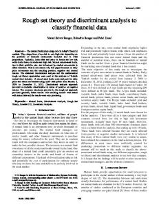
We analysed the distribution of the minimum 𝑀𝑢 (𝑘) values, per employer, and per 𝑦̂,𝑦 job over all units (employers, jobs) in the sample. The minimum 𝑀𝑢 (𝑘) values at employer level (Figure 1) tend to be somewhat larger than those at job level (Figure 2). Most of the minimum values at employer level are within the range of 0-4, whereas most of the minimum values at job level are within 0-2. Furthermore, both 𝑦̂,𝑦 at employer-level and at job-level the distribution of the minimum 𝑀𝑢 (𝑘) values 𝑦̂,𝑦 show two peaks, with a dip between the peaks at a value of about 𝑀𝑢 (𝑘) =1.
𝑦̂,𝑦
Figure 1. Distribution of the minimum value for 𝑀𝑖 (𝑘) per employer, for 2011 (left) and 2012 (right).
𝑦̂,𝑦
Figure 2. Distribution of the minimum value for 𝑀𝑗 (𝑘) per job, for 2011 (left) and 2012 (right).
CBS | Discussion Paper 2015 | Klik hier om het reeksnummer in te voeren.
20
Next, we did a sensitivity analysis on the value of the threshold 𝑇0𝑢 for indicator 𝑦̂,𝑦 𝑀𝑢 (𝑘) on three groups of patterns: the fraction of units for which no pattern could 𝑦̂,𝑦 be appointed, thus 𝑀𝑢 (𝑘)> 𝑇0𝑢 ) (labelled as UNK), the fraction of units that report the same value each month (pattern 5 and 6: labelled as AVG) and the fraction of units with any other pattern (labelled as OTHER). Note that the fractions UNK, AVG and OTHER add up to 1. We limited the sensitivity analyses to the 2011 data, and did the analyses for both the employer-level regressions and the job-level regressions.
𝑦̂,𝑦
Figure 3. Sensitivity analyses on the threshold 𝑇0𝑢 for indicator 𝑀𝑢 (𝑘) at employerlevel (left) and at job level (right). For the employer-level regressions a threshold value of 0 resulted in 80 per cent of the employers for which no pattern was appointed (UNK), thus for 20 per cent of the employers we appoint a pattern for which we found a perfect regression fit. For those units we are absolutely sure that we appoint the correct pattern to all sampled jobs underlying that (sampled) employer. Likewise, at job-level, a threshold value of 0 resulted in 46 per cent of the jobs for which no pattern was appointed (UNK) thus 54 per cent of the jobs were appointed a pattern for which we found a perfect fit. In other words, at employer-level (fitting multiple jobs at once) we had far less cases of perfect fits than at job level. Data inspection showed that within one employer, there usually were a few cases with deviating values. (see Table 13 and Table 14 for examples) 𝑦̂,𝑦
When the threshold value for 𝑀𝑢 (𝑘) was increased from 0 to 5 the relative number of records for which no patterns was appointed (UNK) dropped to 10 per cent (employer-level) and 7 per cent (job-level). In other words, 90 per cent (employer) and 93 per cent (job-level) of the units had a mean absolute prediction error of at most 5%. A prediction error of at most 5 per cent appears to be small, but the temporal patterns that we investigated (the relative values of the different regressors) did not differ much from each other. Recall that we tested only a 𝑦̂,𝑦 selection of (known) patterns. That implies that when 𝑀𝑢 (𝑘) = 5, there is a considerable risk that the true pattern is not the pattern that, within our regressions 𝑦̂,𝑦 has the minimum value for 𝑀𝑢 (𝑘), but another pattern not yet included in our options list in table 1 that, when tested, would have produced a smaller value for 𝑦̂,𝑦 𝑀𝑢 (𝑘). CBS | Discussion Paper 2015 | Klik hier om het reeksnummer in te voeren.
21
Figure 3 further shows that pattern AVG increased from 12 to 37 per cent (employerlevel) and from 34 to 46 per cent (job level) of the units when the threshold value increased from 0 to 5. So with increasing prediction error, considerably more units are appointed to the AVG pattern. We are not sure whether those units truly have the AVG pattern, maybe the increasing prediction error in fact means that they should be appointed to another pattern that was not included into our regressions. For the test set it is more important that we are (nearly) sure that the patterns that we appoint are correct than that we have a large proportion of records with an appointed pattern. We therefore choose to use a small threshold value. We selected 𝑦̂,𝑦 this threshold value as follows. Consider the distribution of the minimum 𝑀𝑗 values per job over all jobs in the sample. Now, we set the threshold value such that at most 𝑦̂,𝑦 𝑦̂,𝑦 5 per cent of the (minimum) 𝑀𝑗 values are in the range 0 < 𝑀𝑗 ≤ 𝑇0𝑗 . Note that we excluded the values 𝑇0𝑗 = 0, because for those values we are already sure that we select the correct pattern. We found the threshold value 𝑇0𝑗 = 0.04, corresponding to 5.1% (2011) and 5.3% (2012) of the minimum values in the range 𝑦̂,𝑦 0 < 𝑀𝑗 ≤ 𝑇0𝑗 . Likewise, we have the population of employers for which the corresponding jobs are in the sample. Again we set the threshold value such that at most 5 per cent of the 𝑦̂,𝑦 (minimum) 𝑀𝑖 values per employer (concerning the regressions at employer-level) 𝑦̂,𝑦 are in the range 0 < 𝑀𝑗 ≤ 𝑇0𝑗 . At a threshold of 𝑇0𝑖 = 0.08, 4.8% (2011) and 5.5% 𝑦̂,𝑦
(2012) of the minimum values were within 0 < 𝑀𝑗
≤ 𝑇0𝑗 .
CBS | Discussion Paper 2015 | Klik hier om het reeksnummer in te voeren.
22
Table 7 Number of records in the sample that was appointed outside the test set (column "No") or inside the test set ("Yes"), counted at employer-level, for regressions at job-level 2011
Sector
A
No
Yes total
2092
412
2012 Yesperfect fit 275
No
2035
Yes Yes total Perfect fit 447 316
B
106
71
58
95
67
53
C
1721
480
246
1771
476
213
D
79
36
28
76
32
24
E
376
91
61
385
121
64
F
1760
619
427
1720
603
415
G
2418
611
413
2443
553
349
H
1141
236
183
1096
221
143
I
2748
218
184
2682
245
208
J
1245
518
435
1305
495
389
K
1054
571
521
1040
560
516
L
1165
559
517
1152
538
487
M
1988
717
606
1927
719
602
N1
1562
322
249
1576
346
253
N2
1130
284
238
1207
255
218
O
402
123
33
382
130
27
P
1114
57
43
1127
49
39
Q
1374
44
34
1336
66
47
R
1734
306
280
1729
336
308
S
1847
466
415
1843
487
421
T
45
80
76
51
65
63
U Total
42
100
98
42
103
103
27143
6921
5420
27020
6914
5258
CBS | Discussion Paper 2015 | Klik hier om het reeksnummer in te voeren.
23
Table 8 Number of records in the sample that was appointed outside the test set (column "No") or inside the test set ("Yes"), counted at job-level, for regressions at job-level Sector
2011
No
2012
Yes Yes total perfect fit
No
Yes total
Yes perfect fit
A
2655
1247
1184
2600
1313
1240
B
1484
2473
2343
1287
2697
2520
C
1630
2311
2105
1690
2282
2056
D
1014
2963
2835
994
2979
2835
E
1546
2427
2210
1548
2428
2157
F
1923
2022
1811
1934
2018
1823
G
1890
2058
1918
1913
2019
1881
H
1992
1886
1667
1973
1925
1722
I
2888
1010
979
2881
1021
972
J
1069
2868
2729
1166
2803
2677
K
946
2970
2752
937
3039
2816
L
1402
2552
2512
1439
2519
2478
M
1138
2791
2690
1156
2799
2726
N1
2361
1530
1442
2361
1596
1485
N2
1752
1792
1707
1840
1690
1604
O
1323
2589
2425
1265
2650
2464
P
1756
2061
2036
1754
2057
2021
Q
1973
1656
1614
1950
1642
1580
R
2271
1529
1477
2205
1630
1568
S
1814
2101
2007
1864
2081
1990
T
55
114
114
58
99
99
U
185
533
529
226
582
579
35067
43483
41086
35041
43869
41293
Total
5.2 Relative frequency of the appointed patterns The relative frequencies (in per cent) of the main patterns as appointed by the employer-level regressions are given in Table 9 (relative to the number of sampled employers) and those appointed at job-level are given in Table 10 (relative to the number of sampled jobs). The most frequently occurring main pattern is AVG (reporting the same value each month). That pattern was appointed to 13.7 per cent of the employers and to 35.9 per cent of the jobs, as averaged over the economic sectors and over the two years. The second most frequent pattern is WDS (working days), that was, on average, appointed to 9.3 per cent of the employers and to 18.3 per cent of the jobs. All the other appointed patterns are relatively rare. In most of the cases the appointed patters concern hour paid refers to contract hours only rather than both contract and overtime hours.
CBS | Discussion Paper 2015 | Klik hier om het reeksnummer in te voeren.
24
There is a considerable variation in the frequency of appointed patterns across economic sectors. In sector I, P and Q less than 10 per cent of the sampled employers were appointed a pattern. At job-level, sector I also had the smallest percentage of appointed to a pattern (26%). Sector P and Q however had much larger percentages at job level. This means that in sector P and Q some employees within an employer have a well-known pattern whereas others deviate. In sector I however, all jobs deviate from the investigated patterns. At the other end of the spectrum in sector U 70.7 per cent of the employers and 73.1 of the jobs were appointed a pattern (with WDS and AVG as the dominating patterns). That means that sector U relatively nicely coincides with the tested patterns. The patterns where hours paid concerns both regular and overtime hours were appointed relatively most often in sector O (public administration and defence), at least when tested at employer-level. Overtime-hours is typically investigated easier at employer level that at job-level, since it can only be detected for those employees that had overtime. A final example of a pattern that clearly varies across sectors is CAL (calendar days). This rare pattern was appointed mainly in the sectors B and T (both at employer and job level) and N1 (at job level).
Table 9 Relative pattern frequency as averaged over 2011 and 2012 at employerlevel, abbreviations refer to Table 2. Sect.
ZRO
ONE AVG- AVG+ VWK- VWK+ CAL* WDS- WDS+ OWK
UKN
A
0.4
0.2
5.4
0.7
0.1
0.0
0.0
9.3
1.0
0.0
82.8
B
0.6
0.3
17.4
5.3
0.0
0.0
0.6
14.4
2.1
0.0
59.3
C
0.3
0.0
8.3
8.0
0.1
0.0
0.0
3.1
1.7
0.0
78.5
D
1.8
0.0
10.3
6.3
0.0
0.0
0.0
11.2
0.9
0.0
69.5
E
0.2
0.0
7.5
5.7
0.0
0.0
0.0
6.1
2.3
0.0
78.3
F
1.3
0.1
10.7
2.8
0.5
0.0
0.0
8.4
2.3
0.0
74.0
G
0.4
0.0
9.1
4.4
0.0
0.0
0.0
4.6
0.8
0.0
80.7
H
0.9
0.0
6.7
3.5
0.0
0.0
0.0
5.0
0.9
0.0
83.0
I
0.3
0.0
5.2
0.1
0.0
0.0
0.0
2.2
0.1
0.0
92.1
J
1.4
0.1
13.0
3.1
0.0
0.0
0.0
9.6
1.2
0.0
71.6
K
3.1
0.7
19.4
1.6
0.1
0.0
0.0
9.9
0.2
0.0
64.9
L
2.0
0.4
18.3
1.3
0.0
0.0
0.0
10.0
0.2
0.0
67.9
M
1.5
0.3
13.6
2.5
0.0
0.0
0.0
8.1
0.7
0.0
73.2
N1
0.9
0.1
8.0
1.8
0.1
0.0
0.0
5.9
0.8
0.0
82.5
N2
1.8
0.3
7.3
1.3
0.2
0.0
0.0
6.6
1.3
0.0
81.2
O
0.2
0.0
7.1
17.1
0.0
0.0
0.0
0.0
0.0
0.0
75.6
P
0.5
0.1
2.6
0.4
0.0
0.0
0.0
0.7
0.2
0.0
95.5
Q
0.3
0.0
2.3
0.7
0.0
0.0
0.0
0.6
0.0
0.0
96.1
R
1.0
0.2
9.2
0.7
0.0
0.0
0.0
4.4
0.1
0.0
84.4
S
0.8
0.2
13.6
1.4
0.1
0.0
0.0
4.2
0.2
0.0
79.5
T
3.3
0.0
39.8
0.0
0.0
0.0
2.1
14.9
0.0
0.0
40.0
U
0.7
0.0
21.3
0.4
0.0
0.0
0.0
48.0
0.4
0.0
29.3
Mean
1.1
0.1
11.6
3.1
0.1
0.0
0.1
8.5
0.8
0.0
74.5
CBS | Discussion Paper 2015 | Klik hier om het reeksnummer in te voeren.
25
Table 10 Relative pattern frequency as averaged over 2011 and 2012 at job-level, abbreviations refer to Table 2. Sect. A B C D E F G H I J K L M N1 N2 O P Q R S T U Mean
ZRO 0.5 0.4 0.7 0.1 0.4 1.3 0.8 1.8 0.4 1.6 2.3 2.1 1.6 1.0 2.8 2.0 0.9 1.3 1.8 2.4 3.6 1.8 1.4
ONE AVG- AVG+ VWK- VWK+ CAL* WDS- WDS+ OWK 0.3 12.2 0.7 0.3 0.0 0.0 17.3 1.5 0.0 0.1 25.1 4.8 0.0 0.1 4.7 29.2 0.5 0.1 0.1 36.1 4.9 0.3 0.1 0.0 13.9 1.8 0.1 0.1 46.1 3.6 0.0 0.1 0.0 24.1 0.6 0.1 0.0 39.5 6.9 0.0 0.2 0.0 12.4 1.6 0.1 0.1 23.4 3.7 1.1 0.1 0.0 19.4 2.2 0.0 0.2 28.8 2.6 0.1 0.2 0.0 17.5 1.5 0.0 0.1 31.3 5.5 0.1 0.1 0.0 8.5 1.5 0.1 0.1 17.1 0.7 0.2 0.0 0.0 7.3 0.2 0.0 0.1 34.9 2.8 0.0 0.1 0.0 30.3 1.8 0.0 0.4 50.0 3.2 0.2 0.1 0.0 19.2 0.8 0.0 0.5 35.6 1.1 0.1 0.1 0.0 24.2 0.4 0.0 0.3 33.8 1.7 0.1 0.1 0.1 32.0 1.3 0.0 0.2 19.8 1.3 0.2 0.0 0.6 14.9 1.7 0.0 0.4 24.4 1.7 0.4 0.1 0.0 17.5 1.9 0.0 0.1 57.6 6.4 0.0 0.2 0.0 0.6 0.1 0.1 0.1 50.2 0.4 0.0 0.0 0.1 2.1 0.1 0.0 0.1 38.9 1.7 0.0 0.1 0.0 3.4 0.2 0.0 0.4 24.4 1.2 0.1 0.1 0.0 13.0 0.4 0.1 0.2 34.4 1.7 0.3 0.1 0.0 13.4 0.5 0.1 0.0 39.9 0.0 0.0 0.0 1.2 20.6 0.0 0.0 0.4 29.7 0.1 0.0 0.0 0.0 41.2 0.0 0.0 0.2 33.3 2.6 0.1 0.1 0.3 17.4 0.9 0.0
UKN 67.2 34.9 42.0 25.3 38.9 48.8 48.3 51.0 74.0 28.3 23.9 35.9 29.1 60.2 50.8 33.1 46.0 54.3 58.6 46.8 34.7 26.9 43.6
5.3 Comparing the employer-level with job-level patterns So far, we presented the results of the employer-level regression in terms of the percentage of (sampled) employers that are appointed to a specific pattern whereas the result of the job-level regressions are expressed in terms of the percentage of (sampled) jobs that are appointed to a specific pattern. We also directly compared the result of both approaches, see Table 11. In Table 11 we consider the set of jobs in the original sample and we count the numbers appointed to a pattern according to both approaches. Table 11 shows that when we appoint a job to the test set (thus classifying the record to one of the possible patterns), according to the employer level regression, we nearly always appointed this job to the test set according to the job-level regression, but not the other way around. A similar result is obtained when we counted the main patterns AVG and WDS (in both years). The explanation for this result is that usually a few outlying observations (in one or two employers of the extended sample) lead to a relatively large value of the M-indicator at employer-level. At job-level however, we classify one job at a time, so a large part of the jobs could be classified. For the final test set we use two-step approach, we first appoint the jobs to the pattern of the employer-level regression. The remaining, non-classified records are then appointed to the job-level regression (if any). CBS | Discussion Paper 2015 | Klik hier om het reeksnummer in te voeren.
26
Table 11 Number of jobs in the sample appointed to a patterns according to joblevel versus employer level regression Employer-level
Job-level 2011
2012
Appointed to any pattern yes
no
yes
no
yes
10682
32801
10555
33314
no
724
34343
837
34204
Pattern AVG yes
7211
21081
7415
20982
no
401
49857
513
50000
Pattern WDS yes
2371
11050
2231
11722
no
560
64569
539
64418
6. Discussion The present paper deals with WS-data on hours worked and wage components per job of employees. These data are used estimate the total number of hours worked per month and hourly wages classified by job, employer and enterprise characteristics. These WS-data concern administrative data that are reported by employers to the tax office at different frequencies. The monthly reporters have a large number of different temporal reporting patterns , especially so for the variable hours paid. Since there is no variable in the data set explaining which patterns is used, Statistics Netherlands needs to detect these patterns ourselves. In the current statistical production system a regression method (slightly different from the current study) is used to detect those patterns, but still about one-third of the jobs cannot be classified. In the long rum we want to classify all jobs that report monthly values of hours paid into a reporting pattern. To that end wish to investigate whether data mining methods are suitable for this purpose. Data mining methods often require a test set of records with a known (labelled) pattern in order to test the efficacy of the method. The current study aimed to derive such a test set. In accordance with earlier studies (Jansen et al., 2012; Moerman, 2015), we identified (in the sampled WS-data) a number of typical patterns in the reporting of the hours paid. Those reporting patterns are in line with the rules set by the terms of the official declaration regulations but they hamper a correct computation of the hourly wages by Statistics Netherlands. Typical temporal reporting patterns also occur in the Dutch Value Added tax data (Ouwehand, 2011; van Delden and de Wolf, 2013). In Dutch VAT data businesses report their turnover on a monthly, quarterly or yearly CBS | Discussion Paper 2015 | Klik hier om het reeksnummer in te voeren.
27
frequency. In typical economic sectors, e.g. supermarkets, the businesses run an administration on a four-week basis. The values they report that officially concern a month, in fact concern four-week values, likewise for the VWK pattern in hours paid (van Delden and de Wolf, 2013). Besides these four-week patterns all kinds of other patterns exist. In the case of the tax data, we are interested in the estimation of monthly growth figure of aggregates, and for that purpose, the effects of the different patterns cancel out (Ouwehand, 2011). We succeeded in appointing about 56 per cent of the sampled jobs to a pattern of which we are very sure that we have the correct one and that can thus be used as a test set. We encountered a number of issues that made it difficult to appoint a pattern. First of all, some of the different (sub)patterns appear very similar as long as you consider only one year of data at the same time. For instance, the sub patterns within the WDS patterns are similar. We may investigate in future whether it is easier to identify the patterns when we use longer time series. Note that when the patterns completely overlapped (e.g. hours paid varies with number of mondays-fridays per month and the number of Social Insurance days is identical to the number of Mondays-Fridays) we chose to count the most specific pattern. The actual choice that we made is not really important, as long as we keep this in mind when we use the test set for next steps. While it might appear that the percentage of jobs that we can assign a pattern to with certainty is small, this could be due in part to the fact that our 'dictionary' of possible patterns (table 1) is incomplete. For instance, when somebody follows one of the patterns that we tested for, but somewhere during the year this person increased or decreased its number of working hours we did not detect this pattern. A second issue is the presence of outlying values in the WS-data that are probably measurement errors. That makes it difficult to appoint the correct patterns. We noticed this in particular when comparing the employer-level results with the joblevel regressions. The robust version of the mean absolute prediction error, that included Huber weights, was not really suitable as an indicator to select the records that are likely to belong to a pattern. In future work, we need to develop an indicator that can handle the typical outliers of our data set in the correct way. One possible option is to drop months from the computation of the prediction error, for the months with the smallest Huber weights (< 1), up to a maximum of e.g. three months. A third issue concerns the number of data points (dependent variable is 'number of hours worked', the independent variable is for instance the 'number of working days in a month') that is available for each job. Although we used twelve months of data for each job, we often had only three to five different values for the independent variable. That makes the regression approach less suitable for our pattern recognition. Since we are most interested in methods that allow us to detect unknown patterns and new patterns (in case they emerge), unsupervised learning methods appear to be the most logical candidate (Hastie et al., 2009). This hopefully also offers the opportunity to identify more sub patterns than were included in our study.
CBS | Discussion Paper 2015 | Klik hier om het reeksnummer in te voeren.
28
7. Literature Delden, A. van and P.P. de Wolf (2013). A production system for quarterly turnover levels and growth rates based on VAT data. Paper presented at the NTTS Conference, 5–7 March 2013, Brussels Hastie, T., Tibshirani, R. and J. Friedman (2009). The elements of statistical learning. Springer-Verlag. (2009 edition). Hand, D.J. (1998). Data mining statistics and more? The American Statistician, Vol. 52, No. 2 (May, 1998), pp. 112-118. Jansen, N., Huijsmans, N. and M. Heerschop (2012). [in Dutch] Kwaliteitsonderzoek naar het gegeven Verloonde Uren. Nota UWV en CBS. (in Dutch) Neter, J. Kutner, M.H. , Nachtsheim, C.J. and W. Wasserman, Applied linear statistical models. Fourth edition. Irwin, Chicago, 1996. Moerman,, E. (2015). [in Dutch] Overzicht kwaliteit van verloonde uren. Notitie van het UWV. Ouwehand, P. and Delden, A. Van (2011). [in Dutch] Revisions after correction of systematic errors. CBS report, DMV 2011-06-29-PWOD-ADLN
Acknowledgements The authors like to thank Jan van der Laan for his help with the R code and Sander Scholtus for his help with the regression approach. Furthermore, we thank Mark Hartog van Banda, Michiel Heerschop and Henrico Witvliet, for their help with the data and with understanding the reporting patterns.
CBS | Discussion Paper 2015 | Klik hier om het reeksnummer in te voeren.
29
8. Appendix 8.1 Pattern examples Explanation for Table 12. Time variable (TV), hours paid (HP), wages overtime (WO). The time variable that is shown depends on the pattern: for CAL pattern TV equals calendar days, for Pat 27 TV equals number of Mondays, Tuesdays, Thursdays and Fridays; for SID pattern, TV equals the number of SID days. Table 12 Examples of (sub)patterns 2011 at job-level Month TV
HP
WO
AVG no overtime 1
-
TV
HP
WO
AVG & overtime
30
0
2
30
0
87
3
30
0
4
30
5
30
6
TV
HP
WO
CAL - exact
HP
WO
CAL - not exact
31
248
0
31
151
0
0
28
224
0
28
137
0
87
0
31
248
0
31
151
0
0
87
0
30
240
0
30
146
0
0
87
0
31
248
0
31
151
0
30
0
87
0
30
240
0
30
146
0
7
30
0
87
0
31
248
0
31
151
0
8
30
0
87
0
31
248
0
31
151
0
9
30
0
87
0
30
240
0
30
146
0
10
30
0
87
0
31
248
0
31
151
0
11
30
0
87
0
30
240
0
30
146
0
12
30
0
87
0
31
248
0
31
151
0
Pat27-exact
135 930
TV
Pat27- not exact
SID-exact
SID-not exact
1
17
136
0
17
122
0
8
64
0
13
110
0
2
16
128
0
16
115
0
8
64
0
12
102
0
3
18
144
0
18
129
0
9
72
0
13
110
0
4
17
136
0
17
122
0
9
72
0
13
110
0
5
18
144
0
18
129
0
8
64
0
13
110
0
6
17
136
0
17
122
0
9
72
0
13
110
0
7
17
136
0
17
122
0
9
72
0
13
110
0
8
18
144
0
18
129
0
9
72
0
14
119
0
9
18
144
0
18
129
0
9
72
0
13
110
0
10
17
136
0
17
122
0
8
64
0
13
110
0
11
17
136
0
17
122
0
9
72
0
13
110
0
12
18
144
0
18
129
0
9
72
0
13
110
0
CBS | Discussion Paper 2015 | Klik hier om het reeksnummer in te voeren.
30
Table 13 Example of pattern (2011) for one employer Job
Month
HP
WO
SID
1
1
60
0
17
1
2
60
0
17
1
3
60
0
17
1
4
60
0
17
1
5
60
0
17
1
6
120
0
17
1
7
60
0
17
1
8
60
0
17
1
9
60
0
17
1
10
60
0
17
1
11
60
0
17
1
12
60
0
17
2
1
30
0
9
2
2
30
0
9
2
3
30
0
9
2
4
30
0
9
2
5
30
0
9
2
6
30
0
9
2
7
30
0
9
2
8
30
0
9
2
9
30
0
9
2
10
30
0
9
2
11
30
0
9
2
12
30
0
9
CBS | Discussion Paper 2015 | Klik hier om het reeksnummer in te voeren.
31
Table 14 Example of pattern (2011) for another employer. Sample
Job
Mn
HP
Sample
Job
Mn
HP
FALSE
1
1
152 0
WO SID 0
FALSE
3
1
134 0
WO SID 21
FALSE
1
2
152 0
0
FALSE
3
2
134 0
20
FALSE
1
3
152 0
0
FALSE
3
3
134 0
23
FALSE
1
4
152 0
0
FALSE
3
4
134 0
21
FALSE
1
5
152 0
0
FALSE
3
5
134 0
22
FALSE
1
6
152 0
0
FALSE
3
6
17
0
5
FALSE
1
7
152 0
0
FALSE
3
7
17
0
4
FALSE
1
8
152 0
0
FALSE
3
8
17
0
5
FALSE
1
9
152 0
0
FALSE
3
9
17
0
4
FALSE
1
10
152 0
0
FALSE
3
10
17
0
4
FALSE
1
11
152 0
0
FALSE
3
11
17
0
5
FALSE
1
12
152 0
0
FALSE
3
12
17
0
4
FALSE
2
1
17
0
4
TRUE
4
1
17
0
4
FALSE
2
2
17
0
4
TRUE
4
2
17
0
4
FALSE
2
3
17
0
5
TRUE
4
3
17
0
5
FALSE
2
4
17
0
4
TRUE
4
4
17
0
4
FALSE
2
5
17
0
4
TRUE
4
5
17
0
4
FALSE
2
6
17
0
5
TRUE
4
6
17
0
5
FALSE
2
7
17
0
4
TRUE
4
7
17
0
4
FALSE
2
8
17
0
5
TRUE
4
8
17
0
5
FALSE
2
9
17
0
4
TRUE
4
9
17
0
4
FALSE
2
10
17
0
4
TRUE
4
10
17
0
4
FALSE
2
11
17
0
5
TRUE
4
11
17
0
5
FALSE
2
12
17
0
4
TRUE
4
12
17
0
4
CBS | Discussion Paper 2015 | Klik hier om het reeksnummer in te voeren.
32
8.2 Number of sub patterns at employer-level Table 15 Number of sub patterns 2011 at employer-level, numbers refer to Table 2. BK
1
3
5
6
7
8
12
13
14
A
10
4
129
17
3
0
0
0
B
1
1
30
9
0
0
0
0
C
7
0
205 161
1
0
0
D
3
0
0
0
E
1
F
29
G
19
21
22
25
0
0 218
31
0
0
1
27
2
0
1
0
0
65
39
1
0
0
0
0
15
0
0
12
6
0
33
17
0
0
0
0
0
0
30
10
0
3
251
59
15
1
0
0
0
0 205
56
0
17
3
283 135
1
0
0
0
0
0 148
24
0
H
13
0
108
34
0
0
0
0
0
0
72
9
0
I
13
1
136
3
0
0
0
0
0
0
64
1
0
J
28
4
238
45
0
0
0
0
0
0 181
22
0
K
58
9
306
25
2
0
0
0
0
0 165
6
0
L
38
5
314
22
0
0
0
0
0
0 178
2
0
M
41
10
367
66
0
1
0
0
0
0 209
23
0
N1
19
3
154
31
2
0
1
0
0
0
98
14
0
N2
33
6
110
17
4
0
0
0
0
0
94
20
0
O
1
0
39
83
0
0
0
0
0
0
0
0
0
P
8
1
33
4
0
0
0
0
0
0
8
3
0
Q
5
0
25
7
0
0
0
0
0
0
7
0
0
R
17
4
179
11
0
0
0
0
0
0
91
3
1
S
21
4
308
24
0
0
0
2
1
0 105
1
0
T
6
0
51
0
0
0
0
0
0
3
20
0
0
U
1
0
34
1
0
0
0
0
0
0
63
1
0
2.6 152.0 35.3
1.3
0.1
0.0
0.1
0.0
0.2 93.8 12.1
0.1
Mean 16.8
CBS | Discussion Paper 2015 | Klik hier om het reeksnummer in te voeren.
33
Table 16 Number of sub patterns 2012 at employer-level, numbers refer to Table 2. BK
1
3
5
6
7
8
9
13
A
11
4
142
19
2
0
2
B
1
0
29
9
0
0
C
5
0
165 197
1
D
1
0
11
8
E
1
0
40
39
F
31
1
251
G
7
0
H
12
1
72
I
5
1
168
J
23
0
K
42
L M
19
21
22
25
0
0 246
21
0
0
0
1
22
5
0
0
0
0
0
69
38
1
0
0
0
0
0
10
2
0
0
0
0
0
0
29
12
0
71
7
1
1
0
0 189
51
0
266 129
0
0
0
0
0 128
23
0
59
0
0
0
0
0
62
15
0
4
1
0
0
0
0
63
3
0
225
65
0
0
0
0
0 160
22
0
14
321
27
0
0
1
0
0 154
1
0
29
7
310
23
0
0
0
0
0 163
6
0
38
7
363
69
0
0
1
1
0 223
17
0
N1
14
1
152
37
0
0
1
1
0 125
15
0
N2
19
2
99
20
1
1
0
0
0
96
17
0
O
1
0
35
94
0
0
0
0
0
0
0
0
P
4
1
28
5
0
0
0
0
0
9
2
0
Q
3
1
39
13
0
0
0
0
0
10
0
0
R
26
5
198
18
0
0
0
0
0
88
1
0
S
18
3
323
42
0
0
0
3
0
92
6
0
T
2
0
45
0
0
0
0
0
2
16
0
0
U
1
0
27
0
0
0
0
0
0
75
0
0
Mean 13.4 2.18 150.4 43.1 0.55 0.09 0.27 0.23 0.14 92.2 11.7 0.05
CBS | Discussion Paper 2015 | Klik hier om het reeksnummer in te voeren.
34
8.3 Number of sub patterns at job-level Table 17 Number of sub patterns 2011 at job-level, numbers refer to Table 2.
CBS | Discussion Paper 2015 | Klik hier om het reeksnummer in te voeren.
35
Table 18 Number of sub patterns 2012 at job-level, numbers refer to Table 2.
CBS | Discussion Paper 2015 | Klik hier om het reeksnummer in te voeren.
36
Explanation of symbols Empty cell . * **
Figure not applicable Figure is unknown, insufficiently reliable or confidential Provisional figure Revised provisional figure
2015–2016
2015 to 2016 inclusive
2015/2016
Average for 2015 to 2016 inclusive
2015/’16 2013/’14–2015/’16
Crop year, financial year, school year, etc., beginning in 2015 and ending in 2016 Crop year, financial year, etc., 2013/’14 to 2015/’16 inclusive Due to rounding, some totals may not correspond to the sum of the separate figures.
Publisher Statistics Netherlands Henri Faasdreef 312, 2492 JP The Hague www.cbs.nl Prepress CCN Creatie, The Hague Design Edenspiekermann Information Telephone +31 88 570 7070 Via contact form: www.cbs.nl/information © Statistics Netherlands, The Hague/Heerlen/Bonaire, 2016. Reproduction is permitted, provided Statistics Netherlands is quoted as the source.
CBS | Discussion Paper, 2016 | 16 37