Design and Deployment of a Continuous Monitoring System for the Dowling Hall Footbridge Peter Mosera and Babak Moavenib Abstract
Continuous monitoring of structural vibrations is becoming increasingly common as interest in structural health monitoring (SHM) grows, as equipment becomes more affordable, and as system and damage identification methods develop. In vibration-based SHM, the dynamic modal parameters of a structure may be used as damage-sensitive features. The modal parameters are often sensitive to changes in temperature or other environmental effects so continuous monitoring systems must also measure environmental conditions. Necessary components of a continuous structural monitoring system include a well-designed sensor array, data acquisition and logging equipment, data transfer and storage functions, and routines for extracting modal parameters from vibration measurements. All processes must be automated to handle the large volume of data generated. Such a monitoring system has been installed on the Dowling Hall Footbridge at Tufts University and is currently providing live data for research in vibration-based SHM. This paper focuses on (1) the design and installation of the system hardware and (2) the strategy used to automate the monitoring system. Successful automation of modal analysis is emphasized as the key component of this strategy. To highlight the system’s capabilities, the pattern of variation of the natural frequencies is examined and compared with environmental data.
Introduction
Major structural failures in recent years have brought the need for improved infrastructure monitoring and maintenance to public attention1. The nation’s roadways include more than 600,000 bridges2 which are normally monitored by visual inspections; maintenance is performed when judged necessary. In many cases, accurate assessment of a bridge’s condition is not really possible by these visual inspections. The American Society of
a
Graduate student, Dept. of Civil and Environmental Engineering, Tuft University, Medford, MA. E‐mail:
[email protected] b Assistant Professor, Dept. of Civil and Environmental Engineering, Tuft University, Medford, MA. E‐mail:
[email protected] (corresponding author), telephone: 617‐627‐5642, fax: 617‐627‐3994 1
Civil Engineers issued its Report Card for America’s Infrastructure in 20093, giving bridges an overall grade of “C.” A key statistic determining this grade is the number of bridges classified as either “structurally deficient” or “functionally obsolete.” Nationwide, more than 26% of bridges fall into at least one of these classifications. To reduce the number of deficient and obsolete bridges, ASCE recommends increased spending on maintenance and construction, more balanced and intelligent management of existing resources, updated inspection standards and risk-based prioritization for maintenance, and increased funding for transportation research. Structural health monitoring (SHM) of the nation’s bridge system can help to meet these goals by providing accurate, timely, and objective information about the condition of a bridge4. The advantages of a SHM system include early warning if a bridge becomes unsafe, the capability to locate and quantify damage in a bridge, and better targeting of maintenance resources by identifying which structures most need maintenance. Continuous vibration monitoring is one strategy for SHM. In such a monitoring system, the vibrations of a bridge due to traffic, wind, and other ambient sources are measured and recorded. From these vibration records, the dynamic modal parameters (natural frequencies, damping ratios, and mode shapes) of the structure can be determined using operational modal analysis techniques. Once the modal parameters have been determined they can be used for condition assessment. A typical damage scenario involves loss of stiffness in some portion of the structural system and a corresponding change in the modal parameters. Automatic modal analysis is central to a continuous monitoring system. The basic function of modal analysis is to estimate the modal parameters from a measured vibration record. Two popular output-only time-domain methods for extracting modal parameters from ambient vibrations are the Natural Excitation Technique5 combined with the Eigensystem Realization Algorithm6 (NExT-ERA) and data-driven Stochastic Subspace Identification7 (SSI-Data). Automation of these identification methods requires a technique to distinguish between true modes of the system and the “mathematical” or “noise” modes which may also be identified. A stabilization diagram8 is often used for this purpose. Using this strategy, modal analysis can be completely automated with accurate results9. The goal of vibration-based SHM is to use the modal parameters for damage identification. However, modal parameters can be affected by factors other than damage. Temperature and humidity affect material properties10,11 and boundary conditions12. Large volumes of traffic can change a structure’s mass13,14. In a nonlinear structure, dynamic properties change with excitation amplitude15. All these factors can influence the
2
modal parameters of a bridge but temperature is the most commonly considered environmental variable16. It has been shown that modal parameters are sensitive not only to changes in temperature, but also to gradients in temperature along the structure17,18. Changes in natural frequency in the order of 10% from these sources are not unusual18,19. A continuous monitoring system must account for these changes if it is to accurately and reliably identify damage. This paper presents the details of a vibration-based continuous monitoring system deployed on the Dowling Hall Footbridge at Tufts University in Medford, MA. This system includes an array of eight accelerometers and ten thermocouples, a rugged and remotely operable data acquisition system, a reliable communication system, and fully automated modal analysis programs. The design, installation, and analysis processes are described in detail and results from the system are highlighted. The system continues to provide live data for structural health monitoring research.
Dowling Hall Footbridge
Bridge Structure
The Dowling Hall Footbridge, shown in Figure 1, is a pedestrian bridge located on the Medford, MA campus of Tufts University. The bridge is 44 m (144 ft) long and 3.7 m (12 ft) wide. This two-span continuous steel frame bridge connects the main campus with the student services offices on the seventh floor of Dowling Hall. The structural frame of the bridge is constructed of steel tubing ranging from HSS 10x4x5/16 to HSS 10x6x3/8. The structural frame on each side of the bridge also serves as the railing. The walkway is constructed of poured concrete on corrugated steel. The concrete walkway is equipped with a snowflake sensor and a piped-glycol heating system to prevent snow and ice buildup on the deck during winter months. The bridge is supported by an abutment on the west side and by tall steel/masonry piers at the center point and on the east side. Figure 2 shows a cross-section of the footbridge. More details about the Dowling Hall Footbridge can be found in Bowman (2003)20. The Dowling Hall Footbridge is well-suited for a continuous monitoring system for several reasons. The bridge is flexible and significantly excited by pedestrian traffic or wind; vibrations are easily measured and can be felt by an observer standing on the bridge. The bridge is exposed to a wide range of environmental conditions and is large
3
enough to exhibit complex structural behavior; this provides an opportunity for a realistic assessment of environmental effects. The heating system in the concrete deck provides an additional level of complexity to this aspect. The site is easily accessible from the Tufts campus and maintenance of the monitoring system does not require disrupting traffic as is often the case with bridges on public roads. The campus wireless network covers the entire area, providing some of the communication structure needed.
Figure 1. Dowling Hall Footbridge (photo on the right from )
TS10x6x3/8 0.15m TS8x6x5/16 64mm concrete on 38mm steel cellular deck
1.63m
C8 Channel
TS10x6x5/16
0.25m
0.15m TS10x4x5/16 @ 2.44m O.C. 0.25m
3.61m
0.25m
Figure 2. Cross-section of the Dowling Hall Footbridge
4
Preliminary Tests
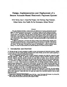
In order to properly design the continuous monitoring system, two sets of dynamic tests were performed in April and June 2009. The objective of these tests was to determine the natural frequencies and mode shapes of the bridge and assess the level of bridge response amplitudes due to ambient excitation. These tests used twelve accelerometers temporarily fixed to the top of the bridge deck using metal mounting brackets and epoxy. Their results are briefly summarized below. A test on April 4, 2009 was performed to assess both the vertical and horizontal vibrations of the bridge. During the vertical vibration tests, twelve sensors (six on the north edge and six on the south edge of the deck) were used to measure the vertical component of bridge response. System identification was performed by the SSI-Data algorithm. Figure 3 shows the first six identified vertical mode shapes with their natural frequencies. Note that the mode shapes shown were drawn assuming no motion at the supports (indicated by black circles). The identified space-discrete mode shapes were interpolated between the sensor locations (indicated by empty circles) using cubic spline interpolation. In the horizontal tests, vibrations were detectable but much smaller in magnitude than their vertical counterparts. A follow-up test was conducted on June 4, 2009 to assess the motions at the supports. Motion at supports was measurable but generally small. The largest motion occurred at the tall pier on the east side, nearest to Dowling Hall, consistent with the increased flexibility of the tallest pier. Even at this pier the motion is less significant than motion between supports. Based on these preliminary tests it was decided that the continuous monitoring system should measure vertical motions only and that measurements at the supports were unnecessary. It was further concluded that the primary frequencies of interest were between 2 and 20 Hz. Knowledge of the mode shapes allowed planning of sensor locations to avoid modal nodes.
Continuous Monitoring System
A vibration-based continuous monitoring system was designed for the Dowling Hall Footbridge based on results of initial testing. The system was designed during the summer of 2009 and installed on the bridge in November 2009.
5
f = 4.66 Hz
f = 6.21 Hz
44
f = 7.08 Hz
44 22 x [m]
44 22 x [m]
0 y [m]
f = 8.88 Hz
f = 13.23 Hz
44
0 y [m]
f = 13.62 Hz
44 22 x [m]
22 x [m]
0 y [m]
44 22 x [m]
0 y [m]
0 y [m]
22 x [m]
0 y [m]
Figure 3. Mode Shapes Identified from a Preliminary Test on April 4, 2009 Accelerometers
PCB Piezoelectronics model 393B04 uniaxial accelerometers were selected as the vibration sensors. This model features 3 µg RMS broadband resolution, a frequency range of 0.06 to 450 Hz, integrated signal conditioning, small size (25 x 31 mm), and light weight (50 grams). The operating temperature range of -18 to +80 °C and an available waterproof option make the sensor ideal for outdoor applications. The sensors were mounted to aluminum L-brackets via machine screws. The brackets were fixed to the underside of the bridge using metal/concrete epoxy. Eight uniaxial accelerometers were permanently mounted to the underside of the bridge (Figure 4). The layout of the eight accelerometers is shown in Figure 5. It is worth noting that use of more accelerometers (especially on the East span of the footbridge) would provide more spatially refined mode shape estimates that could provide more refined localization of damage. However, instrumentation of the East span (Dowling Hall side) was outside of the project capabilities due to the height above ground (~18 m) and steeply sloping terrain. The current sensor network was found adequate for estimating the six lower vibration modes considered in this study. In addition, the number of sensors has very little impact on the accuracy of modal parameter estimates using the SSI-Data method21.
6
Figure 4. Installed Accelerometer
Dowling Hall
North 8
7 6 4 5 3 2
Upper Campus
1
Figure 5. Accelerometer Layout
The waterproof accelerometers include integrated 10-32 coaxial lead cables which connect to the data acquisition device using RG58/U coaxial extension cables. Connections between cables were waterproofed with rubber tape and a paint-on sealing compound. Cables were mounted under the bridge using adhesive mounting brackets and zip ties. Some work was required before usable signals were received reliably from all eight accelerometers. At times signals contained either unacceptably large background noise or a large number of voltage spikes. In either of these cases the first item to troubleshoot was cable connections. It is not possible to determine the cause of every difficulty but excessive cable tension near connections was a large contributing factor. After some work with the connections, all sensors began operating reliably. Accelerometers 4 and 8, with their longer cable runs, still have a lower signal-to-noise ratio than do the other sensors. 7
Temperature Sensors
The monitoring system was designed to measure the air temperature, the steel frame temperature, the temperature of the heated concrete deck, and the temperature of the piers, all at several locations. All temperature sensors in this system are type T thermocouples manufactured by Omega Engineering. Type T thermocouples can measure temperatures ranging from -250 to +350 °C and are made from copper and constantan. Omega model TJ36-CPSS-18U-6 thermocouples were chosen to monitor air temperatures. These probes were fixed to the bridge using adhesive mounting squares and zip ties. The probes were mounted to the underside of the bridge so that the tip of the probe extends well into the air below the structural members (Figure 6a). Omega model SA2C-T-SMPW-CC thermocouples were chosen to monitor steel temperatures. These self-adhesive thermocouples were mounted to the surface of the structural steel members. The sensors were further secured to the bridge by covering portions of the unit with epoxy after installation. Omega model BTH-090-T-2 1/4-60-2 thermocouples were chosen to monitor temperatures of both the heated deck and of the supporting piers. These custom probes feature a spring-loaded collar for mounting and were chosen with the heated bridge deck specifically in mind. The underside of the deck is separated from the air by 4 cm of fiberglass insulation and a metal tray. Drilling into the concrete slab was unacceptable because of the heating pipes. The spring-loaded sensors maintain firm contact between the probe and the deck. Silicone heat sink compound was used for thermal grounding. The same sensors were installed for temperature monitoring in the masonry piers (Figure 6b). The system monitors air temperature at two locations (“A1” and “A2”), steel temperature at four locations (“S1” to “S4”), pier temperature at two locations (“C1” and “C4”), and bridge deck temperature at two locations (“C2” and “C3”). The layout of the ten thermocouples is shown in Figure 7. Thermocouples were connected to the data acquisition device using twisted/shielded thermocouple extension wire. Male-female plugs were used at connection points and were covered with heat-shrink tubing. Thermocouple cables were mounted on the underside of the bridge along with the accelerometer cables.
8
(a)
(b)
Figure 6. Installed Thermocouples: (a) air thermocouple A1, (b) concrete thermocouple C1
Dowling Hall
North
S4 A2 C3
C4
S3 S2 A1 C2 S1
Upper Campus
Steel Concrete
C1
Air
Figure 7. Thermocouple Layout
Data Acquisition
The National Instruments cRIO-9074 integrated chassis/controller is the core component of the data acquisition system. The cRIO-9074 features a Field Programmable Gate Array (FPGA) chip which allows customizable access to low-level chip functions. The ability to sample different sensors at different rates (acceleration vs. temperature) and direct on-chip scaling of raw data to account for channel sensitivities are two attractive features of the FPGA. The cRIO-9074 also includes a 400MHz processor, 128MB of RAM, a 488MB solid-state storage 9
drive, eight slots for NI C-series modules, two Ethernet ports, and an operating temperature range from -20 to +55 °C. The cRIO-9074 uses the LabView RealTime operating system. Once programmed, the device can run independently of a host computer and is ideal for remote applications where reliability and autonomous operation are required. Two National Instruments NI-9234 24-bit Integrated Electronics PiezoElectric (IEPE) input modules measure the accelerometer channels. Each module monitors four accelerometer channels and supports sampling rates of up to 51.2 kHz. Software-selectable options include IEPE signal conditioning with anti-aliasing filters and timebase export for tight synchronization between modules. Inputs are sampled digitally at 24-bit resolution. The modules have an operating temperature range of -40 to +70 °C. One National Instruments NI-9213 16-channel thermocouple input module monitors the temperature sensors. The module features up to 0.02 °C temperature resolution, an auto-zero channel, a cold-junction-compensator, and automatic voltage-temperature conversions for common thermocouples types. This module also has an operating temperature range of -40 to +70 °C. The cRIO-9074 required programming before use. The monitoring program was developed using National Instruments LabView with the RealTime and FPGA add-ins and began with the cRIO SHM Reference Design available at . The monitoring program continuously samples the acceleration channels at a 2048 Hz sampling rate. Temperatures are recorded at a rate of one sample per second. A 5-minute data sample is recorded to the storage drive of the cRIO-9074 once each hour beginning at the top of the hour. The program also performs automatic triggering by continuously monitoring the one-second RMS value of each acceleration channel and will record a 5-minute sample if the values exceed 0.03 g. Sample recording can also be triggered manually. In addition to the data acquisition, the program performs file and memory management, automatic error recovery, and system status messaging. With the current settings the cRIO-9074 storage drive can hold data from a 12hour period. The program runs autonomously but can be accessed remotely. New data is retrieved hourly by a PC in the Civil and Environmental Engineering Department at Tufts University using a FTP synchronization utility.
Communication
10
Communication with the cRIO-9074 occurs over the Tufts University wireless-G network. The cRIO-9074 connects to the campus network through a wireless bridge. The wireless bridge was installed inside a metal enclosure and required an external antenna. The Hawking HAO14SDP directional antenna used features a 14dBi gain factor and all-weather construction. A static IP address was required in order to locate and communicate with the cRIO-9074; this requirement was not supported on the standard wireless network. For this reason, a dedicated wireless network was created using the networking equipment in Dowling Hall. Configuring the network connection required support from Tufts University Information Technology (UIT) both in the laboratory and at the bridge.
Installation
The installation of the system was performed in conjunction with the Tufts University Facilities Department. Details of the planned system required approval especially with regard to the visual effect on the appearance of the bridge. Work was required to be performed by a contractor with minimal impact on traffic on or under the bridge. All equipment was assembled and tested prior to installation in order to reduce troubleshooting once in the field. The cRIO-9074 and related equipment were installed in a weatherproof enclosure donated by the Industrial Enclosure Corporation. The 0.70 x 0.70 x 0.30 m custom enclosure was mounted alongside the bridge on the face of the western abutment providing physical security and protection from the elements. Sensor cables were run into the enclosure using a PVC conduit sealed with silicone putty. A nearby line powers an electrical outlet inside the enclosure. Also installed in the enclosure were a surge protector and power backup, a large canister of silica gel for moisture protection, and all the cable terminations. Figure 8 shows the enclosure and equipment layout. Following installation, the system was tested to ensure that each sensor and cable was operating properly as installed. All ten thermocouples operated as designed, starting with the first test. The accelerometers required more work before all eight performed acceptably. At times, sensors produced very noisy or even clipped signals. Different sensors malfunctioned at different times. When such a malfunction was detected, the first item to troubleshoot was cable connections. After checking the cable tension (some cable connections were excessively tight) and carefully insulating and waterproofing the cable ends, all eight began operating reliably. Even after these steps were taken, the accelerometer signals still contain some electrical noise. The lighting system for the 11
bridge deck is the most significant source of such noise; the high-voltage power source for this system runs in the concrete curb, parallel to the only reasonable path for the sensor cables. Increased levels of electrical noise are observed in the night hours when the lighting system is powered on. However, even during the night hours the signal to noise ratio is high enough for modal identification.
Figure 8. Enclosure Layout
System Identification
Data Processing
Data processing is performed after data is transferred from the cRIO to the processing computer. Each 5-minute record occupies 19 MB of storage space in the LabView .tdms format. These files are converted to ASCII text and then imported into MatLab for cleaning and processing. To prepare the record for analysis, data is: (1) downsampled for computational efficiency, (2) filtered in the frequency range of interest, (3) cleaned from voltage spikes in the time domain, and (4) refiltered. First, the data is down-sampled from 2048 Hz to 128 Hz. A frequency-domain technique is used in order to avoid aliasing and improve computational efficiency (compared to first filtering and then down-sampling). Second, the down-sampled data is bandpass-filtered between 2 and 55 Hz using a Finite Impulse Response (FIR) filter of order 256. The cutoff frequency at 55 Hz was selected to filter out the 60 Hz electrical noise seen in most signals. Third, voltage spikes are removed from the record. These spikes occur occasionally, presumably due to
12
connection problems or electrical interference. They are short in duration but can be more than one hundred times greater than ambient vibration amplitudes and can contaminate an otherwise useful vibration record. Spikes are detected by checking for signal amplitudes which are more than 30 times the channel standard deviation. If a voltage spike is detected, it is removed and replaced with a straight-line interpolation of the signal values 0.5 s on either side of the spike. Fourth, the down-sampled and spike-removed data is refiltered to remove any highfrequency components introduced by cleaning the voltage spikes. The 2-second (256-sample) portion of the record corresponding to the filter delays (recall the data is filtered twice) is removed. The processed data is then saved in a .MAT file for use in the automatic system identification process. In this format, the size of one processed record is 2.3 MB. The data processing is performed weekly, and the output is organized in folders.
Identification Methods Used
The Natural Excitation Technique in combination with Eigensystem Realization Algorithm (NExT-ERA) and datadriven Stochastic Subspace Identification (SSI-Data) are applied to the cleaned and down-sampled ambient data for modal identification. Multiple reference channels are used in the application of both NExT-ERA and SSI-Data. In this work, Channels 1, 2, 3, 5, 6, and 7 (see Figure 5) are used as references; Channels 4 and 8 are not considered as references due to their larger noise levels. NExT-ERA begins by calculating the cross-correlation function of each channel with the reference channel set. The cross-correlation functions resemble the structure’s free response5. Each cross-correlation function is calculated by first estimating the cross power spectral density using a Hamming window of 1/8 of the total signal length and 50% overlap (for 15 windows total). The inverse discrete Fourier transform of the cross power spectra then gives an estimate of the cross-correlation function. The cross-correlation functions are used as input for the ERA algorithm6. In the application of the ERA, the first 192 points (1.5 seconds) of the correlation functions are used to form a 96 x 96 block Hankel matrix (768 x 576 total size). A linear system is realized in state-space based on the singular value decomposition of the Hankel matrix. Finally, the modal parameters of the structure are extracted from the realized state-space matrices.
13
Reference-based SSI-Data begins by creating “past-reference” and “future” Hankel matrices22 based on the data record itself. The reference channels are loaded into a “past-reference” Hankel matrix of 96 block rows (576 total rows). Both reference and non-reference channels are loaded into a “future” Hankel matrix of 96 block rows (768 total rows). Note that the “future” data is part of the measured data; the word future signifies that it comes 96 samples after the “past” data sequence. The number of columns in each matrix is chosen such that the entire data record is used. SSI-Data computes the optimal prediction of the “future” data using the “past” data by projecting the row space of the “future” into the row space of the “past.” A linear system is realized in state-space based on the singular value decomposition of this projection. Similar to the NExT-ERA, the modal parameters of the structure are determined based on the realized state-space matrices.
Stabilization and Automation
In the application of both NExT-ERA and SSI-Data, a system order must be specified for the linear model to be realized. If the system order specified is too low, some observable modes will go undetected. If the system order specified is too high, non-physical modes will be identified along with the physical ones23. One means of selecting a system order and eliminating the identified non-physical modes is the “stabilization diagram8.” In this strategy the modal analysis is performed at sequentially increasing system orders. Modes which correspond to the physical system generally have similar modal parameters at different orders. A mode is judged to be “stable” between different system orders if its estimated characteristics agree within set limits. The system order can be chosen to maximize the number of stable modes. Alternatively, stable modes can be selected from different system orders. In either case, modes which have not stabilized are eliminated. In this work, the identification is performed sequentially for system orders of 2 to 96 (numbers of modes from 1 to 48). At each step, modes identified at the current system order are compared with modes identified at the previous system order. If the frequency matches within 1%, the damping ratio matches within 30% (relative), and the mode shapes match within 95% using the Modal Assurance Criterion (MAC) metric24, the mode is judged to be “stable” between the two system orders. A mode which remains stable for seven successive system orders is considered to be a physical mode of the system. Since the damping of the bridge is known to be very low, modes with identified damping ratios higher than 2% or less than zero are also excluded. The best system order is then determined by finding the order which returns a maximum number of physical modes of interest. 14
Often the lower-frequency modes of a structure are of special interest for structural health monitoring. The stabilization program used is capable of searching the results for stable modes near specific frequencies and sorting these results separately from the others. In the case of the Dowling Hall footbridge, the frequency criteria for this special sorting are 4.71 Hz ±3%, 6.03 Hz ±3%, 7.25 Hz ±4%, 8.99 Hz ±3%, 13.25 Hz ±3%, and 13.78 Hz ±3%. These values and ranges were determined by examining the results from numerous data records and were chosen to select only the desired mode while allowing for typical fluctuations in frequency.
Modal Identification Results
A sample of data collected from Channel 1 on March 1, 2010 at 12:00 PM is shown in Figure 9. Both the time history and the (estimated) power spectral density function are shown. Note the clearly visible resonant frequencies of the bridge especially in the 4 to 15 Hz region. Automatic system identification applied to this data sample using SSI-Data produces the stabilization diagram shown in Figure 10. At each system order, identified modes are plotted with a circle. Modes judged to be similar across successive system orders are connected with a light-weight line. Modes judged to be stable (refer to the Stabilization section) have their circle filled in. It is assumed that the identified stable modes represent the physical modes of the system. The automatically selected system order is indicated by the horizontal line at iteration 39 (state-space order 2x39 = 78). March 1, 2010 12:00 Ch.1 Time History 0.02
a [g]
0.01 0 −0.01 −0.02 0
50
100
−4
150 200 t [s] Power Spectrum
250
300
10
−6
PSD
10
−8
10
−10
10
5
10
15
20
25
30 f [Hz]
35
40
45
50
55
Figure 9. Sample Time History and Power Spectral Density Function of an Acceleration Response at Channel 1
15
Frequency Stabilization Diagram 45 40
log(Average PSD)
35
Iteration
30 25 20 15 10 5 0
10
20
30 f [Hz]
40
50
Figure 10. Sample Stabilization Diagram
This automatic modal analysis was completed for each record from a ten-week period beginning on January 25, 2010 and ending on April 4, 2010 using SSI-Data. When applying automatic modal analysis to a large number of records (1663 in this case), some outliers are expected. These can be due to mathematical or noise modes stabilizing near a true (physical) mode, violation of the assumption of white-noise excitation, or malfunction of an individual sensor. The outliers should be systematically removed for large data sets. The following process has been implemented for outlier removal. First, the mean and standard deviation of all modal parameters are computed over the considered period. A mode from an individual identification is judged to be an outlier in any of the following three cases: (1) the natural frequency differs from the mean by more than 5 standard deviations; (2) the MAC value with the average mode shape is less than 85%; or (3) at least two of the following are true: (3a) the natural frequency differs from the mean by more than 2 standard deviations, (3b) the damping ratio differs from the mean by more than 2 standard deviations, and/or (3c) the MAC value with the average mode shape is less than 95%. The detected outliers using these criteria are removed. When an outlier is removed, the program also checks for additional stabilized modes near the outlier. If one of these modes is found which matches well with the modal averages (using the same criteria by which outliers are detected), the outlier is replaced with the new mode. Statistics of the modal parameters for the six most significantly excited modes that were identified during the considered ten-week period are given in Table 1. This table includes the mean values, either the coefficients of
16
variation (COV) or the standard deviations (STD), and the extreme values for all of the modal parameters. Mode shape statistics are generated by finding the MAC value between individual identified modes and the average mode shape. It is worth noting that the average mode shape estimates are similar to the mode shapes shown in Figure 3. The percent rate at which a mode is successfully identified (after outlier removal) is reported as the “ID Rate.” It is observed that the 8.94 Hz mode has the highest identification success rate (99%), the highest average MAC (99.9%), and the lowest variability in mode shape (0.3%). This indicates that this is the most reliably identified mode. By contrast the 13.19 Hz mode has the lowest identification success rate (75%) and average MAC (96.2%) and is by far the least reliably identified mode. Of the first four identified modes, the first vertical mode (4.68 Hz) has the lowest identification success rate (86%). This is surprising since the lowest-frequency mode is often expected to be the most significantly excited. It is observed that most of the data sets in which this mode is not identified occur during the late night when vibration amplitudes are very low. This is attributed to variation in excitation. During the daytime hours, pedestrian traffic on the bridge significantly excites the first vertical mode and it is easily identified. During the night, pedestrian traffic is rare and the dominant excitation source is presumably wind. The torsional modes (7.16 and 8.94 Hz) are easily excited by wind while the first vertical mode is not. Table 1. Statistics of the Identified Modal Parameters Natural Frequencies
Mode Mean
COV
Min
Damping Ratios Max
Mean
COV
Min
Mode Shapes (MAC) Max
Mean
STD
Min
ID Rate Max
[Hz]
[% rel.]
[Hz]
[Hz]
[%]
[% rel.]
[%]
[%]
[%]
[%]
[%]
[%]
[%]
1
4.68
0.6
4.62
4.81
0.28
80
0.02
1.56
99.5
1.3
85.2
100.0
86
2
5.99
1.2
5.79
6.21
0.42
69
0.03
1.94
99.5
1.1
87.2
100.0
93
3
7.16
1.3
7.00
7.47
0.34
64
0.02
1.92
99.5
1.0
85.4
100.0
99
4
8.94
0.6
8.83
9.18
0.16
83
0.01
1.80
99.9
0.3
91.9
100.0
99
5
13.19
0.6
12.97
13.55
0.48
45
0.05
1.57
96.2
3.0
85.1
99.8
75
6
13.73
1.0
13.36
14.34
0.62
44
0.09
1.98
97.9
2.3
85.1
100.0
90
In contrast to the natural frequencies which are well-identified during this time period (the largest reported coefficient of variation is 1.3%), the damping ratios display much more scatter. Coefficients of variation of up to 83% are observed and minimum/maximum values approach the imposed limits of zero and 2%. The reported damping ratios should therefore be viewed as an averaged estimate with the understanding that significant variability is expected from data set to data set. The averaged mode shapes from this period agree nicely with the 17
shapes from the initial tests (Figure 3), but only contain information for the permanently instrumented portion of the bridge (Figure 5). The variability in the modal parameters can be examined for patterns. The time variation of the six lowest natural frequencies during the ten-week period is shown in Figure 11. A pattern of daily fluctuation is clearly seen for the lower-frequency modes. Notice that the 13.19 Hz and 13.73 Hz modes show much more scatter than do the four lower-frequency modes. This scatter is judged to be caused by lower-amplitude excitation of higher modes and the closely-spaced frequencies of these two modes.
Figure 11. Frequency Variation
The monitoring system provides data on the temperature of the bridge and its environment. The temperature variation of thermocouples C2 (concrete deck) and S1 (steel frame) during the ten-week period is shown in Figure 12. A temperature range of 50 °C is observed in this time. It is observed that in January and February the concrete deck C2 rarely drops below freezing despite the cold weather due to the heating system. In late March, however, the deck drops below freezing at the same time as the steel frame. This is presumably after the heating system had been turned off for the year. Figure 13 plots the identified natural frequency of mode 1 versus the temperature of concrete deck measured at C2. From this figure, a correlation between the natural frequency and concrete temperature is evident: low temperatures correspond to higher modal frequencies. Similar correlations between other modal frequencies and temperatures are observed. This effect is especially pronounced at times when the concrete deck temperature is below freezing. Other researchers have also identified freezing 18
temperatures to cause large changes in the modal frequencies12,25. It is worth noting that modeling the relationship between temperature and natural frequency for this bridge is the subject of ongoing research by the authors26. Temperature Variation 40 TC2 TS1 30
T [C]
20 10 0 −10 −20
Feb
Mar Date
Apr
Figure 12. Temperature Variation
Figure 13. Natural Frequency of Mode 1 vs. Concrete Deck Temperature C2
19
Summary and Conclusions
The continuous monitoring system on the Dowling Hall Footbridge consists of eight accelerometers to monitor pedestrian traffic/ambient vibrations and ten thermocouples to monitor the air temperature, the steel frame temperature, the temperature of the heated concrete deck, and the temperature of the piers. Using the monitoring system, a 5-minute data set is recorded once each hour. The data is transferred through a wireless network; an automated system identification process is then applied to each data set to extract the bridge’s modal parameters as a function of time. The NExT-ERA and SSI-Data algorithms are used for operational modal analysis. Reliable and efficient automation is achieved using the stabilization method described. Six vibration modes of the footbridge with natural frequencies of 4.68 Hz, 5.99 Hz, 7.16 Hz, 8.94 Hz, 13.19 Hz, and 13.73 Hz could be identified from purely ambient vibration sources such as wind and pedestrian traffic. For these modes the natural frequencies and mode shapes are accurately identified (Table 1); the modal damping ratios are extracted with higher estimation uncertainty. Pedestrian traffic during daytime hours adds significant amplitude to the excitation and allows for more accurate system identification results. It is worth noting that the modal analysis was possible at low excitation amplitudes due to the flexibility of the bridge. From automatic system identification results, it was observed that the first vertical mode (4.68 Hz) has the lowest identification success rate of the first four vibration modes even though the lowest-frequency mode is often expected to be the most excited. Most data sets in which this mode is not identified occur late at night when vibration amplitudes are very low. During the night pedestrian traffic is rare and the dominant excitation source is presumably wind. The torsional modes (7.16 and 8.94 Hz) are easily excited by wind while the first vertical mode is not. Results for the time-variation of both the natural frequencies and the temperatures have been presented. Natural frequencies are seen to vary by 4-8% in the time period considered. Significant correlation between natural frequencies and temperatures is observed: low temperatures correspond to higher modal frequencies. This effect is most obvious when the temperature of the concrete deck is below freezing. The system continues to provide data for research in vibration-based SHM. Development of a model of the relationship between temperature and modal parameters of the bridge will allow the system to be used for condition assessment. This relationship is the subject of ongoing research by the authors. 20
Acknowledgements
This work was partially funded by the Tufts University Faculty Research Award (FRAC) whose support is gratefully acknowledged. Mr. Stefano Sensoli is recognized for his contribution to the project during the preliminary tests in April and June 2009. The authors wish to thank the Industrial Enclosure Corporation for donating a weatherproof enclosure to the project. The authors are grateful to Mr. James Pearson and Tufts Facilities for flexibility in coordinating the project and to Mr. Bidiak Amana for his indispensable network support.
21
References 1. National Transportation Safety Board (NTSB), “Collapse of I-35W Highway Bridge,” Rep. No. PB2008916203, National Transportation Safety Board, Washington, D.C. (2008).
2. U.S.
Department
of
Transportation
(USDOT),
“National
Transportation
Statistics,”
(2009).
3. American
Society
of
Civil
Engineers
(ASCE),
“Report
Card
for
America’s
Infrastructure,”
(2009).
4. Farrar, C.R., and Worden, K., “An introduction to structural health monitoring,” Phil. Trans. R. Soc. A, 365: 303–315 (2007).
5. James, G.H., Carne, T.G., and Lauffer, J.P., “The natural excitation technique for modal parameter extraction from operating wind turbines,” Rep. No. SAND92-1666 (UC-261), Sandia National Laboratories, Albuquerque, N.M. (1993).
6. Juang, J.N., and Pappa, R.S., “An eigensystem realization algorithm for modal parameter identification and model reduction,” J. Guid. Control, 8(5): 620–627 (1985).
7. Van Overschee, P., and De Moor, B., “Subspace identification for linear systems,” Kluwer Academic Publishers, Boston, MA (1996).
8. Verboven, P., Parloo, E., Guillaume, P., and Van Overmeire, M., “Autonomous structural health monitoring – Part I: Modal parameter estimation and tracking,” Mechanical Systems and Signal Processing, 16(4): 637–657 (2002).
9. Giraldo, D. F., Song, W., Dyke, S. J., and Caicedo, J. M., “Modal identification through ambient vibration: comparative study,” J. Eng. Mech., 135(8): 759-770 (2009).
10. Sabeur, H., Colina, H., and Bejjani, M., “Elastic strain, Young’s modulus variation during uniform heating of concrete,” Magazine of Concrete Research, 59(8): 559–566 (2007).
22
11. Khanukhov, K.M., Polyak, V.S., Avtandilyan, G.I., and Vizir, P.L., “Dynamic elasticity modulus for lowcarbon steel in the climactic temperature range,” Central Scientific-Research Institute of Designing Steel Structures, Moscow. Translated from Problemy Prochnosti, 7: 55-58 (1986).
12. Peeters, B., and De Roeck, G,. “One-year monitoring of the Z24-Bridge: environmental effects versus damage events,” Earthquake Engng. Struct. Dyn., 30(2): 149-171 (2001).
13. Marchesiello, S., Bedaoui, S., Garibaldi, L., and Argoul, P., “Time dependent identification of a bridge-like structure with crossing loads,” Mechanical Systems and Signal Processing, 23: 2019-2028 (2009).
14. Chen, Y., Feng, M.Q., and Tan, C., “Bridge structural condition assessment based on vibration and traffic monitoring,” J. Eng. Mech., 135(8): 747-758 (2009).
15. Siringoringo, D.M., and Fujino, Y., “Observed dynamic performance of the Yokohama-Bay Bridge from system identification using seismic records,” Struct. Control Health Monit., 13: 226–244 (2006).
16. Moaveni, B., He, X., Conte, J.P., Fraser, M., and Elgamal, A., “Uncertainty Analysis of Voigt Bridge Modal Parameters Due to Changing Environmental Condition,” Proc. of International Conference on Modal Analysis (IMAC-XXVII), Orlando, FL (2009).
17.
Sohn, H., Dzwonczyk, M., Straser, E.G., Kiremidjian, A.S., Law, K.H., and Meng, T., “An experimental
study of temperature effect on modal parameters of the Alamosa Canyon Bridge,” Earthquake Engineering & Structural Dynamics, 28(8):879-897 (1999).
18. Cornwell, P., Farrar, C.R., Doebling, S.W. and Sohn, H., “Environmental variability of modal properties,” Experimental Techniques, 23(6): 45-48 (1999).
19. He, X., Fraser, M., Conte J.P., and Elgamal, A., “Investigation of environmental effects on identified modal parameters of the Voigt Bridge,” Proc. of 18th Engineering Mechanics Division Conference of the ASCE, Blacksburg, VA (2007).
23
20. Bowman, J.J., Vibrational testing and modal indentification of the Dowling Hall footbridge at Tufts University, MS Thesis, Department of Civil and Environmental Engineering, Tufts University (2003).
21. Moaveni, B., Barbosa, A.R., Conte, J.P., and Hemez, F.M., "Uncertainty analysis of modal parameters obtained from three system identification methods," Proc. of International Conference on Modal Analysis (IMACXXV), Orlando, FL (2007).
22. Peeters, B., and De Roeck, G., “Reference-based stochastic subspace identification for output-only modal analysis,” Mechanical Systems and Signal Processing, 13(6): 855-878 (1999).
23. Reynders, E., Pintelon, R., and De Roeck, G., “Uncertainty bounds on modal parameters obtained from stochastic subspace identification,” Mechanical Systems and Signal Processing, 22: 948-969 (2008).
24. Allemang, R.J., and Brown, D.L., “A correlation coefficient for modal vector analysis,” Proc. 1st International Modal Analysis Conference, Bethel, CT (1982).
25. Alampalli, S., “Influence of in-service environment on modal parameters.” Proc. of International Conference on Modal Analysis (IMAC XVI), Santa Barbara, CA (1998).
26. Moser, P. and Moaveni, B., “Environmental effects on the identified natural frequencies of the Dowling Hall Footbridge,” Mechanical Systems and Signal Processing, under review.
24