Design and Implementation of a Cosimulation Environment ... - TU Graz

Diplomarbeit

Design and Implementation of a Cosimulation Environment for Heterogeneous Microelectronic Systems Ingo Hans Pill ————————————–

Institut f¨ ur Technische Informatik Technische Universität Graz Vorstand: O. Univ.-Prof. Dipl.-Ing. Dr. techn. Reinhold Weiß

Begutachter: O. Univ.-Prof. Dipl.-Ing. Dr. techn. Reinhold Weiß Betreuer: Ass.-Prof Dipl.-Ing. Dr. techn. Christian Steger Graz, im Oktober 2003

Kurzfassung In den letzten Jahren wurden Entwicklungsmethoden und -prozesse einer ständigen Weiterentwicklung unterzogen. Die steigende Komplexität der zu entwickelnden Produkte, die Notwendigkeit, die Entwicklungszeit so kurz wie möglich zu halten, aber auch die Vereinigung verschiedenster Designgebiete wie Elektronik, Mechanik, oder Software in einem Produkt, verlangten eine st¨ andige Weiterverbesserung vorhandener Entwicklungsumgebungen, Werkzeuge und Designmethoden. Der Einsatz von Simulationsmethoden ist heute Standard in fast jedem Entwicklungsprozess. Simulationen, die unterschiedliche Entwicklungsstadien einzelner Teilsysteme kombinieren, erm¨ oglichen es, w¨ ahrend des gesamten Prozesses die Konsistenz des Entwurfs hinsichtlich seiner Spezifikation zu validieren und die einzelnen Entwicklungsschritte zu verifizieren. Dadurch ist es m¨ oglich Design-Fehler, Fehlinterpretationen von Schnittstellen, oder die Folgen von Mißverst¨ andnissen zwischen einzelnen Entwicklungsteams, wie ¨ abgelaufene Spezifikationen oder schlecht dokumentierte Anderungen, so fr¨ uh als möglich aufzudecken. Die Heterogenit¨ at von Systembeschreibungen stellt hier eine besondere Herausforderung dar. Die speziellen Eigenschaften einzelner Beschreibungssprachen, das Vorhandensein einzelner gut getesteter Systemteile, wertvolles Know-how von Ingenieuren bez¨ uglich einzelner Sprachen und Werkzeuge, oder auch der Zukauf von Lösungen f¨ uhren oft zu einer mehrsprachigen Systembeschreibung. Es existieren kaum Simulatoren, die standardmäßig mehrere Beschreibungssprachen oder -methoden unterst¨ utzen. Simulatorkopplungen versuchen durch die Verbindung von geeigneten Simulatoren u ¨ ber spezielle Schnittstellen eine Cosimulation heterogener Systembeschreibungen zu ermöglichen. Derartige Schnittstellen ermöglichen ebenfalls die Einbindung realer Hardware oder Emulatoren zur Beschleunigung einer Simulation. Hierzu gibt es verschiedenste Ans¨ atze, die Teilaspekte wie die Synchronisation der einzelnen Simulatoren, oder die Kommunikationsmechanismen der Schnittstellen unterschiedlich implementieren. In dieser Arbeit wird eine Cosimulationsumgebung f¨ ur die Werkzeuge Simulink, Modelsim und SystemC entwickelt. Dabei werden netzwerkfähige Verbindungen zwischen den Simulatorschnittstellen dazu benutzt, die Simulatoren datengetrieben und zyklusbasiert zu synchronisieren. 1

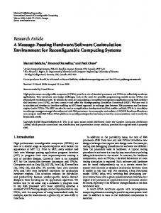
Abstract In recent years existing development methods have undergone a progressive advancement. Rising design complexity, the need to reduce time-to-market, and the integration of heterogeneous fields like electronics, mechanics, and software into a single product have been demanding a steadily enhancement of existing design environments, tools, and methods. Today simulation is a standard technology featured by almost every design process. Simulations incorporating different design stages of single parts of the system enable the validation of the design in respect of its specification during the entire design process, as well as the verification of single development steps. Therefore it is possible to detect design flaws, misinterpretations of interfaces and the results of error-prone design team communication like out-of-date specifications and poorly communicated model changes as early as possible. Heterogeneity of system descriptions poses a severe challenge to simulation. However distinctive features of single design languages, the availability of well tested design solutions, valuable experience of engineers in special languages and tools, or even the integration of foreign solutions may result in a heterogeneous system description. Simulators featuring multiple design languages and methods are scarcely available. Therefore simulator couplings try to provide solutions for the simulation of heterogeneous system through a combination of appropriate simulators via special interfaces. Similar interfaces enable the integration of real hardware or emulators into the simulation, to accomplish a simulation speedup. For the realization of a cosimulation various approaches are available, implementing single aspects like the synchronization of the single simulators in different ways. In this work a cosimulation environment for design processes using Simulink, Modelsim and SystemC is developed. To achieve a cosimulation, network connections are used to synchronize the single simulators data-driven and cycle-based.

2

Danksagung

Bedanken m¨ ochte ich mich bei jenen Mitarbeitern des Instituts f¨ ur Technische Informatik, die direkt oder indirekt zum Gelingen dieser Diplomarbeit beigetragen haben. Im Besonderen bei O.Univ.-Prof. Dr. Reinhold Weiss f¨ ur die Möglichkeit, diese Arbeit an diesem Institut durchf¨ uhren zu k¨ onnen und deren Begutachtung. Besonders hervorzuheben ist auch Ass.-Prof. Dr. Christian Steger, der mich bei der Durchf¨ uhrung dieser Arbeit betreut hat und durch seine Anregungen, Verbesserungen und Korrekturen einen sehr wertvollen Beitrag zu der vorliegenden Diplomarbeit geleistet hat. Mein Dank gilt auch Dr. Markus Pistauer, Managing Director der Firma CISC Semiconductor Design+Consulting, der in Kooperation mit dem Institut f¨ ur Technische Informatik diese Diplomarbeit erm¨ oglichte. Hervorzuheben sind hier auch seine Mitarbeiter Simone Reale und Dipl.-Ing. Suad Kajtazovic, die meine Arbeit mit ihren Vorschlägen und ihrem zur Verf¨ ugung gestellten Erfahrungsschatz bereichert haben. Dar¨ uberhinaus m¨ ochte ich mich bei meinen Eltern bedanken, die mir den Weg zum Studium geebnet und mich auf meinem ganzen bisherigen Weg unterst¨ utzend begleitet haben. Herzlichen Dank auch an meine Freunde, die meine Studienzeit berreichert und mich auch bei meiner Diplomarbeit durch Korrekturlesen und aufmunternde Gespräche unterst¨ utzt haben. Besonderer Dank gilt meiner Freundin Romana, deren Nerven ich in den letzten Jahren oft bis hart an die Grenzen strapaziert habe. Sie hat endlose Geduld mit mir bewiesen und mich auch in schlechten Zeiten nicht die schönen Dinge im Leben vergessen lassen.

Graz, im Oktober 2003

Ingo Hans Pill

3

Contents 1 Introduction and Motivation 9 1.1 Objectives . . . . . . . . . . . . . . . . . . . . . . . . . . . . . . . . . . . . . 12 1.2 Document Structure . . . . . . . . . . . . . . . . . . . . . . . . . . . . . . . 12 2 Background and Related Work 2.1 Design, Validation and Verification . . . . . . . . . 2.2 Verification and Validation via Testbenches . . . . 2.3 Heterogeneity in System Design . . . . . . . . . . . 2.3.1 Multiple Levels of Abstraction . . . . . . . 2.3.2 Inter-Domain Design . . . . . . . . . . . . . 2.3.3 Module Reuse and Integration of Foreign IP 2.4 Simulation of Heterogeneous Systems . . . . . . . . 2.4.1 Homogeneous Simulation . . . . . . . . . . 2.4.2 Heterogeneous Simulation . . . . . . . . . . 2.5 Simulators . . . . . . . . . . . . . . . . . . . . . . . 2.5.1 Models of Computation . . . . . . . . . . . 2.5.2 Simulator Connections . . . . . . . . . . . . 2.6 IP Core Business . . . . . . . . . . . . . . . . . . .

. . . . . . . . . . . . .

. . . . . . . . . . . . .

. . . . . . . . . . . . .

. . . . . . . . . . . . .

. . . . . . . . . . . . .

. . . . . . . . . . . . .

. . . . . . . . . . . . .

13 13 15 16 17 19 20 21 21 24 33 33 36 42

3 Design of the Cosimulation Environment 3.1 Development Profiles . . . . . . . . . . . . . . . . . . . . . . . . . 3.2 A brief Overview of Simulink, Modelsim, and SystemC . . . . . . 3.2.1 Simulink . . . . . . . . . . . . . . . . . . . . . . . . . . . . 3.2.2 Modelsim . . . . . . . . . . . . . . . . . . . . . . . . . . . 3.2.3 SystemC . . . . . . . . . . . . . . . . . . . . . . . . . . . . 3.3 Considerations for a Model of Computation for the Cosimulation 3.3.1 Time and Synchronization . . . . . . . . . . . . . . . . . . 3.3.2 Cosimulation Control and Communication . . . . . . . . . 3.4 The global cosimulation concept . . . . . . . . . . . . . . . . . . 3.5 Interfaces for Simulink, Modelsim and SystemC . . . . . . . . . . 3.5.1 MATLAB/Simulink . . . . . . . . . . . . . . . . . . . . .

. . . . . . . . . . .

. . . . . . . . . . .

. . . . . . . . . . .

. . . . . . . . . . .

. . . . . . . . . . .

. . . . . . . . . . .

45 45 46 46 49 51 53 53 56 58 60 60

4

. . . . . . . . . . . . . . . . . . . . cores . . . . . . . . . . . . . . . . . . . . . . . . . . . .

. . . . . . . . . . . . .

. . . . . . . . . . . . .

. . . . . . . . . . . . .

3.5.2 3.5.3

Modelsim . . . . . . . . . . . . . . . . . . . . . . . . . . . . . . . . . 64 SystemC . . . . . . . . . . . . . . . . . . . . . . . . . . . . . . . . . . 67

4 Implementation of the Cosimulation Environment 4.1 Communication Mechanisms using Sockets . . . . . . . . . . . . . 4.1.1 Stream Sockets . . . . . . . . . . . . . . . . . . . . . . . . 4.1.2 Programming Stream Sockets . . . . . . . . . . . . . . . . 4.1.3 Implementation of the Cosimulation Communication . . . 4.2 Simulink Interface . . . . . . . . . . . . . . . . . . . . . . . . . . 4.2.1 Real-Time Workshop Code Creation Process . . . . . . . 4.2.2 Simulink Wrapper Concept . . . . . . . . . . . . . . . . . 4.2.3 Simulink Wrapper Realization . . . . . . . . . . . . . . . . 4.3 Modelsim Interface . . . . . . . . . . . . . . . . . . . . . . . . . . 4.3.1 General Modelsim Wrapper Concept . . . . . . . . . . . . 4.3.2 Creation of a Foreign Architecture . . . . . . . . . . . . . 4.3.3 Modelsim Wrapper Realization . . . . . . . . . . . . . . . 4.3.4 Summarized Modelsim Wrapper Implementation Concept 4.4 A Wrapper for SystemC . . . . . . . . . . . . . . . . . . . . . . . 4.4.1 Building a SystemC Entity for a Foreign Module . . . . . 4.5 Cosimulation Setup and Results . . . . . . . . . . . . . . . . . . .

. . . . . . . . . . . . . . . .

. . . . . . . . . . . . . . . .

. . . . . . . . . . . . . . . .

. . . . . . . . . . . . . . . .

. . . . . . . . . . . . . . . .

. . . . . . . . . . . . . . . .

70 70 71 72 76 80 81 85 87 92 92 94 95 99 101 102 104

5 Conclusion and Perspectives

111

A List of Acronyms

113

B Examples 114 B.1 Example Stream Socket Server & Client . . . . . . . . . . . . . . . . . . . . 114 B.1.1 An example server program . . . . . . . . . . . . . . . . . . . . . . . 114 B.1.2 An example client program . . . . . . . . . . . . . . . . . . . . . . . 115 Bibliography

116

5

List of Figures 1.1

Abstraction vs. complexity during IC-design . . . . . . . . . . . . . . . . . . 10

2.1 2.2 2.3 2.4 2.5 2.6 2.7 2.8 2.9 2.10 2.11 2.12 2.13 2.14 2.15 2.16 2.17

The strategy of a testbench . . . . . . . . . . . . . . . . . . . . . . . . . . . Y-diagram according to Gajski and Kuhn . . . . . . . . . . . . . . . . . . . Module verification at different abstraction levels . . . . . . . . . . . . . . . Decomposition, modularization, and module reuse in a design process . . . Illustrating the expressible models for two languages: The general situation Illustrating the expressible models for two languages: A special case . . . . Introducing a third language . . . . . . . . . . . . . . . . . . . . . . . . . . A schematic principle of a backplane . . . . . . . . . . . . . . . . . . . . . . Three rule sets for a backplane protocol implementation. . . . . . . . . . . . Automated interface generation for a SystemC based backplane . . . . . . . A cosimulation of an optical cross connect using a SystemC backplane . . . A backplane communication interface for a VHDL model . . . . . . . . . . The entities of the introduced VHDL interface . . . . . . . . . . . . . . . . A hybrid system containing a discrete controller and a continuous plant . . An UML diagram for an object-oriented interface for Simulink models . . . The effect of simultaneous events in discrete event computational models . . Dataflow networks: (a) a directed graph (b) a corresponding single-processor static schedule . . . . . . . . . . . . . . . . . . . . . . . . . . . . . . . . . . 2.18 Backtracking within a simulation . . . . . . . . . . . . . . . . . . . . . . . . 2.19 Nested remote procedure calls . . . . . . . . . . . . . . . . . . . . . . . . . .

15 18 19 21 22 22 23 25 26 27 28 29 30 31 32 34

3.1 3.2 3.3 3.4

A typical hardware design flow: a) standard and b) with SystemC Cosimulation synchronization illustration . . . . . . . . . . . . . . General cosimulation concept . . . . . . . . . . . . . . . . . . . . . Real-Time Workshop rapid prototyping execution flow chart . . . .

. . . .

. . . .

. . . .

. . . .

. . . .

53 58 59 64

4.1 4.2 4.3 4.4 4.5

Problematic connection establishment sequences Real-Time Workshop code creation process . . . A simple Simulink model . . . . . . . . . . . . . Simulink simulation parameters tablet . . . . . . Real-Time Workshop parameters. . . . . . . . . .

. . . . .

. . . . .

. . . . .

. . . . .

. . . . .

77 81 82 83 83

6

. . . . .

. . . . .

. . . . .

. . . . .

. . . . .

. . . . .

. . . . .

. . . . .

. . . . .

. . . . .

36 37 40

4.6 4.7 4.8 4.9 4.10 4.11 4.12 4.13

Real-Time Workshop target selection. . . . . . . . . . . . . . . . . . . . . . 84 Simulation concept of the Simulink wrapper . . . . . . . . . . . . . . . . . . 87 Integration of the Modelsim wrapper into a VHDL simulation . . . . . . . . 93 An example system based on an ASIC and a test-bench . . . . . . . . . . . 104 Time-diagram of signal ”A” determined at a Simulink simulation . . . . . . 108 Time-diagram of signal ”A” determined at a Simulink cosimulation . . . . . 109 Time-diagram of signal ”A” determined at a Simulink - Modelsim cosimulation109 Time-diagram of signal ”A” determined at a SystemC based Simulink cosimulation . . . . . . . . . . . . . . . . . . . . . . . . . . . . . . . . . . . . . . . 110

7

List of Tables 3.1

Features supported by several Real-Time Workshop targets . . . . . . . . . 48

8

Chapter 1

Introduction and Motivation In recent years existing development methods have undergone a progressive advancement. Rising design complexity, the need to reduce time-to-market, the integration of heterogeneous fields like electronics, mechanics, and software into a single product, or the evolvement of SOC1 -designs have been demanding a steadily enhancement of the entire design process; additionally all involved environments, tools, and methods had to be improved too. As an example for interdomain design the development of a car can be taken, which encompasses the development of mechanical and electronic parts as well as some control software, not to forget the aerodynamics of the coachwork. An ideal design process should enable the possibility to work in all these areas concurrently to minimize time-to-market, as well as the facility to perform integral tests of the entire product at every design stage. To cope with this request of first magnitude new industry branches specialized in interdomain-design, like Mechatronic, have occurred in the industrial landscape, as application areas for inter-domain design could be found in almost every product used in everyday life. Heterogeneity in a system design is not only a reason of the product area, but for example may also result from different design environments used throughout the development process. To reduce time-to-market and therefore reduce costs for instance, it is necessary to divide the problem or task or product into several parts to be conquered by multiple design teams. Using this divide-and-conquer principle makes it necessary to validate complete system interaction throughout the entire design process. Due to this it is possible to detect design flaws, misinterpretations of interfaces, and the results of error-prone design team communication, like out-of-date specifications and poorly communicated model changes, as early as possible. 1

System On a Chip

9

10

CHAPTER 1. INTRODUCTION AND MOTIVATION

These validation and verification steps might be faced with a heterogeneous system. This can result from the use of several specialized tools for the different system parts, or the verification of parts in different design phases. A common example for the verification of modules at different design phases and detail levels would be the verification of an algorithmic description of a test module in combination with a transistor representation of an IC2 . The prior mentioned design phases represent an approach to deal with the increasing complexity of systems. Several levels of abstraction are introduced, in a way that different aspects of model design are dealt with at different stages of the design process. For example a product’s functional design is done at an early stage without dealing with implementation problems at transistor level or even thinking about C-MOS3 process technologies. Figure 1.1 shows the typical abstraction levels (or layers) found in an IC design process and their responding detail levels illustrated by the amount of components (design elements) the designers are faced.

System

1E0 1E2

RTL

1E3 1E4

Gate

1E5

Transistor

1E6

Abstraction

1E1 Algorithm

Complexity, Accuracy

Level of Abstraction

1E7

Complexity − Number of Components Figure 1.1: Abstraction vs. complexity during IC-design [DG00]

As a consequence of the prior mentioned divide-and-conquer principle, the utilized partitioning and modularization processes have evolved in a way that the reuse of single modules became possible. Figure 2.4 at page 21 illustrates this concept. Such a module reuse may be considered to be either within the design itself, or in a way that standard cells shall be designed which may then be reused in other products as well. The creation of libraries containing standard modules, as well as the development of design environments 2 3

Integrated Circuit Complementary Metal Oxide Semiconductor


11

supporting the concept of model reuse have been gaining such importance that a new business branch called IP-Core4 business has emerged. IP-Core business demands technical solutions to provide such libraries to customers without publishing the intellectual property itself, but with a maximum usability and interconnectivity to a customer’s design. After considering the above mentioned general aspects and problems of a design process, they shall be reconsidered with a practical aspect of product design in mind: simulation. Today simulation is one of the major concepts of design environments. Simulation is used to verify the different steps made during a design process and therefore is a major tool to ensure that a design lives up to the product requirements. Simulating a design beginning at the very first development stage and abstraction layer offers the ability to show the behavior and reveal errors or design flaws as early as possible. Also when transitioning from one level of abstraction to a deeper one during a design process, a cosimulation of single modules at the deeper level with the rest of the system represented in the already verified higher level is a powerful method to verify those level transitions. Inter-domain co-simulation would be a desired tool in a design process as well. Simulation has many other advantages such as minimizing the need of prototypes, or the fact that in several areas like nuclear and other elementary research areas development of products would be much more time-consuming and expensive or sometimes even impossible. Summarizing, design environments and tools had and still have to be developed which make it possible to provide concise models of systems with multiple domains and at different abstraction layers in conjunction with methods to ”test” the design at every design stage [PKPS03]. Single component simulation should be featured as well as the simulation of the entire system, at every single and between different levels of detail. Furthermore the tools should support module-reuse as well as the integration of foreign modules and designs. These requirements are quite challenging and there exist numerous different approaches, methods and tools trying to cope with at least parts of these expectations.

This task also represents the motivation for this diploma thesis. The aim of the thesis is to develop a methodology for a heterogeneous cosimulation of different modules designed with MATLAB/Simulink, Modelsim(VHDL), and SystemC. These design tools and environments have distinctive features, aim on different detail levels, and are commonly used in the development of systems using electronic and mechanical parts. The above discussed aspects of design environments will be considered during the design of this cosimulation methodology to offer an efficient, feature rich, and thus powerful approach. 4

Intellectual Property Core


1.1

12

Objectives

MATLAB/Simulink, Modelsim(VHDL) and SystemC are powerful tools utilizing different languages offering their distinctive features and application areas. The aim of this work is to investigate methods to combine their power by providing a cosimulation method for these tools. This masters thesis results of a joint venture of the Institute for Technical Informatics at the Technical University Graz, and CISC Semiconductor Design+Consulting, Klagenfurt. At the beginning of this project the following topics were considered to be investigated in detail: • Exploration of generated C-code from the Simulink Real-Time Workshop for the possibility to be included into a VHDL simulation. • Simulation of a system containing components designed with Simulink and VHDL, using above mentioned C-code generation. • Investigation of the possibility to include this simulation into a SystemC simulation. For a verification of the developed methodologies a typical automotive or telecommunication application shall be used to ensure usability in industry.

1.2

Document Structure

The structure of this document is straight forward. The document starts with a short introduction discussing the motivation and objectives of this masters thesis. The introduction is followed by a chapter discussing the background basics considering different design and simulation aspects, and briefing several state of the art implementations and approaches. Afterward a simulation network will be designed in accordance to the desired project objectives, whose implementation is then presented in the implementation chapter. The document is completed by a discussion of the approach.

Chapter 2

Background and Related Work In recent years existing development methods have undergone a progressive advancement. Design processes and tools have been enchanced in many ways to handle rising design complexity and inter-domain designs as well as to minimize time-to-market. In this section several aspects of design processes will be discussed to provide the basics for the design of a heterogeneous cosimulation scheme. Furthermore related work will be addressed and projects implementing the mentioned technologies presented.

2.1

Design, Validation and Verification

Design processes may differ in many aspects from each other; in respect of the used strategies like bottom-up or top-down approaches (as illustrated on page 18), or special used techniques like extreme programming [Bec99], used tools, or simply organizational aspects. Despite this diversity, there is one common requirement present with every single design process; The need to validate the design and to ensure the consistency of accomplished work during single development steps. This includes validation of an initial specification, the verification of a single decision made done during a development process, as well as the ”real world” testing of the result at the end. In literature different distinctive terms for these ”testing” steps have emerged [Zim03]: • Validation is used to answer the key question whether a product will live up to the expectations. This starts with a validation of the specification and may be done throughout the complete development process. • Verification considers design steps. Verication steps are intended to ensure a design’s consistency during one or more actions carried out within a design process. There may be small changes in a design, but the requirements always have to be met. Therefore verification has a tight relationship to validation. Verification may consider the entire system or single parts of it. 13

CHAPTER 2. BACKGROUND AND RELATED WORK

14

• Testing is done when the development process is completed and the product is ready for production. Therefore it is intended to unveil errors in the production process and is furthermore a means of quality assurance. Summarized ”validation” and ”verification” are used to unveil errors and flaws during a design process. Afterward prototypes are ”tested” to detect production errors. Although the intentions aim on different aspects, in practice the steps carried out may not be dedicated precisely, as these tasks are tightly bound by their intention. For illustration consider the following: Testbenches may be used for both verification and validation. Semantically testbenches are a means of validation, as testbenches try to answer ”does it fulfill the expectations?”. Comparing testbench results before and after a design step is a means of verification, as the intention is to investigate design consistency over a design step. Furthermore there may still be design errors and flaws in the finished design, just uncovered at the testing of the ready-to-market product. There exist formal techniques like equivalence-checking or model-checking for validation and verification [Zim03, ELESV97]. However these formal methods are very hard to perform especially with increasing complexity, and depend on special description formalisms, constructs and languages to be used within model descriptions. In contrary to formal approaches, there exist several practical approaches as well, which utilize the idea of testbenches and will be discussed in more detail on page 15. These practical approaches like simulation and emulation have however a severe drawback which is caused by its internal strategy. These methods implement testbenches, whereas the considered item is fed with distinctive inputs to observe the output. The output will then be interpreted to determine whether the item operates as intended. The problem with this scheme is, that it does not fully live up to the expectation of providing a general correct testimony whether the item is operating correct or not, but the conclusion is only correct for the used test scenarios. A consideration of a typical state-of-the-art microprocessor like AMD’s Athlon 64 shall unveil the arising problem. A single 64 bit addition would result in 2128 different input combinations to be considered. With a given simulation time of one microsecond per input combination, it would still take about 1025 years to consider every single possible input combination. Taken the complexity of the entire processor with all its units and states, it becomes even more obvious that testing the entire processor with all its possible input combinations and states to detect side effects is absolutely infeasible. So engineers have to construct test cases covering as many eventualities as possible. However they are not able to ensure testing every single eventuality using testbenches. Providing correct methods for verification and validation is a difficult task, as is even the establishment of a ”high quality specification” to rely on. There exist many more aspects to consider with both formal and testbench methods, however only a short introduction is intended to be given at this point. As the testbench

15


approach will be featured within this work as it perfectly refers to a cosimulation approach it will be discussed in regard of practical aspects in the next section.

2.2

Verification and Validation via Testbenches

Szenarios

DUT

Output Data

possible

Input Data

As mentioned in the prior section, the strategy of using testbenches serves to consider a system’s behavior. The considered target receives well considered input scenarios (test cases), whereas its reaction to this stimuli is evaluated to predict the target’s behavior. Figure 2.1 illustrates this behavior.

Evaluation Feedback DUT .... Device Under Test

Figure 2.1: The strategy of a testbench: Possible scenarios provide the input data for a DUT. The output data can be evaluated for validation purposes and might influence the next input data set Methods to determine system behavior within a testbench include entire software solutions and approaches utilizing at least the (partial) inclusion of hardware for gaining a speedup [Zim03, Rei98]. Simulation is an approach completely based on software, with all pros and cons entailed. So if a simulator is available for the used system description formalism, a simulation can be performed with a minimum of overhead and costs. Parameters like granularity of the results or time resolution can be changed easily. This enables a very flexible reconsideration of single design steps, and simple design errors can be easily managed by iterative simulation and model alteration cycles. In dangerous application areas like nuclear power plants or other areas where testing prototypes could cause severe damage, simulation is a mandatory technology. There exist many advantages with simulation due to its flexibility, minimized costs and wide application area. However there are several drawbacks as well. First of all a successful simulation is no guarantee for the functionality of a product. Besides of the impact of limited test cases as discussed in the prior section (page 14), a simulator is a piece of software which is (in most cases) not formal proven and may contain errors. In practice simulators are not very flexible, as in most cases they implement one single language with limited expressiveness featuring only a subset of possible designs. Simulator internal interfaces for interconnection with third party software and


16

other simulators to enhance the amount of possible designs are limited and proprietary if even present. Last but not least simulation becomes very slow with increasing complexity of a system, as the calculation time rises as well as the minimum amount of test scenarios needed for a valid behavior assumption. Emulation is one of the possible solutions for this problem. During the design of an IC1 for instance FPGA2 s and automatic synthesis tools may be used to map the description of a design onto hardware to create a virtual chip. This virtual chip may then be connected to the actual testbench. Although the speed of this chip might be much slower than the finished product, it will be still much faster than simulation. A drawback to emulation are its high costs, as well as the fact that the hardware would have to be replaced quite frequently, due to the fast increasing complexity. [Rei98] uses real hardware integrated into a simulator for a speed-up. So real parts of the system, for instance an already developed IC, may be integrated into a simulation as well. Methods of the inclusion of existing hardware into a simulation or emulation offer further advantages as well, as it could be possible to test a design in real world conditions. For example a control IC can be tested in its application of controlling some mechanical part. Although possible the inclusion of real hardware into a simulation is in practice limited by the technology available today as for instance real-time simulation would be mandatory for interactive real world situations. For much simpler situations like integrating a real IC into a VHDL Simulation there exist already solutions as can be found in [Zim03, Rei98].

2.3

Heterogeneity in System Design

Heterogeneity is a plurivalent word in respect to a design process, although the classification into homogeneous and heterogeneous systems is very common in system design. This separation is not really that explicit, as the decision whether a system is heterogeneous or homogeneous, can be based on many different special aspects of the considered system. For instance if a system consists of multiple subsystems related to different domains (e.g. software and hardware) it is heterogeneous in respect of its domain. However it may be homogeneous in respect to its description language, if all system parts are modeled in the same language. As this classification is ambiguous, for this document ”heterogeneity” shall refer to the latter mentioned aspect if not mentioned otherwise; to the description language(s) used for system representation. A homogeneous model is therefore modeled in one single language, 1 2

Integrated Circuit Field Programmable Gate-Array


17

whereas a heterogeneous model utilizes multiple language sets. It is a very difficult task to cope with heterogeneity and it entails some severe problems for the design process. Especially in respect to validation and verification it is a considerable obstacle due to the limitations of single simulators. Therefore cosimulation technologies have to be used for a simulation of the entire system. However there exist severe reasons for the demand and existence of heterogeneous system models. The following three situations will be discussed in detail in the very next subchapters: • Multiple levels of abstraction • Different domains • Module reuse or the integration of foreign IP-cores3 Although these situations seem to be very different to each other, they can be assigned to two main origins. The limitations encountered with the use of a single description language and the reuse of available models or know-how. The first basic origin results from the lack of a general description language as discussed in [Sim98]. For a special project the limitations of a single language in respect to its basis elements, description concepts, or paradigms may require either the enhancement of this language to support special needs, or the partitioning of a system, so that each part can be modeled in an appropriate language. Available know-how and standard modules, or the integration of foreign designs may result in heterogeneous system designs as well. There exist multiple different languages and tools with their own distinctive features and application areas. Besides language abilities themselves, the experience of engineers with their tools shall be considered as well, as this experience minimizes design times and results in a better quality as well. The reuse of already available ”well tested” modules is a considerable option too, independent of the source of the module description. It may come from standard libraries, former projects, or even bought foreign designs. In many cases these will not be available in the actual used description language, and in the case of foreign designs they may further be encapsulated in a special format to hide detail informations and intellectual property.

2.3.1

Multiple Levels of Abstraction

Abstraction layers or levels have been introduced to cope with the increasing complexity of products to be developed. The intention was to consider different aspects of a system at different stages. Figure 2.2 at page 18 illustrates the typical abstraction levels used for electronic circuit design processes. 3

Intellectual Property cores

18

CHAPTER 2. BACKGROUND AND RELATED WORK System Level Algorithmic Level

Behavioural

Structural

Register−Transfer Level System−Specification

CPUs, Memory

Logic Level

Algorithms Register−Transfers

Subsystems, Busses Modules, Registers, ALU

Circuit Level

Boolean Equations

Flip−Flops, Gates

Differential Equations

Transistors

Production Masks , Polygons

Cells

Floorplan

Cluster

Partitioning

Physical/Geometry

Figure 2.2: Y-diagram according to Gajski and Kuhn, adapted from [LWS94] In this figure the abstraction levels are represented by circles, the minor the radius the greater the level of detail, whereas the three axes are related to different point of views. Intersections of circles and lines represent modeling stages, where a designer may decompose a model (figure 2.4 on page 21). For system design the engineer will start at the outer region (system level) and then will head by transformations (change point of view) and refinements (change abstraction levels) to the center, what means he has an accurate model of the final implementation. Figure 1.1 at page 10 shows the complexity of the design process in respect of the amount of design elements the development teams are faced, and the accuracy represented by the abstraction level. A typical top-down design methodology starts with a specification at the highest level of abstraction, the so-called system level, and moves step-wise down to more detailed levels by refining and decomposing the model (see fig. 2.4 at page 21). In most cases a design won’t utilize a simple top-down approach, because verification between different abstraction levels will unveil errors and design flaws and as a consequence the model has to be modified or even redesigned (maybe at a higher level of detail). The resulting methodology is referred as ”jojo”-design. Bottom-up methodologies work the opposite way, they start at the lowest detail level and proceed by composing components together. These component blocks may be used

19


in the next step to create even more complex components. The creation of standard cell libraries is a certain strength of this approach. The verification between different abstraction levels is one of the key-issues for the entire design process. During refinement steps between detail levels, or decomposing phases at one level, the model’s invariance to the specification has to be monitored and guaranteed. To accomplish this, the interaction of multiple modules at different abstraction levels has to be validated, as illustrated in figure 2.3 where module 3’s invariance is tested.

M1

M2

M3

M4

System−Level

Simulation

Verification

M3_c System−L. M1

M2

M3_b Gate−L.

System−Level

M4 System−L.

M3_a Reg.−Tr.−L.

Figure 2.3: Module verification at different abstraction levels As indicated in the figure, different languages may be used at different abstraction levels. This illustrates the need of cosimulation methods for several simulators to enable the verification steps utilizing different abstraction levels [PKPS03].

2.3.2

Inter-Domain Design

Inter-domain design is a matter of first magnitude. Today a common system design may include components from heterogeneous fields like electronics, mechanics, software, and many more e.g. [IEE99]. To be able to detect errors and side-effects of possible changes as soon as possible, validation and verification of the entire system throughout the whole design process is mandatory. For convenience there has always been the wish for one universal language able to describe everything and understandable by every tool. Besides the theoretical question of whether such a language does even exist, today’s tools aren’t able to live up to these expectations. Although languages have been enhanced to offer functionality for at least similar domains, this enhancements entailed drawbacks as well.


20

To create a precise and accurate description of a model related to special domain, the used language has to offer special constructs and components representing the distinctive features of this domain. If a language tries to cover multiple domains, it provides this interdomain functionality at expense of flexibility and modeling power in the single domains. Considering multiple domains in combination with different layers of abstraction unveils the amount of functionality a single language would have to provide. Even if there exists a language to cover all domains of a system, there may be a reason to use multiple ones. Engineers related to a special domain in most cases rely on special tools providing best functionality in this domain, and have a deep know-how and experience with their tools of choice. For a homogeneous system description all engineers would have to abandon their know-how and learn a new tool covering all aspects of this single system. Furthermore this ”general language” might be different for every single product. As there is an enormous amount of different domain-combinations, all covered by different languages dependent on the specific system’s requirements, it would be a very inefficient and time-consuming alternative to switch description language every time to get a homogeneous system description. Again for verification and validation purposes cosimulation methods have to be provided [PKPS03].

2.3.3

Module Reuse and Integration of Foreign IP cores

”Modularization” and ”Reuse of Modules” (illustrated in fig.2.4) are two essential key principles of state-of-the-art design processes. They enable short design times and minimize origins of error due to the reuse of well-tested components. The aim of modularization is to divide a huge complex system into several subsystems easier to cope with, what can be done repeatedly in a design process. Through intelligent partitioning some components may be reused within the model itself, or already completed models from earlier designs may be integrated. The creation of a standard-component library should be an option considered during the partitioning steps as well. Figure 2.4 illustrates this concept of decomposing and reuse. This principle has formed a completely new branch of (semiconductor-)industry: the ”IP 4 Core Business” [GWC+ 00]. In this business IP core providers offer their know-how and developed models packaged in IP cores. A company might buy these cores for integration into their own design, instead of developing everything on their own. This integration process has different obstacles to conquer, as the IP provider may use a special distribution format for enclosing the IP itself, or at least uses other languages (for all or single abstraction levels). Therefore module reuse and especially the integration of foreign parts may lead to a heterogeneous design situation. A more detailed discussion of IP core business can be found in section 2.6 at page 42. 4

Intellectual Property

21


System 1

System 2 Decomposition

Level 1

Refinement Decomposition

Level 2

Refinement Already

Level 3

Dec.

Developped

Model Reuse

Figure 2.4: Decomposition, modularization, and module reuse in a design process

2.4

Simulation of Heterogeneous Systems

Today there exists a steadily increasing amount of different design and simulation tools, whereas single tools have reached importance in specific domains or for special purposes. As discussed in the prior section this fact is one of the reasons for heterogeneous system descriptions. Heterogeneous system descriptions pose a challenge for an engineer in respect of its validation and verification. Simulation is one of the means to predict the behavior of a system for validation against its specification, or to verify special design steps. However there hardly exist simulators featuring multiple languages and description concepts. In this section methods will be discussed to perform a simulation of a system represented by a heterogeneous description. To accomplish this there exist homogeneous and heterogeneous approaches, implying the fact that a heterogeneous design does not automatically implicate the need for heterogeneous simulation, as there exist approaches to transform heterogeneous models into homogeneous ones.

2.4.1

Homogeneous Simulation

The distinctive feature of all homogeneous simulations is that they utilize only one single simulator for system evaluation. Every simulator has its own distinctive special instruction and construction set for control and model description. Thus a system to be simulated by this simulator has either to be designed with these


22

distinctive sets, or a heterogeneous system description has to be transformed into a homogeneous model compatible to this simulator. The transformation of a heterogeneous model into a homogeneous one contains some kind of translation. Consider a model using two different languages, possible strategies could be: • The translation of modules described in language A into language B which is used for the rest of the system. • The introduction of a third language accompanied by the translation of all modules into language C. Although the latter approach might sound more complicated, because of the involvement of a third language C, the following figures show the reason why it might be the only possibility to obtain a homogeneous system model. Considering the instruction set of a single language A and the set of modules which may be described by it (L1) compared to that of another one (L2) unveils the major problem with translation methods due to language boundaries(fig. 2.5). Only the intersection of both (L1+L2) contains models which may be described in either language and thus may be translated from one into the other. L1

L1 + L2 L2

Figure 2.5: Illustrating the expressible models for two languages: The general situation Possible variation of this intersection according to mathematical ”Theory of Sets” shows specific situations, where the complete set of modules from one language might be translated into the other one. In practice these situations will be very rare, as it is only possible if one language (e.g. L1) is a subset of or equal to the other one (e.g. L2), as illustrated in figure 2.6.

L1

L2

Figure 2.6: Illustrating the expressible models for two languages: A special case, where L1 is a subset of L2


23

The introduction of a third language changes the situation to some extent due to the introduction of new dependencies. Figure 2.7 shows two different intersection sets to illustrate these new variants. L2

L1

L2 L1 L3

L3

Figure 2.7: Introducing a third language: (a) left: general case (b) right: L1,L2 are a subset of L3 Considering figure 2.7 it is obvious that a possible homogeneous simulation of modules of language A (L1) and language B (L2) is partly independent on the relation between their languages. The introduced language offers new possibilities due to its own relations. Case (a) of figure 2.7 shows a general case where only subsets of L1 and L2 can be translated into language C (model set L3), whereas case (b) shows an extrema where L1 and L2 are a subset of L3 and thus all modules L1 and L2 may be translated into language C. In both cases a homogeneous model is achievable (in case a only for subsets) although the original languages L1 and L2 are incompatible to each other. An illustration for this, not related to simulations, is the compilation of a heterogeneous programs to obtain an executable. For instance when designing a program for e.g. a 80535 micro controller containing C-parts as well as assembly routines, both language domains get assembled and compiled into an intermediate language understandable by a linker which merges the different object models to obtain the desired executable. Considering language sets and subsets only covers theoretical solutions regarding language compatibility by determining their boundaries. In practice there is neither a standard for the documentation of these sets, nor is it usual to specify them in a languages’ documentation. The exact determination of the sets is a very hard task, as is the mapping of a set of real systems to a set of system models. To implement this approach vague determinations of these sets will be made. Although this example of compiling a program is not related to simulation, the process of the translation within a standard computer compiler is the same which will be used to achieve a homogeneous system description. It will include the analysis of the description in several aspects (syntax, semantics) and the actual code creation process. The construction of such compilers is a non-trivial task illustrated in the ”Dragon-book” [ARJ99a, ARJ99b]. There exist several projects related to simulation implementing the approach of creating a homogeneous system description: • In [bib97] translation is used for a cosimulation of Statemate and SDL5 models. A 5

Specification and Description Language


24

subset of statechart may be translated into SDL. • The ”European SystemC User Group” provides a VHDL to SystemC converter. With the VHDL-to-SystemC converter you can transform VHDL hardware descriptions into SystemC hardware descriptions. The converter supports only subsets of VHDL and SystemC, so not every VHDL description could be converted. The tool is available for SUN Solaris and PC Linux workstations and includes two short examples. It is available at [Eur]. • University of Verona, Italy provides in [Unia] detailed information on version 1.0 of their VHDL to SystemC converter ”VHDL2SC”, containing the translation rule set. This tool is based on SAVANT [Exp] and adds the ability to translate the IIR6 format generated by SAVANT into SystemC code.

2.4.2

Heterogeneous Simulation

The counterparts to homogeneous approaches are heterogeneous simulations, utilizing more than one simulator for system simulation. Simulator interaction and couplings form the basis for this approach. Regarding the interaction scheme between the single parts of such a simulation network there are two major implementation strategies: • Backplanes • Direct Couplings The criteria for a classification to these strategies is the way different simulators communicate with each other. Backplanes use a central entity connected to every simulator, which has control to the whole simulation. Therefore simulator interaction operates indirect via the backplane. The other branch of heterogeneous simulation approaches uses specialized direct simulator-connections. Both options are discussed in the following: Backplane Approach As mentioned before backplane approaches utilize a central control unit, connected to each simulator, to manage the simulation. A backplane introduces a common simulator interface which has to be implemented with all simulators, so that all different simulators may be accessed via a special API7 . This API provides the necessary mechanisms for data communication and synchronization. A backplane takes control of all connected simulators (see fig. 2.8). To be able to integrate a special simulator into a backplane environment, there has to be a special wrapper for this specific simulator translating common API commands and data types into the specific simulator’s command-set as seen in figure 2.8. 6 7

Internal Intermediate Representation [Unib] Application Programming Interface


25

System model electronics part 1

mechanics part 2

software part 3

Sim. 1

Sim. 2

Sim. 3

Wrapper 1

Wrapper 2

Wrapper 3

simulation backplane (synchronization / data exchange)

User

Figure 2.8: A schematic principle of a backplane The presence of a common API to all simulators is a key feature of backplane environments and offers multiple advantages: • Easy integration of a new simulator into the simulation environment, especially if there already is a wrapper which may be reused. • Abstraction of simulators: Communication between simulator and backplane is simulator-independent which means data transfer and control are standardized actions. • For a possible speedup modules may be parted into several submodules which are distributed to multiple instances of a simulator. The integration of multiple instances of a simulator is very easy due to the reuse of the wrappers. A correct wrapper implementation is essential to a backplane environment. A function call of a backplane may result in different actions with different simulators. The actual wrapper translates this general backplane command to the specific simulator’s syntax. Data type and time format conversion is another task of the wrapper, as each simulator features distinctive internal formats. Thus a wrapper has to follow strictly the protocol of a backplane, which is essential to each backplane representing its distinctive features. A backplane’s protocol may be considered as the combination of three rule-sets [Bar99]. • Communication-rules describe the connection-handling between the backplanes and simulators, whereas the backplanes act as master and are therefore responsible for


26

connection establishment as well as sustaining and disconnection mechanisms. Data transfer control during simulation is necessary to enable correct ordering of simulator interconnection communication. • Synchronization-rules are used for the synchronization of the different modules. Interconnections between models require mechanisms for data-communication at these connections to provide data validity and avoid deadlocks. • Implementation-rules describe the implementation of the wrappers, and may be seen as translation scheme between the common-API commands and the unique and distinctive simulator command-sets. Synchronisation−rules Sim. 1

Sim. 2 Communication rules

Wrapper 1

Wrapper 2

Implementation−rules

simulation backplane

Figure 2.9: A backplane protocol consists of three rule sets: Implementation-rules, communication rules, and synchronization rules Most backplanes as well as their interfaces are implemented proprietary according to their specific intentions. However there are intentions to develop a standard for backplanes. The ”CAD Framework Initiative” (CFI) was founded in 1998 as a non-profit organization. It’s aim is to establish standards for the integration of CAD tools to enable design-data management as well as tool interoperability and a common user interface. Development was divided into several sub-projects including: • Design Representation Standard • Data Management • Inter-Tool Communication Standard • Tool Encapsulation Specification • Computing Environment Services Standard • Multi-Simulator Backplane


27

Interesting at this point is the CFI backplane standard. This standard defines the interface between different simulators and a backplane itself. It doesn’t represent an implementation of a specific backplane, but a general interface between an arbitrary simulator and an arbitrary backplane. This standard defines the partitioning of a system, common communication-rules, synchronization-rules, implementation-rules, and backplane operation as well as initialization at an abstract level intended for a general backplane description. A detailed discussion may be found in [Sim98]. There are many implementations of backplanes available, two of them briefed at this point for further illustration: In [NMK+ 02, KWG+ 02] a SystemC based backplane is used for the simulation and global validation of micro-electro-mechanical systems, whereas a free-space optical crossconnect using mirrors actuated by electrostatic devices is the actual DUT 8 . The control subsystem of this device was implemented in SystemC, the electro-mechanical part in MATLAB and the behavior of the optical devices (mirrors, lens, beam generators and detectors) in C++. In this approach hierarchical network lists of modules are used for system descriptions. Each module consists of a behavior and ports. These ports may be connected via communication channels. As the modules use different languages the implementation details differ from module to module. Wrappers are used to implement the general mechanisms for each module. They constitute the interfaces of the modules and isolate their internal behavior. Internal ports are connected to the module and external ports connect the module via channels to the global simulation. For convenience an automated generation of this communication and simulation interfaces is featured, based on internal libraries and specification of the module’s behavior and ports. Figure 2.10, illustrates this process and shows the resulting schemata of a cosimulation utilizing this approach.

Figure 2.10: A SystemC based cosimulation backplane with automated interface generation [KWG+ 02] 8

Device Under Test


28

To gain confidence of the desired approach a cosimulation of the mentioned optical cross-connect was performed to test the abilities of this system. The actual representation of this example is illustrated in figure 2.11:

Figure 2.11: Cosimulation of an optical cross connect using a SystemC backplane [NMK+ 02] The overall system simulation was performed on a SUN Ultra-Sparc 1 in about 30 seconds, and resulted in a successful test of the design and the cosimulation environment used for this test. where a SystemC based backplane is used for multi-domain and multilanguage cosimulation.


29

In [Bar99] Tvrtko Barbarić discusses HW/SW codesign based on a backplane approach. The developed cosimulation environment consists of the following three parts: • Backplane program • Interface-Link modules • Client-Simulators The implementations of these parts are based on a predefined backplane rule-set as illustrated on page 25. The backplane features event-driven scheduling with an event queue ordering future events. All data transfer between processes is relayed at the backplane to act as a global event queue. The backplane’s scheduler manages this queue and transfers events according to their global order, waiting for the response after each transfer. A general VHDL simulator interface for this backplane (as illustrated in figure 2.12) is introduced to achieve a hardware software cosimulation.

Figure 2.12: A backplane communication interface for a VHDL model [Bar99] Access to the VHDL model is based on several receive and send nodes and the use of a foreign architecture as shown in figure 2.13 at page 30. Foreign architectures are a special feature of the involved VHDL simulator offering the option to integrate foreign C-code into the simulation. The master node avoids deadlocks and controls the data transfers via sending and receiving special commands to and from the backplane. For a conclusion the used conservative timed synchronization strategy is discussed in respect of several optimization possibilities.


30

Figure 2.13: The different entities of the introduced VHDL interface [Bar99] Direct Couplings vs. Backplanes Contrary to backplanes many approaches for a heterogeneous cosimulation are based on direct simulator couplings. The main difference is the absence of a central control entity as featured with backplanes. With direct coupling two simulators are connected without considering interfaces to other simulators or interface standards. This includes minimal interfaces dealing only with special needs for a single project. The obvious advantage of direct couplings is that they range from minimal project specific approaches to general solutions for a powerful general purpose simulator interconnection. The origin and strategy of these approaches is very intuitive: If a simulator is not able to perform all tasks a designer needs it to, it has to be enhanced. A simple approach would be to enhance this simulator with special methods to integrate further functionality/resources by connecting a second simulator. An example would be the integration of a MATLAB Engine for mathematical computation as proposed in [Thea]. The use of a backplane would always inhibit the design of a complete interface regarding to the standards and protocols of the backplane, which is time-consuming A direct coupling would only need the implementation of features needed, and is even more flexible, as backplanes show limitations due to their used concepts and protocols. A major drawback of such a dedicated interface is its reusability as it is limited in sensitivity to the implementation strategy. A layered approach using standard functionality as found with backplanes would enhance it significantly. The most contrary feature of direct couplings versus backplane approaches is the lack of a central control unit. The operation of the complete environment, including synchronization and data management, is up to the simulators themselves and implied by the interface


31

implementation. A more detailed discussion of backplanes versus direct connections can be found in [Sim98]. In [Tud00] a dedicated direct simulator connection is used for a hybrid cosimulation. Signal and Simulink are used to model hybrid systems. Signal is a powerful tool for modeling complex discrete behaviors and Simulink is used to describe continuous dynamics. The combination of both is utilized to offer a cosimulation of a discrete controller controlling a continuous environment represented by a plant, as illustrated in figure 2.14.

Figure 2.14: A hybrid system containing a discrete controller and a continuous plant [Tud00] Two approaches to perform the desired cosimulation are presented in this work, whereas both make use of the ability of both tools to create stand-alone simulation code. In the first one, the system part modeled with Signal is the master and controls the changes in the continuous part, by using Simulink procedure calls. In the second approach the code created from the Simulink model is the master and the link between the discrete and continuous parts is implemented via global variables. The second approach is used to simulate the prior mentioned hybrid system. The Simulink main file runs the model simulation in an infinite loop illustrated by the following pseudo-code: while (true){ OneStep_Simulink_model; } After the calculation of one step, the simulation advances by a single time-unit. To synchronize the Simulink and Signal simulation this loop was altered by the author to include synchronous or asynchronous events of parts modeled in Signal:


32

while (true){ OneStep_Simulink_model; synchronous : OneStep_Signal_controller; asynchronous : if "triggered" then OneStep_Signal_controller; }

Data transfer is achieved via global variables as mentioned before. For a practical testing the approach was used to perform a cosimulation of a siphon pump machine. The availability of stand-alone code of the simulation provides great flexibility in respect of interconnectivity, as no proprietary interface of a simulator has to be used for an interface implementation but there might be the possibility to gain access to the simulation kernel and its environment The ability of Simulink to create stand-alone code of a simulation was used by another project as well, for the implementation of an object oriented interface [Mad00]. This interface may be used for direct simulator connections as well as backplane approaches. LaSRS++ is an object-oriented framework used by the NASA to create real-time simulations. As many simulation customers of NASA Langley Research center have selected MathWorks Simulink for their designs, the simulation software group at Langley created a reusable, object-oriented interface to integrate Simulink simulation code, provided via its Real Time Workshop, into the Langley Standard Real-Time Simulation. For the realization of an object-oriented interface, the produced code was altered to be accommodated within a single class and its member functions as illustrated via an UML9 diagram in figure 2.15.

Figure 2.15: els [Mad00] 9

An UML diagram for an object-oriented interface for Simulink mod-

Unified Modeling Language


33

A simulation can be performed with the available public member functions. The simulation code is heavily related to the original code for the chosen Generic RealTime Malloc target found in grt malloc main.c. Thus the features of the optional external mode (for a single module, as external mode uses global data) and Simulink data logging features are available within the code. For operational use the interface was design to support data exchange via model ports and initialization and update functions were implemented to operate the model.

2.5

Simulators

Simulators represent the basis for each simulation. Each simulator features a specific description method in respect of used languages and design methods. With the model of computation the expressiveness of models featured by a simulator can be illustrated. It may be used to illustrate the computation algorithm of the simulator as well as the featured design elements. Due to the limitations of single simulators a connection of several kernels is sometimes necessary to simulate a heterogeneous modeled system. The model of computation for this cosimulation setup has two main aspects; the synchronization of the various simulators kernels and the utilized means of data transfer for the communication system. The following two sections cover several models of computation as well the basics for an implementation of a simulator connection.

2.5.1

Models of Computation

During a design process a system may be described with different languages and formalizations. Languages can be represented by a set of symbols and tokens, a syntax offering rules for valid combinations of these symbols and tokens, and its semantics representing a rule-set for the interpretation of the symbol and token combinations. The model of computation describes a more abstract aspect of the design abilities, although it is heavily influenced by the used description language. It may be seen as a description of the behavior and interaction of different blocks of a design. A design is usually represented as a network of different modules, which interact with each other and maybe with an extern environment (e.g. a testbench). The model of computation defines the behavior of these modules as well as the interaction between them. The underlying model of computation of a language defines the power of a language in combination with its syntax. Thus it describes its expressiveness - what can be described with this language and how. The syntax describes the means of description, thus influences the readability, compactness, modularity and reusability of a system description. The semantics can be considered as an aspect of the model of computation. For its description there have evolved two different approaches, whereas a language may contain both [ELESV97]:

34


• Operational semantics date back to Turing machines. With operational semantics, the meaning of a language is described by an abstract machine and the actions it may take. • Denotational semantics describe the meaning of a language via relations. For operational semantics, the behavior of the abstract machine is a feature of the model of computation underlying the language. For denotational languages the same feature is described by the kind of relations which are possible. Other aspects of the model of computation are communication style, how the behavior of individual blocks is consolidated to the behavior of more complex systems, and how hierarchy is involved in abstracting such complex systems. There are a lot of different models of computation [ELESV97, JB00], some compatible with each other so that they may be used simultaneously in a system, some not. Discrete Event A discrete event (DE) simulator usually has a global event queue, storing occurred events ordered via a time stamp [ELESV97]. This global event queue implicates a total ordering of all events. Thus DE modeling may become expensive as the sorting of time stamps can be very time-consuming with a complex system model. A major advantage of DE simulation is, that only changes of single system states and parts have to be propagated and processed instead of the complete system. Therefore DE simulation is most efficient with complex system, where the different subsystems operate autonomously, or become frequently idle. This means that the activity of a system is minimized and the DE paradigm becomes very efficient. Simultaneous events however pose a serious challenge to DE simulators. Events have to be ordered, but if they are concurrent they are not because of their identical time stamp. C

C t

t

C t

t A

t

(a)

B

A

t+dt B

(b)

A

B (c)

Figure 2.16: The effect of simultaneous events in discrete event computational models [ELESV97] Figure 2.16 illustrates this situation and unveils several problems that occur with simultaneous events. Let’s consider three processes A, B and C whereas B has zero delay time. Process A produces two events with the same time stamp. The question whether


35

process B or C should be called first is nondeterministic as shown in case (a). This decision has a serious impact on the result. Let’s consider that process B is the first to be invoked. Because it has zero delay time it produces an event with the same time stamp as well as shown in case (b). The designer of a simulator is now faced with a decision between three possibilities: • Invoke process C once, and interpret both input events concurrently • Invoke process C twice, first consider input event produced from process B • Invoke process C twice, first consider input event created by process A Some languages (e.g. VHDL) and simulators introduce a second time line implemented by delta delays to prevent this. This dual scale simulation time is divided into equidistant slices, which represent single time steps. A single time step may then be broken into (maybe an infinite number of) delta steps. The delta timing information is hidden from the user, thus the reported simulation time contains no delta information. Zero-delays may then be described as delta-delays enabling an ordering of concurrent events. Case (c) of figure 2.16 shows the result of delta delays. Process C has now two input events, one created by process A with time stamp t and one created by process B with time stamp t+dt. So process C will be invoked two times, whereas it will see the input event from process A at the first invocation and the event from process B at the second one. Thus the events are ordered in a deterministic manor. However delta delays don’t avoid the problem completely and introduce new problems as discussed in [Gos02]. Discrete event simulation is often used in digital hardware design, Verilog and VHDL for instance represent DE based languages. Synchronous Models Like DE models, synchronous models use a generic clock for a linear advancing representation of time [ELESV97]. In contrary to DE models, in a synchronous model of computations all signals have events at every single clock cycle. The ordering of concurrent events within a time-step may be totally ordered, partially ordered, or even unordered dependent on the actual model of computation. A pre-order might be determined by data precedence and dependencies, whereas cyclic precedences and dependencies shall not be allowed due to obvious reasons, and arbitrary decisions left could be judged by the scheduler. Comparing synchronous models to DE models, the simulator is simplified due to the fact, that no sorting of the signals is required ,as all signals have events at every timestep [ELESV97]. This simplification of the simulation engine comes with the lack of minimized event, as events for all signals at each clock tick have to be processed. With systems incorporating signals which change their values rarely or containing parts which are inactive most of the time, a synchronous simulation strategy is very inefficient


36

due to the calculation of a huge amount of nonrelevant events. As a solution to this multi-rate systems or the implementation of special tokens representing inactivity may be considered. Synchronous models or cycle-based models, will however show advantage in very active systems due to the simplified simulator and fit very well for clocked synchronous circuits since these correspond well to the implied strategy. Dataflow Process Networks Describing a model by dataflow, a system is specified by a directed graph. A graph as shown in figure 2.17 contains nodes (or actors) reflecting a computation, and arcs combining nodes to streams (totally ordered event/token sequences). This representation may be hierarchical so that an actor may refer to another directed graph. Event production in this model is called token firings [H¨ ub98]. Each firing consumes and produces tokes, and represents an indivisible part of calculation. A sequence of firings, scheduled in a list as shown in fig 2.17 is a process.

Figure 2.17: Dataflow networks: (a) a directed graph (b) a corresponding single-processor static schedule [ELESV97]

2.5.2

Simulator Connections

In subsection 2.4.2 starting at page 24 several strategies for cosimulations are mentioned. In this chapter aspects of an actual implementation of simulator interfaces needed by these strategies will be discussed. As mentioned in the introduction to simulators on page 33 there exist two main aspects, which will be considered in the following: • Synchronization • Communication media

37


Synchronization For a synchronization of different simulators there exist several strategies as discussed in [Sim98]. These different approaches can be classified in between the following two extrema: • Optimistic Simulation: With this synchronization method, each simulator calculates at its own speed. If a signal is received from an external simulator, its time of occurrence has to be determined correctly. A problem results from the possibility that the simulator’s actual internal time could be in the future relatively to the time of the received event. If this occurs a ”backtracking” (see fig. 2.18) of the simulator has to be performed to put it in the state it has had at the time of the received event. It is obvious that storing information for backtracking needs an enormous amount of memory. Furthermore it has to be available within the simulator. TyVis is a project based on the Warped simulation kernel, offering an optimistic simulation based on the Timewarp algorithm discussed in [Sim98]. • Lockstep Algorithm: With the lockstep algorithm the need for backtracking methods is not present, as all simulators calculate synchronous and equal time-steps. 1

Simulator A

2

5 Simulation Time

1

Simulator B

2

5

event Simulation Time

1

5

’’backtracking’’

Real Time

Figure 2.18: Backtracking within a simulation Figure 2.18 illustrates the disadvantage of backtracking operations; calculated results have to be abandoned, what can lead to a very inefficient simulation if a backtracking happens frequently. An actual approach might lie in between these two extrema as several optimizations to the lockstep algorithm can be applied without the need of backtracking. Considering DE-Event simulators a synchronization at time-steps might suffice, without the need of global synchronization of the internal delta-cycles. This would result in a partially optimistic solution, as within a time-step there is no interference desired. Of course such small improvements to the very conservative method of the Lockstep Algorithm depend heavily on the desired strategy and imply restrictions to the design, as for the mentioned example events within a time-step would not be supported. Usually the representation of time within simulators differ from each other. Besides the question of discrete or continuous time, the actual implementation may differ in the representation of time-units.


38

A time-unit might only be considered as means of ordering, or may relate to an equidistand time-unit like seconds. As introduced with optimistic simulation strategies time does not necessarily increase steadily within a simulation. Simulators for continuous systems might use the following algorithms to proceed in time, including an option for backtracking; • Calculation for equidistant rising time-steps • Calculation for non-equidistant rising time-steps. • Calculation for non-equidistant, not necessarily rising time-steps, with the possibility of ”backtracking” It is obvious that the seclection and success of an actual implementation of a synchronization strategy is heavily influenced by the internal simulation paradigms of the involved simulators. Communication Media For means of communication between different parties there exist two common paradigms: • Shared Resources Shared memory may be used as a communication media. For synchronization a readmodify-write mechanism is commonly used. During access by read and write operations the referenced memory location is locked to ensure data consistency [ELESV97], thus these functions have to be implemented as atomic functions. Atomic means they have to be indivisible so for instance the interrupt mechanism of an operating system has to be disabled during these functions. For simulator interconnections shared memory is seldomly used. • Channels Channels represent a direct point to point connection, thus the data flow is ”channeled” to a specified destination. The implementation of a channel may rely on many different medias like PC interfaces (serial, parallel, USB10 , IEEE 139411 , network functions (sockets, RPC12 ), or local file mechanisms like pipes. State of the art interfaces make heavy use of channels. Therefore the three major approaches Named Pipes, RPC, and sockets are presented at this point to illustrate their distinctive features.

10

Universal Serial Bus Often referred as FireWire or iLink 12 Remote Procedure Call 11


39

Named Pipes Named pipes provide the possibility to manage communication via standard file primitives, as they seem like normal files to the user. Named pipes are provided on many platforms, for example in Windows/NT as well as UNIX, and thus represent a platform spanning communication method. The possible use of file primitives for access is very interesting, as many tools include some functions for file access, but no interface to third party components. Furthermore they offer a simple but efficient method for process synchronization: If a process wants to read of an empty pipe he gets suspended till another process fills the pipe with data. This enables an easy creation of FIFO13 synchronization mechanisms between different processes. For a speed-up named pipes can be created in a temporary file system located in memory instead on a disk. The possibility to create such ”ramdisks” is available with almost every operating system. A further enhancement to named pipes is the combination with network functions like sockets to enable network connections and thus distributed simulations. In [RPS98] pipes are used for the integration of external components into a VHDL simulation on a Windows NT platform. Although some simulators offer interfaces to special languages as Modelsim14 SE does with its FLI15 for C-models, the VHDL language specification [IEE02] does not provide such interfaces and therefore these are proprietary and simulator dependent. However VHDL provides file primitives like file open, file close, read and write. Remote Procedure Calls Remote procedure calls represent a high level of abstraction of a communication. The simple term remote procedure call does not imply a special implementation, but only the possibility to execute remote tasks via simple function calls. The functionality of RPC can be described as a combination of several rule sets: • A set of rules for marshaling and unmarshaling parameters and results. This is the activity that takes place at the point where the control path in the calling and called process enters or leaves the RPC domain. • A rule-set for encoding and decoding information transmitted between two processes. • Operations to invoke an individual call, to return its results, and to cancel it. • Process structures to maintain and reference states shared by the participating processes. 13

First In First Out A VHDL Simulator of Model Tech 15 VHDL Foreign Language Interface 14

40


The communication primitives are implemented according to a client server principle as illustrated in figure 2.19. Server 2 providing procedure 2

Server 1 providing procedure 1

Computer 1 main routine

proc.2 {

proc. 1 {

main {

call remote procedure 1

RPC A

call remote procedure 2

RPC B

return(value) }

}

return(value) }

Figure 2.19: Nested remote procedure calls Two servers (Server 1, Server 2) provide two different procedures (procedure 1, procedure 2) for remote use. A client may access these function via a RPC. In figure 2.19 a main program executing on a simple client makes a remote procedure call (RPC A) of procedure 1 provided by server 1, whose functionality is based on remote procedure 2 which is provided by server 2 (RPC B). This illustrates that RPC can be nested, whereas the user doesn’t recognize that the invoked function is calculated on different machines. As mentioned earlier, RPC does not imply a special implementation and furthermore there is no general standard an implementation has to comply with. This means that different RPC implementations offer distinctive features and are nominally incompatible with each other. Features to be desiref for an RPC implementation could be the following due to their influence on usability, design, functionality, and costs of RPC based applications: • Support of synchronous and/or asynchronous operations • Support of different operating systems (client/server) • Support of file systems • Support of different networking protocols • The availability of the server functionality individual application or only bundled with a special server operating system For an application the use of multiple RPC implementations may be considered as well, due to the distinctive features of special implementations.


41

Sockets Sockets represent an elegant mechanism for managing I/O tasks, providing the ability for interprocess communication using file descriptors. This is the common mechanism used in the Unix domain. Fact is in Unix every I/O task is based on file descriptors and sockets where needed. There are multiple variances of sockets available, designed for the same intention, but differing in their technical implementation. The availability of a special socket implementation depends on the operating system(s) used, whereas the decision for one may be based on the entailed operational constraints. Example of these constraints are : connection less vs. connection oriented, local vs. Internet domain, and so on. As stream sockets will be used in this work, a more detailed discussion on sockets will follow in subsection 4.1.1 at page 71. When using connection-oriented channels like stream sockets, a single socket is one end point of an interprocess communication channel. A communication channel is based on a client server model, whereas the client and server processes use dedicated sockets for data transfer. The system calls for a connection establishment differ between server and client and are illustrated in the following. The typical steps of a client during a connection are as follows: • Creation of a socket • Connect to the server via a pre-known address • Data transfer • Close connection A server works a bit different: • Creation of a socket • Bind the socket to an address • Listen to connection requests on this address • Accept a connection • Data transfer • Close connection For further illustration an actual implementation of simple server and client programs using stream sockets may be found in appendix B.1. For socket connections there exist various libraries and some operating systems provide standard functionality for a simple realization of a socket connection. Linux for instance includes all necessary routines and primitives within its standard C libraries.


2.6

42

IP Core Business

Due to market pressure there is always the need of shortening development duration. Modularization and the reuse of modules are key methods in accomplishing this. The building and reuse if standard component libraries is an efficient way implementing these methods. This design agenda has lead to the occurrence of a whole industry branch, called IP16 business [GWC+ 00], which is presented within this section. Due to the rising complexity and the need of minimized design times, this business sector, dealing with complete designs of components, has gained more and more importance over the years. Todays development environments shall feature the requirements underlying this business scheme, what is the reason why this topic shall be discussed in more detail. Prior to a detailed discussion of the business it is necessary to define the item IP core. ”Intellectual Property” may be represented and described in many different ways. It may consist of algorithms, software, hardware, methods, and many other components. IP cores can be seen as ready-to-use and maybe plug-and-play products. This means they are virtual components featuring a well defined access interface. The interface may include supported tools and access-functions as well as usage informations. For an introduction the global players in this business are presented and discussed as found in [GWC+ 00]: • IP Core Provider For a service provider, customer service is a matter of first magnitude. To compete with rivals an IP business company must provide ”quality of service” to their customers. This includes complete documentation, an easy reuse methodology as well as quality assurance. A major problem with this is the lack of standardization, which makes IP evaluation and comparison time-consuming and difficult. The major concerns of an IP core provider contain: – IP core representation: Selecting the representation of IP is a very sensitive task. The considerations whether to offer the IP as hard or soft IP, and parameterizable or not, are as important as the question of adaptivity by the IP integrator. Hard IP is predictable but not portable, whereas soft IP is portable but not predictable. For instance production masks for a CMOS manufacturing process are predictable but not well portable. An algorithm is well portable, but performance on a special processor is limited predictable. – Documentation affects the usability of the provided core, thus it should be complete, well structured, searchable, and as concise and comprehensive as possible. It should contain functional descriptions as well as integration and verification guidelines. 16



43

– Quality Assurance: Confidence is a major issue with service providers. Thus the provided IP core should be able to verified in as most as possible respects, considering possible parameter variations as well. Methods should be provided to show the customer that provided verification methods are sufficient. • IP Integrator Standards are the designers best friend in the IP integration area. Standards enables the IP integrator to explore, compare and integrate the foreign components conveniently. From the view of an IP integrator the following aspects are most important and should be featured by any design environment: – Exploration: During system-design engineers need to conquer all design alternatives and the appropriate IP cores for those. Therefore the concept space has to be explored as well as the offerings on IP cores. – Integration: IP integrators have to rely on support and information provided by the IP vendor. The quality of IP vendor service, IP core information, and documentation is the basis for a successful system integration. In this respect verification is a very important task. The validation of the provided core is a necessary step during integration. The possible reuse of verification mechanisms for system validation is a considerable option, as estimations conclude the system-verification integration part to be up to 90% of total integration expenses [BG02]. – Reuse Methodology and Environment: For a system design company it is very efficient to integrate the IP core reuse agenda into company philosophy. This means a company-wide design-for-reuse culture and infrastructure. A manual to this may be found in [MP02]. The role-play between these parties is quite obvious. The IP provider offers its knowhow packaged in IP cores and another company buys this know-how and IP integrators (designers) of their design department try to integrate this know-how into corporate designs. A third party, the IP tool developers, facilitates the whole system by providing necessary tools for IP development as well as IP-integration. A realization of the idea of IP business is not an easy task, as every party and the business model itself have their own distinctive issues and constraints as discussed in [GWC+ 00] and discussed prior. These issues refer to business as well as technical aspects. Currently there exists neither a standard IP business implementation nor a standard business model. The business model should encompass pricing, service, legal issues, as well as security rules. Important issues to be considered include the following ones:


44

• Legal Issues are a main concern of business model. Some of them may be overcome with contracts, copyrights or patents. Without definitions of legal responsibilities of an IP user however, there is always the threat of legal actions from the IP vendor to the IP user due to infringement of intellectual-property rights. Thus a complete solution is mandatory. • The security of know-how is a very difficult task even in a single company. When trading with this valuable property, secure mechanisms have to be provided for data transactions and data storage to aid legal methods. In respect of technical issues, the encapsulation and encryption of know-how is as important as the development of new methodologies to enhance reusability and the integration process. The presented introduction of IP core business represents only a short briefing of the idea and the contained issues and problems, and is far from a complete description. For further information on this topic the following articles shall be mentioned, covering general ,integrational as well as implementation aspects of a successful IP business implementation. • Essential Issues for IP Reuse [GWC+ 00] • Reuse and Protection of Intellectual Property in the SpecC System [DG00] • The Use of SystemC for Design Verification and Integration Test of IP Cores [FFS] • Reusable Verification [BG02] Evident in these papers is the significance of cosimulation technologies in the IP core business. As mentioned in chapter 2.3 on page 16 heterogeneity in respect of system description can arise due to the integration of foreign designs. IP cores may use special description formats to hide the internal IP or just a different language. Therefore cosimulation methods are needed to enable a system simulation. From the view of the IP core provider appropriate cosimulation technologies could feature an interconnectable self-executing simulation of the IP core to be included with the system-simulation of the customer, resulting in a hidden, but usable IP Core. Network functionality could feature the option to have some IP Cores simulations available on a public server, which interested customers could evaluate briefly via connecting their designs to this server.

Chapter 3

Design of a Heterogeneous Cosimulation Environment for Simulink, Modelsim, and SystemC This chapter covers the design of a heterogeneous cosimulation environment for design environments using Simulink, Modelsim, and SystemC. These dedicated tools have their distinctive features and vary from in many aspects from each other. Therefore, prior to a design of a cosimulation environment, the distinctive features of these tools have to be collected and considered to determine the basic conditions for possible solutions. According to these basic conditions a model of computation will be designed for the cosimulation. The global cosimulation concept, shown afterward, completes the general computational model with details in respect of a realization. Finally possible options for the realization of interfaces between the cosimulation environment and the designated simulators are investigated and concepts for an implementation presented.

3.1

Development Profiles

The objectives illustrated at page 12 represent the general task set for the intended development process. According to some considerations of the information found in the background chapter, several master profiles for the actual design and implementation processes of the entire cosimulation environment and its interfaces were established. These master profiles determine desired features of the intended solution and were chosen as follows: • Easy adaptability for new simulators as well as new technologies, such as communication technologies and the integration of security features. • The ability of distributed simulation. 45

CHAPTER 3. DESIGN OF THE COSIMULATION ENVIRONMENT

46

• Interconnections of simulators on different platforms shall be possible. • Implementation independency: For single simulators in the cosimulation environment it shall be nonrelevant which tools have been used for the design of the other modules. • No distribution of model IP1 and know-how via the cosimulation-interface. • Minimization of overhead to create and conduct a cosimulation as well as the practical implementation (e.g. calculation time, memory needs). • Easy usability. • Minimal cosimulation setup time for a new model. These objectives originate from the fact that the result of this theses is intended for production use. Therefore it shall not be a technology demo of theoretical options, but provide a ready-to-use solution. To ensure this real-world usability, the designed environment is tested with an up-todate system currently developed in industry. For the implementation Linux workstations are used, as well as standard programming languages as C in combination with standard libraries.

3.2

A brief Overview of Simulink, Modelsim, and SystemC

To determine the basic conditions for the development of a cosimulation environment, the involved tools will be briefed within this section.

3.2.1

Simulink

This subsection provides general information about Simulink and related add-ons. For a characterization of these tools, the following quotations were taken from their respective manuals [Matc, Matb, Mata, Matd].

”Simulink is a software package for modeling, simulating and analyzing dynamical systems. It supports linear and nonlinear systems, modeled in continuous time, sampled time, or a hybrid of the two. Systems can also be multi-rate, i.e. have different parts that are sampled or updated at different rates. For modeling Simulink provides a graphical user interface (GUI) for building models as block diagrams, using click-and-drag mouse operations. With this interface you can draw the models just as you would with pencil and paper (or as most textbooks depict them).” 1



47

”The Real-Time Workshop generates optimized, portable, and customizable code from Simulink models. Using integrated makefile based targeting support, it builds programs that can help speed up your simulations, provide intellectual property protection, or run on a wide variety of real-time rapid prototyping or production targets.”

”The Target Language Compiler tool is an integral part of the Real-Time Workshop. It enables you to customize the C or Ada code generated from any Simulink model and generate optimal, inlined code for your own Simulink blocks. Through customization, you can produce platform-specific code, or you can incorporate your own algorithmic changes for performance, code size, or compatibility with existing methods that you prefer to maintain.”

Summarizing these quotations, Simulink is a powerful tool with an graphical interface featuring the design and modeling of a system and the simulation and analysis of the created design. As Simulink is integrated into MATLAB, the simulation results can be analyzed and visualized within MATLAB easily. With the Real-Time Workshop (RTW) feature, a stand-alone executable of the model simulation can be created to speed up the simulation. This executable needs less memory (as not the complete MATLAB GUI has to be loaded) and its code can be adapted to someone’s needs. The code creation process of the RTW is based on the Target Language Compiler (TLC). There exist some default targets with their distinctive features, illustrated in table 3.1. Furthermore the user is encouraged to alter these targets and is offered the option to create new ones living up to his own expectations. The design process in Simulink uses data-flow oriented block diagrams. Simulink provides several default blocks, organized in block libraries according to their behavior. The following standard blocks are included in Simulink block library since library version 4.1: • Sources are blocks that generate signals, what means they are blocks with output(s) but no input(s), e.g., External Input, Constant, Clock, Signal generators, Import from workspace ... • Sinks display or write block outputs, so they offer input(s) but no output(s). Examples are External Outputs, Scope, File export, and Workspace export.

48


Feature

Static memory allocation Dynamic memory allocation Continuous Time Supports external mode Intended for rapid prototyping Executes in hard real time Non real-time executable included

GRT

RealTime malloc

RTW Embedded Coder

DOS

Tornado

S-Func

RT Windows

Y

N

Y

Y

Y

Y

Y

N

Y

N

N

Y

Y

N

Y

Y

N

Y

Y

Y

Y

Y

Y

N

N

Y

N

Y

Y

Y

N

Y

Y

N

Y

Y

Y

Y

Y

Y

N

Y

Y

Y

Y

N

N

N

N

Table 3.1: Features supported by several Real-Time Workshop targets


49

• The Discrete blocks library contains blocks that describe discrete-time components (e.g., Unit Delay, Discrete Time Integrator ...). • Continuous blocks describe linear functions (e.g., Integrator, Derivative ...). • Math blocks contain general mathematical functions, for instance Summation, Product, and Gain. • Functions and Tables blocks describe general functions and table look-up operations. • Nonlinear blocks describe nonlinear behavior as found in saturation for example. • Signal and System blocks allow multiplexing, demultiplexing, implement external input/output, pass data to other simulation parts, and perform other functions, such as Mux, Demux, Bus Creator, Goto and many more. • Subsystem blocks can be used to create subsystems containing single modules of a design. • The Blocksets and Toolboxes library contains the Extras block library of specialized blocks (e.g. Neural Network Blockset, DSP Blockset ...) • Demo blocks contain useful MATLAB and Simulink Demos. More details and a complete Block Reference may be found in chapter 9 of the Simulink user guide [Matc]. Simulink offers the ability to model continuous systems and uses a real-world related notification of time within the design. A design may include discrete rates for block communication, specific delays and continuous states. To proceed in time Simulink provides two options according to the first two possibilities offered for simulations of continuous systems at page 38. Simulation results can either be calculated at equidistant time-steps, or a variable timestep size determined by Simulink can be featured. Further options of a Simulink simulation include the start and end time of the simulation and the desired solver mode for the calculation of continuous states. For more detailed information on available solver modes it is referred to Simulink manuals [Matc, Matb]. A simulation may be started within the Simulink GUI, or at the MATLAB command prompt.

3.2.2

Modelsim

Modelsim is a very widespread HDL2 simulator offered by Modeltech, which is available for several platforms including most Windows operating systems, Unix (and its derivatives), 2

Hardware Description Language


50

Solaris, and Linux. Modeltech itself claims Modelsim to be ”The world’s most popular HDL simulator.” Due to a special simulation kernel Modelsim is able to simulate both VHDL3 and Verilog transparently within a single design, with a common intuitive graphical interface for development and debugging at any level, regardless of the language. A major feature of Modelsim is the availability of several interfaces to third party software and therefore its adaptivity. Via several different interfaces (e.g. PLI4 , FLI5 , Tcl/Tk 6 interface) it is possible to take influence on the simulation, connect third-party software, and integrate custom code into the simulation. There are different versions of Modelsim available offering different interfaces, whereas the SE version is the most powerful and complete one. For this thesis, the interesting interface is the FLI (only present in the SE Version of Modelsim), which enables the integration of custom C-code into the simulation and which includes special functions for the control of the internal simulation. Anticipated, this interface will be used for the realization of the cosimulation interface. The internal simulator of Modelsim, vsim, operates according to the DE paradigm discussed on page 34 including the concept of delta delays [Gos02]. A simulation may be performed via the GUI of Modelsim. To illustrate this, a usual simulation setup flow will be presented in the following. Modelsim VHDL Simulation Flow The presented design and simulation flow refers only to the development of a VHDL model, as the intended usage of Modelsim is to act as a VHDL simulator. A detailed explanation and introduction to the VHDL language may be found at [LWS94], wile the complete IEEE7 VHDL standard is presented in [IEE02]. Modelsim is a complete design environment integrating a simulator and editing tools into a graphical user interface. Each design or model is organized within a project. Every project has a project file, a project directory, and a working library where compiled code is organized. Source files can be added to a project in several ways. They may be newly created, and referenced or copied from other projects. VHDL models consist in most cases of three parts. First, a description of its interface (entity), second, one ore more description of its functionality (architecture), and third, one or more configurations (configuration) describing the relations between entities and architectures. It is possible to group standard types and routines into libraries (packages) for further reuse. During the compilation process the compiled modules will be registered hierarchically 3

VHSIC (Very High Speed Integrated Circuit) Hardware Description Language Verilog Programming Language Interface 5 VHDL Foreign Language Interface 6 Tool Command Language and its graphical ToolKit 7 Institute of Electrical & Electronics Engineers 4


51

via their entities and different architectures within the working library. Afterward a simulation can be initialized by loading a design. For example the behavioral model of an entity asic, containing the behavioral description of an ASIC8 . A simulation can be performed by typing ”run time-value” at the command prompt of Modelsim. The simulation is continuable, what means it can run for 100 ms at first, and another 10 seconds if needed. By the use of waveform tracing via special wave windows, or a debugging of the design, the development results can be verified. The given description here is only a glimpse on how a typical straight-forward design flow looks like. For a more detailed explanation an excellent tutorial with a very detailed description is provided by Modeltech [Mod02].

3.2.3

SystemC

SystemC is a relatively young and fast evolving language intended to support multiple abstraction levels, and therefore getting rid of conversion problems within a design process, as illustrated in figure 3.1 at page 53. SystemC provides its functionality via C++ libraries, therefore enhances a language many designers and engineers are familiar with. The advantage of this is that no new syntax has to be learned, but only the added functionality of libraries. SystemC is open-source and does not include a graphical development interface. The SystemC user guide [sys01b] and the functional specification [sys01a] characterize the language as follows: ”SystemC is a C++ class library and a methodology that you can use to effectively create a cycle accurate model of software algorithms, hardware architecture, and interfaces of your SoC (System On Chip) and system-level designs. You can use SystemC and standard C++ development tools to create a system-level model, quickly simulate to validate and optimize the design, explore various algorithms, and provide the hardware and software development team with an executable specification of the system. An executable specification is essentially a C++ program that exhibits the same behavior as the system when executed.” ”Although continuous time models as used for example in analog modeling cannot yet be constructed in SystemC, virtually any discrete time system can be modeled in SystemC. Some well-known models of computation, which can quite naturally modeled in SystemC 2.0, include: • Static Multi-rate Data-flow • Dynamic Multi-rate Data-flow • Kahn Process Networks • Communicating Sequential Processes 8

Application Specific Integrated Circuit


52

• Discrete Event as used for – RTL9 hardware modeling – network modeling (e.g. waiting room models) – transaction-based SoC platform modeling” ”SystemC supports hardware-software co-design and the description of the architecture of complex systems. The following features of SystemC version 2.0 allow its use as a codesign language: • Modules: SystemC has a notion of a container class called a module. This is a hierarchical entity that can have other modules or processes contained in it. • Processes: Processes are used to describe functionality and they are contained inside modules. SystemC provides three different process abstractions to be used by hardware and software designers. • Ports: Modules have ports through which they connect to each other. • A rich set of port and signal types. • A rich set of data types: SystemC has a rich set of data types to support multiple design domains and abstraction levels. • Clocks: SystemC has the notion of clocks (as special signals). • Cycle-based simulation: SystemC includes an ultra light-wight cycle-based simulation kernel that allows high-speed simulation. • Multiple abstraction levels: SystemC supports untimed models at different levels of abstraction, ranging from high-level functional models to detailed clock cycle accurate RTL models. It supports iterative refinement of high level models into lower levels of abstraction. • Waveform tracing • Debugging support: SystemC classes have run-time error checking that can be turned on with a compilation flag.” Summarized, SystemC is intended to offer a tool covering as many aspects of a system design as possible to minimize the amount of tools needed. This is illustrated by the following figure adapted from the SystemC user guide [sys01b] and comparing the traditional hardware design process with a new one utilizing SystemC. 9

Register Transfer Level


C,C++ System Level Model Refine

SystemC Model Manual Conversion

Analysis

Results

Simulation VHDL/Verilog Refinement

Simulation

a)

53

Synthesis

Rest of Process

b)

Synthesis

Rest of Process

Figure 3.1: A typical hardware design flow: a) standard and b) with SystemC [sys01b].

3.3

Considerations for a Model of Computation for the Cosimulation

The model of computation is a means of description for the underlying scheme of a tool or language, characterizing its specific expressiveness (refer to subsection 2.5.1 at page 33). In respect of simulator interconnections, the model of computation for the cosimulation determines the interconnectivity, whereas the synchronization of single simulators and utilized communication mechanisms represent aspects of first magnitude. The requirements to be met with the design of a computational model have a strong relationship to practical reasons and needs of designers. Therefore the basis for the actual design is built by the development profiles introduced at page 45 and the features offered from the tools to be connected. In the following a model of computation for the desired cosimulation is discussed in respect of three main aspects: time, synchronization, and communication system.

3.3.1

Time and Synchronization

Modelsim features a DE-simulator, as does SystemC. Thus both tools or languages utilize a linear equidistant advancing time-line. Concurrency at a single time-step is represented by the introduction of a second time base called the delta-cycles (refer to page 34 or [ELESV97] for DE Simulators). For the interconnection of DE-simulators an option for a cosimulation would be to connect their distinctive event queues and synchronize them globally. Such an attempt would require the availability of the internal event queues to a central control entity controlling the global cosimulation progress. The global synchronization in respect to a


54

global event queue would be a non-trivial task. However as Simulink features another simulation concept, such an attempt would not be appropriate, violating the intention of simulator independence of the realization of a single connection. Simulink offers the possibility to model continuous system and uses a real-world related notification of time within the design. A design may include discrete rates for block communication, specific delays and continuous states. The simulation may be performed according to the first two options for simulators for continuous systems presented on page 38. Thus when a simulation is executed, the user may choose the granularity of the simulation, either of fixed or variable step size. Several solver modes can be used for the calculation of continuous states. Using fixed time-steps the behavior of Simulink is similar to DE-simulators, as the system state will be calculated at equidistant time intervals. For the synchronization of different simulators there exist several strategies as introduced in section 2.5.2 at page 37 or discussed in [Sim98]. These strategies may be categorized in between two extrema, asynchronous optimistic approaches, or synchronous conservative methods. For asynchronous optimistic synchronization backtracking mechanisms have to be featured by the simulators, to trace back in time if a received event dates back in time. The selected simulators do not include such backtracking mechanisms, therefore asynchronous optimistic cosimulation will not be available due to the simulators used for this project. Asynchrony can only be featured in situations where the violation of time causality is inhibited. Although the internal computations of a single time-step differs in many aspects between the involved simulators, a synchronization between these computations would be appropriate. Signal data containing the internal states of the modules can be transferred to build the basis for the calculation of the next time step of other modules. This system would result in a so-called ”cycle-based cosimulation”. With cycle-based cosimulation the single simulators may only work asynchronous within the computation of single time-steps and are synchronized after each step. Considering model interaction, this option to avoid time causality errors is not always necessary. As it is only necessary to transfer needed values, and for these values there exist the possibility that they may change only at a specific frequency minor to the simulation resolution, the rendezvous points for a synchronization can possibly be minimized. The following example illustrates such a situation: A memory interface for a 1 GHz processor may only run with 133 MHz. Although the simulation resolution would be 1 ns to simulate the behavior of the processor, signal changes on the memory interface will only occur at a rate of 133 MHz. Therefore a transfer of this value is only needed at this rate. Due to model design it is ensured that for simulation steps between this time references nothing will happen on the memory interface. Due to the use of this concept, a lot of


55

unnecessary traffic can be avoided, and the different modules may calculate asynchronously for a longer time period. The intention of the synchronization of the single simulators is to provide each simulator with the necessary input values for the calculation of the next time step. To implement this intention, a data-driven synchronization mechanism may be used in a way that when single simulator has all its input values available, it may progress in its simulation and has to distribute the resulting output values to all simulators referencing these signals afterward. To implement this idea of a synchronized cosimulation the following concepts will be used: • A global time-line representing the global simulation resolution is introduced. All simulators refer to this time line for the ordering of external events. • The interconnections operate synchronous, thus for each equidistant time interval of a desired connection rate signal values have to be distributed. • Each simulator calculates a time step with the given input values on its own, independent from other simulators. • A single simulator may trigger its own progress of a single time unit autonomously, if it has valid values for all input signals available for this time step. • Signal passing happens before and after the computation of a time-step, but not whilst the calculation. This strategy binds simulators only by its dependencies to the global simulation. If a simulator does not have external inputs but provides signals to other simulators, it may advance independently if the calculated output values are buffered time-stamped to be retrieved by the desired simulators as needed. The concept does not support feedbacks to external modules within a time-step, what has to be taken into account for model-design. Such feedbacks causing zero delay loops10 should be avoided, as differential equations would have to be resolved for calculating a solution. This is not possible for loops between different simulators, and many simulators do not even offer this feature for their models. If a desired loop between external models exists, one of the modules has to be classified as starting module to be given an initial input value at the start of the simulation. The calculation will be done in direction of the data dependencies and introduces a delay of one time step at the connection of the first and last modules of the loop, as each module is calculated only once per time-step.

10

In MATLAB these loops are called algebraic loops


56

The presented synchronous interface was chosen due to the lack of backtracking mechanisms, as thus each simulator has to have consistent input values at each time step. A possible simplification of the data representation for signals containing no value changes would be an option to decrease bandwidth usage, but is an aspect addressed by the used communication system and will be discussed in the next subsection.

3.3.2

Cosimulation Control and Communication

For the control and implementation of simulator interconnections there exist various strategies like decentralized direct interconnects or backplanes, with their distinctive features as introduced in section 2.4.2. An approach featuring the advantages of both would be a welcome compromise. To please this demand easy usable interfaces, connectible directly or to an optional central entity, will be featured in this approach. The used connection mechanisms are very essential to the list of features of a cosimulaton, as for instance network capable mechanisms imply the feature of distributed simulation. The implementation of the used protocols for synchronization and data transfer affects a cosimulation environment’s usability and the time needed for a fresh setup of a cosimulation. Furthermore due to introduced latencies from the connection mechanisms and available connection bandwidth, the simulation time can be swayed significantly. Further aspects which have to be considered for the design of a cosimulation communication system and its communication mechanism include: • Simulation Control: Many simulator connections feature special protocols for simulation control and data transfer. The desired synchronization mechanism of data dependency, as introduced prior, has no special need for this. To perform a simulation it is only necessary to provide the output values to the input ports of the other simulators at pre-determined time-steps. The use of dedicated channels between the different simulators would implement the idea of direct connections. A central node may be an option to have a central data logger, offering complete simulation data in a single data set, instead of having to collect the data of every simulator, likely available in different formats. A further application area of a central node would be for instance a very complex system, where a central control unit could manage available network bandwidth (or workstation power if several simulators run on the same machine) via simple store and forward mechanisms to achieve a minimized simulation time. • Independency: Independency is a very essential feature for a designer. When connecting a model to external sources, it is convenient for a designer if he does not have to take into account in which language the external module is described, by which simulator it is actually simulated, or on which workstation platform the external simulation performs. A big part of this independency is solved by the desired synchronization and simulation control mechanism as only data is transfered and the synchronization of it is


57

up to the receiver. For a further support of independency the communication has to be implemented in a way that a general protocol is used which is translated at both ends of a connection. • Network Functionality: The utilization of network capable communication mechanisms has the effect of providing the ability to perform a distributed simulation on several computers. This shall not be considered only for reasons of limited calculation power and memory of a single workstation, but for possible options in the design process as well. For design verification of their own single system parts, in many cases engineers have to install a multitude of programs and libraries used by the other design teams in the design process of this product. This causes the necessity of acquiring licenses of these tools for each computer running an instance for design or test purposes. Every single design team has to take the effort and costs for the setup of such workstations or environments to test their system modules. A scenario where each developer may provide his own module computed by his own development equipment to be included into a simulation of the entire system shall be an considerable option for many design teams. It offers the possibility to minimize costs and setup time, as each interface is built by the designer related to this special module according to a general rule set. • Data Transfer: Simulators may use different representations of one and the same signal. Therefore type conversions may be necessary. To illustrate this, the example of a bus system shall be considered. A specific module may use a single word for values transferred on this bus, whereas another module utilized 32 single bit values for the bus signal representation. Platform dependencies might occur as well, as for instance an integer may include a different amount of bytes on different platforms. Byte-order issues shall be considered as well. • Implementation: The use of proprietary libraries and available tools to implement a cosimulation interface may limit its flexibility and maybe inhibits additional licensing costs. A mechanism shall be utilized available on many platforms via standard libraries, freely available or even provided by the operating system. For a maximum of reusability, a general implementation language shall be used, whereas standard ”C” seems appropriate as it is featured by all three tools and is widely known. After a consideration of many aspects, the communication model was designed as follows: The communication shall be based on wrappers according to figure 3.3 at page 59. Each simulator is connected to a wrapper, which translates internal data representations to a common description used on the communication channel. This common signal description has to be determined prior to the cosimulation setup.

58


To support the desired synchronization and provide network functionality stream sockets based on TCP/IP shall be used, which offer a reliable, in-order, bidirectional, and platformindependent communication media. Due to the desired synchronization method no simulation control protocol is needed. Signal values have to be transfered, including a global time-stamp for a future identification. The transfer of data chunks containing all values which have to be transfered on a single interface at one time stamp, marked with a single time step is encouraged.

3.4

The global cosimulation concept

This section introduces the global concept of the cosimulation environment according to the desired model of computation. Abstract concepts for the simulator interfaces are included as well. The central idea of the desired cosimulation environment is to connect concurrently acting entities. According to the discussed model of computation, the different simulators of a cosimulation exchange status information at predefined synchronized times. The rate, at which certain connections transfer data, may be different for each connection, but has to be synchronous to a global time-line. Thus each connection may have its own transferrate synchronous to the global simulation time as illustrated in figure 3.2). The global time-line is used for a synchronization of received extern values. A

B Time C

1

2

3

4

5

6

7

8

9

10

11

Global Time Data Transfer A−B "Channel A−B"

Data Transfer B−C "Channel B−C"

Figure 3.2: Cosimulation synchronization illustration The synchronization of the simulation flow of the various simulators is data driven. For each time-step a single simulator waits until he has received all input-values for the actual time-step from the cosimulation environment, then it continues with its simulation to compute the output signals of this time-step. After the computation and reaching the next time-step it has to wait again until all input


59

values have been received. Due to this synchronization strategy the complete simulation is triggered by data dependency, and no simulation control protocol has to be implemented. If several modules are connected in a loop, one module has to be chosen to be provided with an input value and start the simulation, otherwise a deadlock will occur. Zero delay loops are not supported, as mentioned prior. After a computation of a time-step the simulator has to distribute the output values needed by other simulators via specific connections. Specific signals may only be transferred every third step, dependent on the assigned connection rate as illustrated in figure 3.2. Multi-rate systems feature connections at different rates. To simplify the mechanisms needed for a connection between two simulators, signals have to be transferred at a common rate. For the realization a wrapper concept is used. These wrappers shall contain the synchronization, translation, and communication functionality. Wrappers are integrated into the simulators with the intention to translate internal data to a general standard description used for the communication. Channels based on stream sockets are used to connect the different simulators. These channels have to be established only between simulators transferring data to each other. For the implementation of the channels stream sockets based on TCP/IP shall be used to provide a network capable, reliable and bidirectional communication media. The resulting system is illustrated in the following figure 3.3:

S1

W1

W2

S2

W[1..3] Wrappers S[1..3] Simulators W3

S3

optional Central Control Unit

Figure 3.3: General cosimulation concept The flexibility to either connect all simulators directly or use a central control utility as discussed in subsection 3.3.2, dealing with aspects of cosimulation control and communication, is present in figure 3.3 as well. The data packages sent on the network are time-stamped. Therefore such a central control unit may take control of the global simulation using a simple store and forward principle. An intention for doing so could be the control of available calculation power of different machines or bandwidth reasons. Another


60

possible use of a central node would be the implementation of a central simulation data logging entity. For the implementation of the simulator cosimulation interfaces based on wrappers, two general options seem appropriate: 1. The wrapper includes the synchronization: For the synchronization of the cosimulation the wrapper has control of the simulator. The wrapper enables a cyclebased simulation by stopping the simulator after the computation of each single timestep, fetches the output values from the simulator and transfers them via designated channels to dedicated simulators. Before the wrapper commands the simulator to compute the next time-step, all necessary input values have to be received from the other simulators. For this wrapper implementation approach, the simulator has to offer possibilities to halt a simulation after the computation of a single time-step. An integration of the wrapper into a design for the realization of a cosimulation interface requires none or minor redesign of the model. 2. Cosimulation synchronization is provided by the model: In this case the wrapper offers operations for the data transfer to the designer. In contrary to the first approach taking control of the simulation, the designer has to integrate these function into the model design and has to ensure that they are executed by the design to act according to the desired synchronization. Not all simulators offer the possibility to control them directly or indirectly by model independent mechanisms. For such simulators this wrapper implementation approach shall be used. Most likely the integration of the wrapper has to be taken into account during the development of the model description to enable a correct synchronization. In the following section, these concepts will be implemented to provide cosimulation interfaces for Simulink, Modelsim, and SystemC.

3.5

Interfaces for Simulink, Modelsim and SystemC

This section covers the development of interfaces for the various dedicated simulators. According to the global cosimulation concept these interfaces are designed as wrappers to be enclosed to the actual design. In this section the simulator dependent concepts of the wrappers to synchronize to the simulator internal simulation and gain access to signal values are discussed. Details on the realization and implementation follow in the implementation chapter, starting at page 70.

3.5.1

MATLAB/Simulink

In this section a cosimulation interface to a Simulink simulation will be designed. First several options for the realization of such an interface will be discussed. MATLAB and


61

Simulink offer several interfaces which can be used for the integration of an interface according to the first option for a wrapper implementation (page 60). Therefore the use of the MATLAB-C interface and the utilization of the Real-Time Workshop code-creation process will be investigated. The following subsections discuss the available interfaces and in the last one a design of an cosimulation interface using the code-creation process is presented. Matlab C-Interface MATLAB provides several capabilities for the communication with the following programs and devices [Theb]: • External C and Fortran Programs • Object oriented technologies like Java and ActiveX • Hardware devices on serial ports The external C-interface of MATLAB offers interconnectivity in both ways. It is possible to start an external C-subroutine from within MATLAB to act as if it were a built-in function as well as to start MATLAB from within an external program to act as an computational engine. External C-code can start and stop a MATLAB process, work with MATLAB MAT-files, and send commands to and exchange data with MATLAB. However the capabilities of the interface are platform dependent, as for instance some functions like engOpenSingleUse() are only available on Windows Platforms. As the interface is intended to cope with a Simulink simulation, now Simulink connectivity to the command line will be discussed. The Simulink user guide [Matc] indicates that a Simulation may be run via executing commands in the MATLAB command windows or from an M-file, or via the Simulink menu. Thus a simulation may be run via the sim() and set param() commands to perform an unattended simulation or a Monte Carlo analysis by running simulations with changed parameters. The sim() and set param() commands may start a simulation by setting the simulation parameters and triggering the simulation. The command get param may then be used to gather information of the current simulation state. For the desired interface a possibility shall be found to perform the simulation time-stepwise (cycle-based) and interactively. Although the simulation may be stopped, paused and continued, there is no indication that this could be achieved at fixed time-steps. Besides the sim command (running a simulation of a given duration) and set param which may actually stop, pause, and continue a simulation, there is no control in these commands to accomplish this at desired time-steps and at a special state of the simulation as would be required for the intended wrapper realization.


62

Therefore this interface may be used for interfacing the MATLAB engine itself, but the development of a wrapper for Simulink as intended is not encouraged by the documentation. Real-Time Workshop External Mode The external mode allows a client/server based communication between two systems, MATLAB/Simulink as client, and the created executable as server, running on a desired target. In this situation the Simulink GUI acts as a graphical fronted to the executable of the simulation. The opportunities of this feature include: • The modification and tuning of block parameters in real time, without recompiling. • Monitoring and logging of simulation data, whereas the conditions under which data is uploaded from the target to Simulink may be defined. The possible transport protocols and mechanisms for the connection depend on the desired target of the executable. For instance GRT, GRT malloc, and Tornado targets support TCP/IP an the Real-Time Windows Target makes use of shared memory. A possible wrapper would have to emulate complete behavior of the Simulink/Matlab part of this interface, which shall be achievable via an examination of the communication protocol. The use of TCP/IP as transport protocol would fit very well with the desired communication model. As with the Simulink command line interface, there is no evidence of the possibility to perform the simulation cycle-based and stop at a desired phase in the calculation (at the end of the computation of a single time-step). The Simulink Control interface itself offers the possibility to start and stop the simulation, as does the command-line interface, and furthermore some mechanisms to trigger data logging. The offered possibilities, indicated by the documentation, however do not promise the desired features for the realization of this interface. Real-Time Workshop Code Generation As mentioned before it is possible to generate a standalone executable of the simulation via the RTW. The code creation process itself is illustrated and discussed in detail in subsection 4.2.1, starting at page 81. Considering the design flow, the executable creation process starts with the design of the model itself, followed by the setup of the simulation parameters (e.g., simulation time duration and granularity), and is completed by the decision of the actual build target and the code creation process itself. The desired target shall be chosen due to the intended application area. Simulink provides five code formats: • Real-time for rapid prototyping with static memory allocation, supporting almost all built-in blocks. This is the most comprehensible target.


63

• Real-time malloc for rapid prototyping with dynamical memory management, enabling multiple instances of a model within a program (if no stateflow blocks are in the model), but more difficult to handle. • S-funcion for creating proprietary S-functions, dynamically linked libraries, or MEXfile objects, code reuse, and speeding up the simulation. • Embedded C for deeply embedded systems. • Ada: This option requires a special Add-on: ”Real-Time Workshop Ada Coder”, and supports no continuous states. For this purpose the Generic Real Time target (GRT) seems appropriate, as it is intended for rapid prototyping, supports most of the built-in blocks of Simulink, and promises more convenient handling than GRT malloc. The lack of dynamical memory management and therefore the possibility of multiple instances of an object is made up by the ability to connect multiple instances via the presented cosimulation technology. In contrary to its name the Generic RealTime target does not use real-time operating system tasking primitives, and thus provides a non-real-time simulation for a workstation. This behavior is needed, as otherwise all other simulators connected would have to provide their values within the real-time schedule of Simulink, thus limiting the granularity of time in the simulation to the speed of all simulators. The granularity of a Simulink simulation is one of its parameters, defining the rate at which the outputs of a system will be determined. Figure 3.4 shows the flow chart for the execution of code generated for rapid prototyping targets (as GRT) [Mata]. Given the start and end time of a simulation run and furthermore the granularity, the amount of loop iterations as seen in the figure is determined and thus the computation time needed for the whole simulation. It is obvious that with an increasing amount, this relation will become almost linear scaling as the initialization and termination functions will have decreasing impact on the whole simulation time. Considering the simulation flow in figure 3.4, and investigating the produced code and the RTW documentation [Mata, Matd] it becomes obvious that a time-step-wise controlled simulation run is possible. Furthermore there exist special sinks and sources which are easily accessible for data exchange; external in- and outputs. They are accessible via two special global vectors rtU and rtY indexed by their names e.g. rtY.out2 for an external output of name out2. In accordance to the cycle-based loop of the simulation execution, input values shall be distributed into the Simulink model before the execution, and after their calculation the output values may be read and transferred to the other connected simulators. Summarized an alteration of the code produced offers all features needed for a successful implementation of a wrapper.


64

Figure 3.4: The flow chart for the execution of code for rapid prototyping targets [Mata]

3.5.2

Modelsim

In this subsection a wrapper for the VHDL11 -simulator Modelsim will be developed. To interface the simulator of Modelsim to third-party software there exist several options. One option used in [Rei98] is to use language internal features like file primitives. The other option is to use simulator dependent interfaces. For instance Modelsim features a proprietary interface called ”Foreign Language Interface” (FLI) for VHDL simulations. Both methods will be discussed in the following, whereas the latter one more detailed, as it will actually be used for the design of the desired Modelsim wrapper. VHDL Language Interface VHDL itself is a simulator independent HDL12 . Therefore it is not related to a special simulator, but is featured by several ones, like Modelsim from Modeltech, Savant from the University of Cincinnati, or VHDL Simily from Symphony EDA. Therefore special interfaces like the prior mentioned FLI are not standardized and only available with specific simulators.

11 12

Very High Speed Integrated Circuit Hardware Description Language Hardware Description Language


65

Stefan Reich¨ or et al. try, as illustrated in several publications [Rei98], to offer a simulator independent VHDL interface by the use of the fileinterface integrated in the VHDL language. In this project named pipes accessible via VHDL’s file operations are used instead of physical files to gain a speedup. As VHDL may open a file only for reading or writing exclusively, for bidirectional communication two pipes will be needed. For a convenient user handling the external components are packaged into standard VHDL entities, which then connect in turn to the communication server. The synchronization acts according to the standard VHDL signal mechanism of sensitivity; all signal changes of the external component entity (determined via a sensitivity list) at a special time point (a delta cycle is therefore considered as time-point as well) are distributed via the pipes to the communication server. The communication server propagates these values to the hardware, reads back all output changes, and delivers the results to the VHDL simulator. From the point of view in respect of synchronization, this system acts according to a master slave principle similar to a remote procedure call, where the computation runs on a different server and is initiated by providing the input values and completed when the values are read back. For a desired cosimulation method in respect of the first wrapper realization option (see page 60) such a mechanism is not sufficient, as it does not provide a synchronous cycle-based interface. The cycle-based synchronization would have to be realized within the model design itself, according to the second wrapper implementation option. However, the FLI interface of Modelsim offers possibilities to schedule special processes within the VHDL simulation out of an external C program, what can be used for an implementation of the wrapper according to the first option and will be discussed in the next subsection. Modelsim SE: Foreign Language Interface The Foreign Language Interface (FLI) of Modelsim is a proprietary interface to provide procedural access to information within the Model Technology’s HDL simulator vsim. An external program can use the provided functionality to gather information about the design of a model or its values, and may even take control of a simulation run to some extent. An interface utilizing FLI may use one of the following concepts: • Foreign architecture A foreign architecture is a design unit containing no VHDL code, but realized by a VHDL stub linked to a C model that can communicate to the rest of the design through the ports of the foreign architecture. Such a C model may create processes or retrieve and drive signal values, behaving in the same manner as VHDL code but with the advantage of the power of C.


66

• Foreign Subprogram A foreign subprogram is a VHDL function or procedure that is implemented in C as opposed to VHDL. A foreign subprogram reads its in and inout parameters, performs some operation(s) which may include accessing simulator information through FLI function calls, writes its inout and out parameters, and returns a value (in the case of a function). • Callback A callback is a C function that is registered with the simulator for a specific reason. The registered function is called whenever the reason occurs. Callback functions generally perform special processing whenever certain simulation conditions occur. The processes created in FLI routines may be scheduled within the simulation for specific times or may be sensitized to trigger signals, thus provide much power for an external program. There are several process types with special priorities referring to their execution order within the calculation of a single time-step. These processes are represented by Cfunctions which are invoked when the process is executed. At the start of the simulator, first an elaboration phase is executed loading the VHDL design and its connections, and initial values get assigned. For FLI interfaces this elaboration phase loads the foreign libraries and performs the initialization routines of the foreign architectures. Therefore external programs incorporating foreign architectures have initial access to the VHDL environment even before the simulation starts execution. This fact is used by foreign architectures to schedule their processes for the first invocation. For data access to VHDL signals, the FLI offers several functions and structures for both reading and writing. Special signal handles identify the signals to be read, or to be written via special driver structures. With the ability of scheduling processes with special priorities at specific times, and gathering signal values from or drive values to a VHDL signal, a wrapper according to the first option presented on page 60 can be designed. The intended wrapper utilizes a foreign architecture scheduling a process with a priority ensuring that it is invoked first at each time step and synchronously scheduled to read output values from a design and drive collected input values to the VHDL model. Due to the time-specific scheduling of the process instead of a sensitivity triggered execution the wrapper is more model independent as an implementation utilizing the VHDL file primitives. However as a design may possibly contain other FLI processes with the same priority, possible interferences have to be determined and solved by the designer.


3.5.3

67

SystemC

SystemC [sys01b, sys01a, WJH+ ] is a relatively young and fast evolving freely available description language based on C++. Version 1.0 provided modeling constructs similar to the ones used in HDL languages like VHDL for behavioral and RTL13 modeling, thus some constructs and features for system-level modeling as well. However the communication and synchronization mechanism of hardware signals is of somewhat limited usability as a system-level design would maybe specify several modules communicating via queues, or concurrently executing processes sharing global data via mutexes. Version 2.0 extends these constructs to enable system-level modeling. As system design may utilize a wide range of models of computation, design abstraction levels, and design methodologies, a generic purpose modeling foundation was added, on whose top the different methodologies may be built on. This small general purpose modeling foundation of SystemC 2.0 is referred as the core language and is actually the central component. To be able to establish a connection between two models however the actual model of computation is essential because of its impact on the synchronization of the connection. As there are multiple models of computation available for SystemC, it is obvious that an interface would depend on a special design method. Therefore no general wrapper can be designed, as it is possible with Simulink and Modelsim. As all design methods of SystemC are built upon the small general purpose foundation mentioned earlier, its model of computation is examined to provide information of mechanisms to get access to the simulation. SystemC has a linear notion of time, whereas version 1.0 featured a real-valued and relative notion of time and version 2.0 uses an integer based and absolutely ordered time notion as discussed in [sys01b]. Concurrent behavior in SystemC is modeled via different processes scheduled by the simulation kernel. They are connected via ports and signals, whereas signals represent communication mechanisms to be connected to the ports of the modules. Processes implement the functionality of the modules. For execution of processes they can be sensitized to special events to be triggered. In System C there are three major types of processes, each offering different features and behavior: • SC METHODS: These processes behave like functions, meaning they are executed when a signal value, of a signal the process is sensitive to, changes. The method executes and returns control back to the simulation kernel afterward. • SC THREADS: Thread Processes may contain wait() functions to suspend their execution until another event occurs, to which the process is sensitive. A watching construct monitoring a specific condition may trigger a restart of the execution of a THREAD process from the beginning (e.g. for exiting an endless loop or reinitialization). 13

Register Transfer Level


68

• SC CTHREADS: Clocked thread processes implement a special case of thread processes, as they trigger only on one edge of a single clock. Wait() and watching() statements are available for clocked threads as well. Furthermore there is a wait until() construct available, enabling the designer to suspend the execution until a specific event occurs. The scheduling mechanism in SystemC is non-preemptive, meaning that a process will run until it yields execution by either a wait() statement or when it ends (see page 23 of [sys01a]). The scheduler in SystemC controls the simulation according to the following scheme, whereas a detailed discussion of the simulation semantics of SystemC may be found in [WJH+ ]: 1. All clock signals changing their values at current time are assigned these new values. 2. All triggered SC METHOD and SC THREAD processes are executed in a nonspecific order. 3. Triggered SC CTHREAS have their outputs updated, and are saved in a queue for execution in step 5. The outputs of executed threads in step 1 get updated as well. 4. Steps 2 and 3 are repeated until there is no change of any signal value anymore. 5. SC THREAD processes in the queue produced in step 3 are executed in no specific order. Their output is saved internally and updated at the next active edge (step 3) 6. Simulation time is advanced to the next clock edge and the scheduler starts with step one again. Simulation control is available through the sc start(), sc stop(), sc initialize(), and sc cycle() commands. The start command is mainly used in the main routine to start the simulation after all modules are initialized and connected, whereas the stop command may be used within a program as well, for instance after a detected error. The start command has the simulation time as a parameter, a negative value indicating infinite run time. The initialize and cycle functions give the user the opportunity to perform the simulation himself. The initialization function has to be invoked to initialize the scheduler. After a possible alteration of the signal values, sc cycle(x) may be invoked to simulate the effect of the changes and to increase simulation time by the value x afterward. Essential for the technical implementation of an interface to SystemC are the computational model of the simulation kernel as well as the computational model of the design. Although the modeling foundation of SystemC works with discrete events, it is a basis which is intended to be used to implement other models of computation as well. As the intention of SystemC is to be used at system-level it is much more likely that these other


69

models of computation will be used, than that a model which is used from HDL simulators. Furthermore SystemC is a library which may be extended by third parties to meet their requirements, as for instance in [CRAB01] a GUI is developed for monitoring use, whereas several adoptions to the simulation kernel were necessary to accomplish this. Therefore a general wrapper including the synchronization seems impracticable as mentioned above. General ways to interface third party models to be synchronized by the design itself like offered by an implementation of the wrapper according to the second option presented on page 60 seem much more appropriate. Considering the SystemC features both wrapper options can be implemented according to the following concepts: • Synchronous concept As a mixture between the wrappers for Simulink and Modelsim the following scheme could be realized. The simulation is controlled via a loop in the main routine, containing an sc cycle command advancing simulation by a single time step, and performing read and write operations to signals intended for external use. As the times of output data synchronization differ between different types of threads, according to the scheduler scheme, special care has to be taken into account. Results from the execution of clocked threads are for instance not available after the calculation of a time step, but are propagated during the computation of the next time step. An alteration to the scheduler itself could provide access within the computation of a single time step. • Synchronized by the design The external model may be interfaced via a SystemC stub. Due to the different scheduling scheme packing the communication routines into a process and scheduling it does not bring the same results as with the Modelsim Wrapper. However the mentioned SystemC stub can be used for a data driven synchronization between SystemC models and foreign models. Therefore these stubs have to be triggered by the design to synchronize according to the intended scheme. To illustrate this possibility such an attempt will be made in the implementation section, where two Simulink models will be packed into two SystemC modules containing SC METHOD processes. The two SystemC subs will be interfaced within SystemC resulting in a data driven connection mechanism. The first concept is very similar to the wrapper design for Modelsim and Simulink as it corresponds directly to the DE-event mechanism. The second concept does not provide synchronization itself but it has to be provided via the wrapper integration into the system design. As it is more general it suits more to the intention of SystemC to support a wide range of system-level design methods.

Chapter 4

Implementation of the Cosimulation Environment This chapter deals with the actual implementation of a cosimulation methodology as designed in the last chapter. After an illustration of the implementation of the common communication mechanisms, the implementation of wrappers for Simulink, Modelsim, and SystemC will be addressed. Used implementation methods will be presented together with code fragments of the actual wrappers. In the last section the setup of several cosimulations using these wrappers and their results will be presented. For the implementation standard PC’s running Suse Linux 7.1 are used.

4.1

Communication Mechanisms using Sockets

As discussed in section 2.5.2 at page 41 sockets represent an elegant mechanism for managing I/O tasks, providing the ability for interprocess communication using file descriptors. A single socket represents one end point of an interprocess communication channel. As introduced in section 2.5.2 there are several socket types available, featuring different implementation details and connection variants. As discussed in the design chapter, for this project a reliable, bidirectional, in-order connection is desired. As stream sockets have all these desired features it is not necessary to implement these details due to the use of this socket type.The actual development platform was Linux, providing standard functionality for sockets in its standard libraries. When connecting machines and workstations using different processors and architectures there might arise several issues, for whose addressing several further functions were implemented.

To illustrate the use of stream sockets, this section begins with a briefing of stream sockets and their standard Linux libraries as well as arising problems. Detailed information on how these sockets are used in the actual wrapper implementation completes this section. 70

CHAPTER 4. IMPLEMENTATION OF THE COSIMULATION ENVIRONMENT 71

4.1.1

Stream Sockets

Stream sockets offer a reliable, bidirectional, sequential and in-order communication, based on continuous character streams. A user may establish a connection between two points, transfer data over this channel, and terminate the connection as seen in the examples located in appendix B.1 at page 114. As a connection has to be established prior to actual data transfer, channels based on stream sockets are connection oriented. With stream sockets there is no message boundary, but both ends of a channel may send and receive data in character trunks of independent size and in both directions. As stream sockets connections are reliable and in-order connections, there is no need to order incoming traffic or do error checking about it. Stream sockets can have different domain types, addressing the incorporated address format used to ”call” another stream socket for a connection establishment. Two domain types are the local UNIX domain and the Internet domain. The first is intended to address local file-handles, the latter for the use of Internet addresses as known with TCP1 [bib81a], including an IP address and a port number. This diversity of these address schemes illustrates the level of abstraction of stream sockets, hiding the actual implementation details to the user. Local Unix Domain In the local UNIX domain two processes share a common file system communicate, what means they talk via a local file-handle. In this domain a character string is used to address sockets, representing a file entry in the local file system. It is essential to include the complete path of a file into the address, as illustrated by the following examples: • Socket Address ”channel1” This address does not include path information, which is interpreted to the fact that the actual local path shall be used. If the running program is executed from ”/home/guest”, the communicate ”channel1=” will therefore be created in the directory ”/home/guests”. An address without the correct path is therefore only comfortably applicable, if client and server programs are located within the same directory. • Socket Address ”/temp/channel1” This address includes complete path information in respect to the root directory. Thus independent from where the program was called, the file communicate will be created as ”/tmp/channel1=”. This communicate is accessed via one global address, independent from the location of client and server executables. Please notice the attached ”=” at the end of the filename. The address itself does not contain this ”=”, but it is attached by the operating system to indicate a file-handler. 1

Transmission Control Protocol

CHAPTER 4. IMPLEMENTATION OF THE COSIMULATION ENVIRONMENT 72 When displaying the contents of a directory, a postfix ”=” indicates that this file is a ”file communicate” (for a socket communication). The length of a socket address is limited to 14 characters due to the internal data structures. Internet Domain An address of the Internet domain consists of an IP address (IP2 address) and a port number. An IP number is represented by a 32 bit value, for representation purposes usually divided into 4 octets 3 and interpreted in decimal letters: e.g. 129.27.146.146. The port number is represented by a 16 bit unsigned integer, thus ranging from 0 to 65535. Port numbers minor to 1024 are normally reserved for system use, for example for well known ports as 21 for an ftp server.

4.1.2

Programming Stream Sockets

To maintain and use a connection based on stream sockets, there exist several predefined commands in the standard Linux libraries for data transfer, as well as the establishment and termination of these connections. This section provides a short briefing of the available commands used for the actual implementation of a socket connection and unveils some of the problems enclosed. Further information on the standard Linux libraries should be available on any Linux machine via the respective man-pages or general socket programming tutorials. In the following a few necessary commands and structures will be presented and commented. For a further illustration two simple server and client programs may be found in appendix B.1 at page 114. Socket Commands and involved Structures At this point some of the necessary commands for UNIX socket programming are introduced. Further documentation to these commands may be retrieved via the UNIX or Linux man-pages which should be available on any UNIX or Linux machine. • int socket (int domain, int type, int protocol) This command is used to acquire a socket from the operating system. The calling parameters describe the desired socket type and the return value represents a unique integer for the use as socket descriptor. A negative return value would indicate an error, which would occur for example when the maximum number of sockets an operating system can handle is exceeded. 2 3

Internet Protocol [bib81a] An octet are 8 bits, which is a byte

CHAPTER 4. IMPLEMENTATION OF THE COSIMULATION ENVIRONMENT 73 To acquire a stream socket in the Internet domain with automatic protocol detection (which is then TCP) s=socket(AF INET, SOCK STREAM, 0) would be used. • int bind (int sockfd, struct sockaddr *my addr, int addrlen) The bind command is used to associate a socket to an actual address. This is necessary for instance for a server which wants to listen for incoming connections to a certain address. The structure sockaddr holds this address, and is the general address type. Depending on the domain of the socket to sockaddr down-casted sockaddr un or sockaddr in will be used for local Unix domain sockets or Internet domain sockets. • int listen (int sockfd, int backlog) The listen command is intended for the server of a communication. With listen() the server listens to a socket for an incoming connection request. The integer sockfd identifies the socket descriptor to listen on, and the backlog is the amount of different connections allowed. Before a socket can be listened, it has to be bound to an actual address, otherwise the kernel will listen on a random port. • int accept(int sockfd, void *addr, int *addrlen) When a server is listening on a socket, incoming connection requests are queued. With an accept command an incoming connection request can be accepted. The involved parameters for this command include sockfd for the listening socket, *addr as a pointer to an address descriptor where the address of the client can be stored at, and addrlen to indicate the length of this address descriptor. The return value represents a new socket descriptor for further communication to the client. Again a return value minor to zero would indicate an error. • int connect(int sockfd, struct sockaddr *serv addr, int addrlen) Listen(), bind(), and accept() are used by the the server for connection establishment. Connect() is the command a client uses to establish a connection to a server. The parameters are sockfd for the internal socket to connect, *serv addr for the address of the server to connect to, and addrlen for the length of the serv addr. The return value just indicates success or error, whereas a value less than zero means that an error occurred. • int send(int sockfd, const void *msg, int len, int flags) The send command conducts a data transfer using a socket. The parameters are sockfd for the socket to be used for the transfer, *msg representing a pointer to the data to be sent, len indicating the length of this data, and flags for setting some flags (which should be 0 in most cases). For an explanation of the flags refer to the corresponding man-page. Send() returns a value indicating the amount of sent bytes. If the return value is not equal to the intended size, the program itself is responsible for iterative invocations of send() to transfer the rest. This need not be an error but can occur due to operating system and network related limitations.

CHAPTER 4. IMPLEMENTATION OF THE COSIMULATION ENVIRONMENT 74 • int recv(int sockfd, void *buf, int len, unsigned int flags) Recv() reads a defined amount of data from a socket into a buffer. Parameters are the socket descriptor to read from (sockfd), a pointer to the buffer where the data shall be stored (*buf). and the amount of bytes to be read. Again some flags for the data transfer can be set (please refer to the man-page). Recv() returns the number of bytes read or minus one if an error occurred. If the amount of bytes read differs from the intended amount, take care to receive the rest by invoking recv() again. • close (int sockfd) For the termination of a connection all sockets have to be closed via close(socketfd), whereas socketfd is the descriptor of the socket to be closed. Closing a socket prevents any further reads or writes on this dedicated socket, resulting in an error if someone tries to do so. The practical use of these commands is shown in two small example programs located in appendix B.1 at page 114. The parameters of many commands include a pointer to a sockaddr structure, instead of an actual sockaddr un or sockaddr in for their respective domains. As suggested in the description to the socket() command, these structures shall be down-casted to the general structure of sockaddr, when used as a parameter. Sockaddr and sockaddr in are listed at this point to show the relation between the structs struct sockaddr { unsigned short char };

sa family; sa data[14];

struct sockaddr in { short int unsigned short int struct in addr unsigned char };

/* address family, AF xxx */ /* 14 bytes of protocol address */

sin family; sin port; sin addr; sin zero[8];

/* /* /* /*

Address family Port number Internet address Same size as struct sockaddr

*/ */ */ */

struct in addr { unsigned long s addr; }; Sockaddr is the struct internally used by the commands. It contains an unsigned short for the address family and 14 bytes of data. The interpretation of data is based on the socket family. Sockaddr in contains the same information, but the 14 data bytes are interpreted according to the Internet domain. These 14 bytes are split into several blocks for a more convenient access when using Internet sockets. Please note the contained

CHAPTER 4. IMPLEMENTATION OF THE COSIMULATION ENVIRONMENT 75 sin zero array which is needed to reach the size of 14 bytes. The limited size of protocol address is the reason why a local Unix domain address is limited to 14 characters, discussed at page 72, as 14 address bytes can accommodate only 14 characters. Very essential to these structures is the byte order of the contained data. Generally spoken, there exist two orders; ”Most Significant Byte First”(MSBO) and ”Least Significant Byte First”(LSBO)4 . The actual ordering of data used in a program depends on the machine’s architecture the program was compiled, and where it is executed. As information contained in the address structures (e.g., sockaddr()) is encapsulated in the network traffic, these values have to be in a distinct order to be correctly interpreted by the receiving host. Due to this a network byte order was established, which is in fact MSBO. A programmer has to take care that the used information is ordered correctly. There exist several routines to transfer data between network byte order and the actual ordering on the host (host byte order). For example htons() converts a short from host byte order to network byte order. When send() or recv() commands are used for data transfer it is not ensured that the complete data is transfered, due to possible limitations of the operating system and network implementations (e.g., internal buffers). These commands report however the amount of bytes actually transfered. Special subroutines, which call these commands iteratively until the whole data is transfered, can solve this problem. A maximum number of iterations shall be provided to take care of the problem without creating an infinite loop if a real problem occurs. The following pseudo-code illustrates such a function which is used for this project: #define MAXRETRY 15 int i_send(int sockfd, const void *msg,int len, int flags) { .... int sum=0, ret=0, counter=0; while (counter

Design and Implementation of a Cosimulation Environment ... - TU Graz

Design and Implementation of a Cosimulation Environment ... - TU Graz

Suggest Documents

Design of Pile Foundations - TU Graz

Design of Pile Foundations - TU Graz

Software Cosimulation Environment for

Evaluating Design Alternatives for Feature ... - TU Graz

Discrete Surfaces for Architectural Design - TU Graz

ICL template - TU Graz

Workshop Proceedings - TU Graz

Â©! , - TU Graz

Configuration-Related Topics - TU Graz

goessnitzkees, austrian alps - TU Graz

Preprint Series Institute of Applied Mechanics Graz ... - TU Graz

Towards Open Configuration - TU Graz

Preprint Series Institute of Applied Mechanics Graz ... - TU Graz

iLRN 2015 Prague - TU Graz

TU Graz goes Podcast - CiteSeerX

download - Software Technology - TU Graz

Institute for Genomics and Bioinformatics - TU Graz

Combining Discriminative and Generative Information - TU Graz

Protein Structure and Function - TU Graz

Configuration Knowledge Representation and Reasoning - TU Graz

Design and Implementation of an Environment for

Design and Implementation of an Environment for

An Integrated Cosimulation Environment for ... - Springer Link

Evaporation of acoustically levitated droplets - TU Graz