Hindawi Publishing Corporation Mathematical Problems in Engineering Volume 2013, Article ID 750829, 12 pages http://dx.doi.org/10.1155/2013/750829
Research Article Design and Implementation of a Fault-Tolerant Magnetic Bearing System for MSCMG Enqiong Tang1,2 and Bangcheng Han1,2 1 2
School of Instrument Science and Optoelectronics Engineering, Beihang University, Beijing 100191, China Science and Technology on Inertial Laboratory, Beijing 100191, China
Correspondence should be addressed to Bangcheng Han;
[email protected] Received 2 October 2013; Accepted 7 November 2013 Academic Editor: Sebastian Anita Copyright © 2013 E. Tang and B. Han. This is an open access article distributed under the Creative Commons Attribution License, which permits unrestricted use, distribution, and reproduction in any medium, provided the original work is properly cited. The magnetically suspended control moment gyros (MSCMGs) are complex system with multivariable, nonlinear, and strongly gyroscopic coupling. Therefore, its reliability is a key factor to determine whether it can be widely used in spacecraft. Fault-tolerant magnetic bearing systems have been proposed so that the system can operate normally in spite of some faults in the system. However, the conventional magnetic bearing and fault-tolerant control strategies are not suitable for the MSCMGs because of the movinggimbal effects and requirement of the maximum load capacity after failure. A novel fault-tolerant magnetic bearing system which has low power loss and good robust performances to reject the moving-gimbal effects is presented in this paper. Moreover, its maximum load capacity is unchanged before and after failure. In addition, the compensation filters are designed to improve the bandwidth of the amplifiers so that the nutation stability of the high-speed rotor cannot be affected by the increasing of the coil currents. The experimental results show the effectiveness and superiority of the proposed fault-tolerant system.
1. Introduction Control moment gyros are capable of producing significant torques and handling large quantities of momentum over long periods of time. Consequently, they are commonly employed to reorient large spacecraft structures by using large torque capacity [1]. A control moment gyro with magnetic bearings that comprises of a rapidly spinning rotor mounted on a gimbal is accordingly called a Single-Gimbal Magnetically Suspended control moment gyro (SGMSCMG). Magnetic bearing are ideally suited for high-speed and vacuum applications due to their contact free operation, low friction losses, adjustable damping, controllable vibration [2], and stiffness characteristics and the fact that no lubricants are necessary. However, the most significant drawback of magnetic bearing technology is that even a single failure within one subassembly (digital controller, magnetic actuator, amplifier, and position sensors) may lead to the complete system failure. Fault-tolerant magnetic bearing systems have been proposed so that the system can operate in spite of some faults in the system.
The strong coupling property and redefined remaining coil currents make the heteropolar magnetic bearing possible to produce desired force resultants in the 𝑥- and 𝑦-directions even when some coils fail. A bias current linearization method to accommodate the fault tolerance of magnetic bearings was developed, so the redistribution matrix that linearizes control forces can be obtained even if one or more coils fail [3, 4]. Fault-tolerant control of heteropolar magnetic bearings has been demonstrated on a five-axis, flexible rotor test rig with three CPU failures and two (out of eight) adjacent coil failures [5]. Current distribution matrix for heteropolar magnetic bearings was extended to cover five pole failures out of eight poles [6, 7] and for the case of significant effects of material path reluctance and fringing [8]. The fault-tolerant approaches outlined above utilize the current distribution matrix that changes the current in each pole after failure in order to achieve linearized and decoupled relations between control forces and control voltages. But calculating the current distribution matrix is typically performed at the magnetic center so that the modeling of the bearing force can be simplified. Therefore, this method is mainly applied to the target whose rotor is always suspended in the
2
Mathematical Problems in Engineering
Axial displacement sensor
Radial displacement sensor
Radial magnetic bearing
Rotor
Axial magnetic bearing
Gimbal motor Gyro house Brushless DC motor
Spherical gimbal
(a)
(b)
Figure 1: The SGMSCMG and its schematic diagram. (a) Photograph of the SGMSCMG. (b) Schematic diagram of the SGMSCMG.
center, such as Turbo-Molecular Vacuum Pump [9], Flywheel [10], and Magnetically Suspended Motor [11]. The SGMSCMG is a complex system with multivariable, nonlinear, and strongly gyroscopic coupling. Especially the gyroscopic effects [10], moving-gimbal effects [12, 13], and unbalance vibrations make the high-precision control more difficult. The gimbal movement disturbs the magnetically suspended rotor, meanwhile the gyroscopic effects make the movement of the disturbed rotor more complex, which aggravates the runout of the rotor and even endangers the system stability. The traditional control method like cross-feedback [10] plus rate feedforward control [12], inverse system method [13], 𝜇-synthesis control [14], and so forth are used to suppress the gyroscopic effects and moving-gimbal effects. Although these methods have a certain effect to suppress the moving-gimbal effects, the rotor displacement will still be sharp fluctuations at the moment when the gimbal start rotating. Then the bearing force which has been decoupled and linearized by the current distribution matrix will present strongly coupling and nonlinear characteristic again when the rotor is away from the magnetic center. Therefore, for the fault-tolerant control of the SGMSCMG, the application of the current distribution matrix will be hindered. In addition, the maximum load capacity of the magnetic bearing with general structure will decrease after failure, and it is restricted if we improve the load capacity by only increasing the coil current owing to the magnetic saturation characteristics of the permanent magnet-biased radial magnetic bearing (PMRMB). The load capacity of the magnetic bearing is in proportion to the torque provided by the SGMSCMG. The rated torque is a very important performance index of the SGMSCMG. If the SGMSCMG cannot output the rated torque when the fault-tolerant control method is used after failure, these methods are incomplete and also cannot be accepted. In this paper, we designed a fault-tolerant magnetic bearing system for the SGMSCMG. The system can cope with the actuator/amplifier faults even though the rotor is not at the magnetic center. Furthermore, the maximum load capacity of
the magnetic bearing will not change in spite of the actuator/amplifier faults. This paper is organized as follows. Section 2 describes the structure of the novel four-pole PMRMB and the dynamic model of the high-speed shaft. Section 3 analyzes the linear and decoupling characteristics of the four-pole PMRMB. Its load capacity is also presented in this section. Section 4 designs the fault-tolerant controller and the amplifier compensation filters for the SGMSCMG. Section 5 provides the experimental results based on fault-tolerant control operation. Section 6 summarizes the advantages over the four-pole permanent magnet-biased PMRMB.
2. System Description Figure 1 shows the actual appearance and the schematic diagram of the SGMSCMG which is used to control large spacecrafts. The rotor is driven by a brushless DC motor, and supported by the combination of two radial magnetic bearings and two axial magnetic bearings. The displacement of the rotor is detected by four sets of eddy-current sensors. For startups and shutdowns, the rotor has two backup ball bearings which have the radial clearance of 0.1 mm. In the nominal working conditions, the rotational speed of rotor is up to 20000 rpm and the angular velocity of gimbal is 10∘ /s. Figures 2 and 3 show the difference of two kinds of stators of the magnetic bearings. Figure 2 presents an eight-pole PMRMB stator and its lamination in common use [15]. Figure 3 demonstrates the four-pole PMRMB stator and its lamination. The main structure difference between the novel and the conventional four-pole PMRMB is that the controlflux as well as electromagnetic forces of the 𝑥- and 𝑦-dimension distributes in two parallel planes exclusively that is, there are only two poles with coils belonging to one dimension on each core layer, illustrated as Figure 3, where bias-flux path and control-flux path are also shown in Figure 4. Figure 5 depicts the high-speed rotor of the SGMSCMG. The middle of the rotor is circular and the moment of inertia
Mathematical Problems in Engineering
3
(a)
(b)
Figure 2: One type of eight-pole PMRMB stator and its lamination. (a) Eight-pole PMRMB stators. (b) Eight-pole stator lamination.
(a)
(b)
Figure 3: One type of four-pole PMRMB stator and its lamination. (a) Four-pole PMRMB stators. (b) Four-pole stator lamination. Y
Y
X
X
Dimension x stator-lamination Dimension y stator-lamination Permament magnet flux Control flux
Permament magnet flux Control flux Ferromagnetic sleeve
Air gap Ferromagnetic ring N S
Rotor-lamination
Z
Coil N S
Permament magnet
Figure 4: Flux path of the four-pole magnetic bearings.
4
Mathematical Problems in Engineering
Figure 5: High-speed rotor of the SGMSCMG.
Uax
+
−
LPF
Kxl
HPF
Kxh −
Ubx
− Kc · Ω +
PID
Uay
−
LPF
Kxl +
HPF
Kxh −
−
+
PID +
Uby
+
0 𝑖𝑥1 𝑁𝑥1 −𝑁𝑥2 0 0 [ 0 𝑁𝑥2 𝑁𝑦1 0 ] [𝑖𝑥2 ] [𝐻pm 𝐿 pm ] ], ][ ] + [ =[ [ 0 0 𝑁𝑦1 −𝑁𝑦2 ] [𝑖𝑦1 ] [ 0 ] 0 0 0 ] [𝑖𝑦2 ] [ 0 ] [ 0 (1)
Ucax
+
PID
Ucbx
where
Ucay
𝑅𝑖 =
−
+
+
Ucby
Figure 6: Schematic diagram of the cross-feedback control.
is big so that the SGMSCMG can output large torque. Decentralized proportional-integral-derivative (PID) and crossfeedback control system are presently the standard in magnetic bearings [16]. Figure 6 shows the schematic diagram of the cross-feedback control, where LPF and HPF are low-pass filter and high-pass filter, 𝐾𝑥𝑙 and 𝐾𝑥ℎ are the gains of the LPF and HPF, 𝐾𝑐 is the cross-feedback coefficient, and Ω is the rotational speed of the rotor.
3. Modeling and Analysis of the Four-Pole PMRMB 3.1. Modeling of the Four-Pole PMRMB. Figure 7 shows the equivalent magnetic circuit of the four-pole magnetic bearing. The flux/current relations for this circuit which are obtained by applying Kirchhoff ’s theory are −𝑅𝑥2 0 0 𝜙𝑥1 𝑅𝑥1 [𝑅pm 𝑅pm + 𝑅𝑥2 𝑅𝑦1 0 ] [𝜙𝑥2 ] ][ ] [ [ 0 0 𝑅𝑦1 −𝑅𝑦2 ] [𝜙𝑦1 ] 1 −1 −1 ] [𝜙𝑦2 ] [ 1
(𝑖 = 𝑥1 , 𝑥2 , 𝑦1 , 𝑦2 ) ,
𝑔𝑥2 = 𝑔0 + ℎ𝑥 ,
Kc · Ω
PID
𝑔𝑖 𝜇0 𝑎𝑖
𝑔𝑥1 = 𝑔0 − ℎ𝑥 , (2)
𝑔𝑦1 = 𝑔0 − ℎ𝑦 ,
𝑔𝑦1 = 𝑔0 + ℎ𝑦 ,
where ℎ𝑥 and ℎ𝑦 are the displacements of the rotor in the 𝑥and 𝑦-direction, 𝑎𝑖 is the face area of the 𝑖th pole of radial MB, and 𝑔𝑖 is the air gap of the 𝑖th pole of radial MB. 𝑔0 is the air gap of dead pole of HRB. 𝑅pm is the reluctance of permanent magnet, 𝑁 is the number of turns on the coil, 𝐻pm is the coercive force of permanent magnet, and 𝐿 pm is the length of permanent magnet. Then (1) can be described as 𝑅Φ = 𝑁𝐼 + 𝐻.
(3)
Let 𝐼𝑐 = [𝑖𝑐𝑥 𝑖𝑐𝑦 ]
𝑇
(4)
represent the control currents provided by amplifiers. The currents distributed to the coil are related to the control current vector with the matrix 𝑇𝑐 . Fault conditions are represented using the matrix 𝐾 that has a null row for each faulted pole. Then the coil currents become 𝐼 = 𝐾𝑇𝑐 𝐼𝑐 ,
(5)
where 𝐾 = diag (𝑘𝑥1 𝑘𝑥2 𝑘𝑦1 𝑘𝑦2 ) ,
1 [−1 𝑇𝑐 = [ [0 [0
0 0] ], 1] −1]
(6)
Mathematical Problems in Engineering Rpm
𝜙x1
Rx1
𝜙x2
Rx2
Nx1 ix1 Nx2 ix2
5
Hpm L pm
Table 1: Failure Mode.
𝜙y1
Ry1
Ny1 iy1
𝜙y2
Ry2
Ny2 iy2
Table 2: Bearing specifications.
Figure 7: Equivalent magnetic circuit of the four-pole PMRMB.
where 𝑘𝑥1 , 𝑘𝑥2 , 𝑘𝑦1 , and 𝑘𝑦2 are fault flag of the corresponding faulted pole. For example, if coil X1 fail, 𝐾 = diag (0 1 1 1). The magnetic flux vector is then described as Φ = 𝑅−1 (𝑁𝐾𝑇𝐼𝑐 + 𝐻) .
Value 0.0435 796000 5 380 0.8 95 200
(8)
The coupling and nonlinear magnetic forces can also be linearized at the bearing center position and the zero coil current when the MB system has no fault by using Taylor series expansion
(9)
𝑓𝑥 = 𝑘𝑖 𝑖𝑐𝑥 + 𝑘ℎ ℎ𝑥 ,
The flux density vector can be solved by (7)-(8) 𝐵 = 𝐴−1 Φ = 𝐴−1 𝑅−1 (𝑁𝐾𝑇𝐼𝑐 + 𝐻) = 𝑉𝐼𝑐 + 𝐵bias ,
Parameter 𝑙𝑚 (m) 𝐻pm 𝐿 pm (mm) 𝐴 (mm2 ) 𝐵𝑠 (T) 𝑁 𝑔0 (𝜇m)
(7)
Let 𝐴 represent a diagonal matrix of pole gap areas; then 𝐴𝐵 = Φ.
𝐾 diag ([0 1 1 1]) diag ([0 1 0 1])
No. 1 2
𝑓𝑦 = 𝑘𝑖 𝑖𝑐𝑦 + 𝑘ℎ ℎ𝑦 .
where 𝑉 = 𝐴−1 𝑅−1 𝑁𝐾𝑇,
𝐵bias = 𝐴−1 𝑅−1 𝐻.
(10)
Equation (9) shows that the control flux varies with the control currents and the rotor displacements, but the bias flux varies only with the rotor displacements. The magnetic forces along the direction determined from the Maxwell stress tensor are given as 𝑓𝑥 = 𝐵𝑇 𝐷𝑥 𝐵, 𝑓𝑦 = 𝐵𝑇 𝐷𝑦 𝐵,
(11)
where 𝐷𝑥 = diag [
𝐴 𝐴 − 0 0] , 2𝜇0 2𝜇0
𝐴 𝐴 − ]. 𝐷𝑦 = diag [0 0 2𝜇0 2𝜇0
(12)
𝑓𝑦 = 𝐼𝑐𝑇 𝑀3 𝐼𝑐 + 𝑀4 𝐼𝑐 + 𝐵bias 𝑇 𝐷𝑦 𝐵bias ,
3.2. Analysis of the Decoupling Characteristic. In all, there are eight different ways that a bearing can fail among the four coils. All of these failures are, however, described by only 2 unique failure maps due to the symmetry of the bearing; all other mappings are simply rotations and permutations of these unique maps. If a “1” represents an active coil and a “0” represents an inactive coil, then the unique configurations can be described as Table 1. The specifications of the bearings are summarized in Table 2, where 𝐵𝑠 is the saturation flux density. Obviously, the coil failure mainly affects the first two items at the right of (13). According to the parameters in Table 2, when the magnetic bearing system is faultless, we can obtain the following results: 𝑀1 = 𝑀2 = 02×2 , 𝑀3 = [160.38 0] ,
(13)
Then, the magnetic force can be described as 𝑓𝑥 = 160.38𝑖𝑐𝑥 − 0.57ℎ𝑥 ,
where
𝑓𝑦 = 160.38𝑖𝑐𝑦 − 0.57ℎ𝑦 . 𝑀1 = 𝑉𝑇 𝐷𝑥 𝑉,
𝑀2 = 2𝐵bias 𝑇 𝐷𝑥 𝑉,
𝑀3 = 𝑉𝑇 𝐷𝑦 𝑉,
𝑀4 = 2𝐵bias 𝑇 𝐷𝑦 𝑉.
(16)
𝑀4 = [0 160.38] .
The magnetic force along the direction are described as 𝑓𝑥 = 𝐼𝑐𝑇 𝑀1 𝐼𝑐 + 𝑀2 𝐼𝑐 + 𝐵bias 𝑇 𝐷𝑥 𝐵bias ,
(15)
(14)
(17)
Now analyze the changes in character of the bearing force in the event of a system failure. Take the second failure mode
6
Mathematical Problems in Engineering
for example, assuming that the rotor is at the magnetic center, we obtain the following results: 𝑀1 = [
3.3. Calculating of the Load Capacity. According to the gyro dynamic and gyro moment theory, the load capacity provided by the 𝑥 and 𝑦 channels of the radial MB are as follows:
−1.18 −0.59 ], −0.59 0
𝑀2 = [80.19 0] , 0 −0.59 𝑀3 = [ ], −0.59 −1.18
𝑓𝑎𝑥 =
(19)
That means the first item of (13) can be neglected when the coil currents are small. Therefore, the forces and currents at the adjacent channels are decoupled at the magnetic center when the coil/amplifier fails. This is a distinct advantage of the four-pole PMRMB which differs from the traditional eightpole PMRMB. Based on the analysis above, the approximate model of the bearing forces in the second failure mode can be written as
𝑓𝑦 = 80.19𝑖𝑐𝑦 + 𝑘ℎ ℎ𝑦 .
(20)
Similarly, the force/current relations in the other failure mode are also approximate decoupling. Therefore, the force/ current relationship between the adjacent channels is approximate decoupling in any position of the protective gap after the failure of amplifier/coil without having to use the current distribution matrix to achieve the decoupling of the bearing force. Therefore, taking into account the various failure modes and using the Taylor series expansion, the fault model of the bearing force can be described as 𝑓𝑥 =
1 (𝑘 + 𝑘𝑥2 ) 𝑘𝑖 𝑖𝑐𝑥 + 𝑘ℎ ℎ𝑥 , 2 𝑥1
1 𝑓𝑦 = (𝑘𝑦1 + 𝑘𝑦2 ) 𝑘𝑖 𝑖𝑐𝑦 + 𝑘ℎ ℎ𝑦 , 2
,
𝐻𝜔𝑔 2𝑙𝑚
, (22)
1 𝑓𝑎𝑦 = 𝑚𝑔 cos (𝜔𝑔 𝑡 + 𝜑0 ) , 2
As seen from the above calculation results, elements of the coupling matrixes 𝑀1 and 𝑀3 are very small compared to the matrixes 𝑀2 and 𝑀4 . Under normal circumstances, currents of the coil are approximately zero when the rotor is suspended in the center of the bias magnet flux. So we yield
𝑓𝑥 = 80.19𝑖𝑐𝑥 + 𝑘ℎ ℎ𝑥 ,
2𝑙𝑚
𝑓𝑏𝑥 = −
(18)
𝑀4 = [0 80.19] .
𝑇 𝐼𝑐 𝑀1 𝐼𝑐 ≪ 𝑀2 𝐼𝑐 , 𝑇 𝐼𝑐 𝑀3 𝐼𝑐 ≪ 𝑀4 𝐼𝑐 .
𝐻𝜔𝑔
(21)
where 𝑘𝑥1 , 𝑘𝑥2 , 𝑘𝑦1 , and 𝑘𝑦2 are elements of matrix 𝐾; 𝑘𝑖 and 𝑘ℎ are nominal current stiffness and nominal displacement stiffness.
1 𝑓𝑏𝑦 = 𝑚𝑔 cos (𝜔𝑔 𝑡 + 𝜑0 ) , 2 where 𝑚 is the mass of the rotor, 𝑎 and 𝑏 are two poles of the rotor, 𝑓𝑥 and 𝑓𝑦 are the magnetic forces in the 𝑥- and 𝑦-direction, 𝑔 is the gravity acceleration, 𝐻 is the angular momentum of the rotor, 𝑙𝑚 refers to the distance between the central point of radial MB, and rotor, 𝜔𝑔 , is the gimbal angular rate. If one of the amplifiers failed, then the bearing would be unable to provide sufficient magnetic force and the gyro moment would be reduced. Therefore, variation of the maximum load capacity before and after failure is also an important fault tolerance indicator of the MB. Maxwell’s electromagnetic law applied to Figure 7 yields 𝜙𝑥1 = 𝜙pm𝑥1 + 𝜆 𝑥1 𝑖𝑥1 − 𝜆 𝑥2 𝑖𝑥2 , 𝜙𝑥2 = 𝜙pm𝑥2 + 𝜆 𝑥2 𝑖𝑥2 − 𝜆 𝑥1 𝑖𝑥1 ,
(23)
where 𝜙pm𝑥1 =
𝐻pm 𝑙pm 𝑅sum
𝑅sum = 𝑅pm + 𝜆 𝑥2 =
𝑅𝑥2 , 𝑅𝑥1 + 𝑅𝑥2
𝜙pm𝑥2 =
𝐻pm 𝑙pm
𝑅𝑥1 , 𝑅sum 𝑅𝑥1 + 𝑅𝑥2
𝑅𝑦1 𝑅𝑦2 𝑅𝑥1 𝑅𝑥2 + , 𝑅𝑥1 + 𝑅𝑥2 𝑅𝑦1 + 𝑅𝑦2
𝜆 𝑥1 =
𝑁𝑖𝑥2 , 𝑅𝑥1 + 𝑅𝑥2
𝑁𝑖𝑥1 , 𝑅𝑥1 + 𝑅𝑥2
(24)
where 𝜙pm𝑥1 and 𝜙pm𝑥2 are bias flux density of the 𝑥 and 𝑦 channels. They are always set to equal to 𝐵𝑠 𝐴/2 to obtain maximum magnetic forces at the point of magnetic material saturation. The magnetic force of the 𝑥 channel can be given as 𝑓𝑥 =
2 2 − 𝜙𝑥2 𝜙𝑥1 . 2𝜇0 𝐴
(25)
The magnetic force along the 𝑥-direction becomes a maximum 𝑓𝑥 max =
2 2 − 𝜙𝑥2 𝜙𝑥1 𝐵2 𝐴 = 𝑠 2𝜇0 𝐴 2𝜇0
(26)
𝐵𝑠 𝐴 . 4
(27)
when 𝜆 𝑥1 𝑖𝑥1 = −𝜆 𝑥2 𝑖𝑥2 = ±
Mathematical Problems in Engineering
7 Controller
K +
Us
−
Current sensor
Fault flag Uc
PID
Tf Ic
+
Amplifier Iam PWM compensator amplifiers
I
Plant
Cross feedback Sensor
Figure 8: Diagram of the fault-tolerant control system.
The output of controller 𝑈𝑐 , input of amplifier 𝐼𝑐 , and matrix 𝐾𝑎𝑏 can be defined as
Under normal circumstances 𝑓𝑥 max =
𝐵𝑠2 𝐴 𝐻𝜔𝑔 > . 2𝜇0 2𝑙𝑚
(28)
𝑇
𝑈𝑐 = [𝑢𝑐𝑎𝑥 𝑢𝑐𝑏𝑥 𝑢𝑐𝑎𝑦 𝑢𝑐𝑏𝑦 ] ,
Now we analyze the magnetic force of the 𝑥 channel when the amplifier is fault and on the assumptions that coil X2 is disconnected. Then the magnetic force of the 𝑥 channel after failure is given as 2
𝑓𝑥 =
2
(𝜙pm𝑥1 + 𝜆 𝑥1 𝑖𝑥1 ) − (𝜙pm𝑥2 − 𝜆 𝑥1 𝑖𝑥1 )
2𝜇0 𝐴
.
(29)
Because the currents of coil X1 and X2 are equal and opposite, let = 2𝑖𝑥1 , 𝑖𝑥1
𝐵𝑠2 𝐴 = 𝑓𝑥 max . 2𝜇0
𝐾𝑎𝑏 = diag (𝑘𝑎𝑥1 𝑘𝑎𝑥2 𝑘𝑎𝑦1 𝑘𝑎𝑦2 𝑘𝑏𝑥1 𝑘𝑏𝑥2 𝑘𝑏𝑦1 𝑘𝑏𝑦2 ) ,
(32) where 𝑎 and 𝑏 in 𝐾𝑎𝑏 represent the two poles of the rotor. According to (21), we know the current stiffness of the magnetic bearing will decrease after failure. In order to compensate the current stiffness after failure, let 𝐼𝑐 = 𝑇𝑓 𝑈𝑐 ,
(30)
and we can get the maximum magnetic force of the 𝑥 channel 𝑓𝑥 max =
𝑇
𝐼𝑐 = [𝐼𝑐𝑎𝑥 𝐼𝑐𝑏𝑥 𝐼𝑐𝑎𝑦 𝐼𝑐𝑏𝑦 ] ,
(31)
Therefore, the maximum load capacity of four-pole PMRMB remains equivalent before and after failure. However, other types of multipole magnetic bearing usually do not have this feature. Thus the four-pole PMRMB is suitable for fault-tolerant control of SGMSCMG which has to output the rated torque at any conditions.
4. Fault-Tolerant Control 4.1. Design of the Fault-Tolerant Controller. Figure 8 shows the schematic diagram of the fault tolerant control system. The system mainly uses the decentralized PID and cross-feedback method to control the rotor at a high speed. If the amplifier/ coil failed, the current sensor would detect the fault signal and send it to the controller. Then the matrix 𝐾𝑎𝑏 which includes fault flag of the eight channels of amplifier at two poles of the rotor will be updated in real time. Subsequently, controller will turn off the power amplifiers of these poles and implement the corresponding current distribution matrix 𝑇𝑓 for the remaining poles. In addition, variety of the coil currents will affect the nutation stability of the high-speed rotor and the low-pass filter is designed to compensate the bandwidth of the nonlinear PWM amplifier.
(33)
where
𝑇𝑓 = diag [
2 𝑘𝑎𝑥1 + 𝑘𝑎𝑥2
2 𝑘𝑎𝑦1 + 𝑘𝑎𝑦2
2 𝑘𝑏𝑥1 + 𝑘𝑏𝑥2
2 ], 𝑘𝑏𝑦1 + 𝑘𝑏𝑦2
(𝑘𝑎𝑥1 + 𝑘𝑎𝑥2 ≠ 0, 𝑘𝑎𝑦1 + 𝑘𝑎𝑦2 ≠ 0, 𝑘𝑏𝑥1 + 𝑘𝑏𝑥2 ≠ 0, 𝑘𝑏𝑦1 + 𝑘𝑏𝑦2 ≠ 0) .
(34) The matrix 𝑇𝑓 can be considered as redistribution to the currents of all channels. This ensures that the force/current gains are approximately unaltered before and after the failure. The meaning of the 𝑇𝑓 is that we only have to increase the currents of the normal coil to maintain the stability of the system when the other pole of this channel are failed. This method is easy to carry out and has a high reliability. However, with the increased coil currents, there is a great increase of the noises introduced into the control structure which make the DSP noneffective to distinguish the nutation information included in the displacements of the high-speed rotor and also can lead the input signal to saturation and the system to instability. In a real system some practical limitations take place, because the gain values should not be too high in order to avoid saturation of the input of the system or even not to amplify the unavoidable noises and disturbances on the measurements that could affect the stability of the system. Therefore, it is necessary to adjust the parameters of the PID controller in order to obtain the desired tracking performances.
8
Mathematical Problems in Engineering
Iam
Kamp −
PWM genarator
PWM 1
DSP controller
G2
H brige
PWM 2 R
PWM 4
L
−10 Amplitude (dB)
U
G1
G4 Current sensor
Kico
−30 −40 101
PWM 3 G3
−20
102 Frequency (Hz)
GND
103
Input 1 V/before compensation Input 2 V/before compensation Input 2 V/after compensation
Figure 9: PWM Amplifier.
(a)
𝑑𝑖 𝑈 − 𝑅𝑖 = . 𝑑𝑡 𝐿 If we define the input signal as 𝑖 = 𝑖max sin (𝜔𝑡) ,
(35)
(36)
ignored the small resistance of the coil, the maximum slope must satisfy the following constraint condition 𝑑𝑖max 𝑈 (37) ≤ , 𝑑𝑡 𝜔𝐿 so that the amplifiers can completely track the input signal in real time and have no lag in phase. Figure 10 shows the frequency characteristic of the amplifier with different amplitude of the input signal. According to the thick line and thin line showen in the figure, we can conclude that the phase lag in the high-frequency region is larger when the amplitude of the input signal is bigger. The phase lag of the amplifier can decrease the system stability and especially the nutation stability of the high-speed rotor. The nutation frequency is in direct proportionality to the rotor speed and can be approximately described as 𝑓nat = Ω
𝐽𝑧 , 𝐽𝑟
(38)
0
Phase (∘ )
4.2. Compensate of the Amplifier. The key idea of fault tolerant control is currents redistribution. In addition, we have to consider the influence of the strong gyroscopic effects of the rotor at high rated speed. According to the analysis of the currents redistribution above, the currents of the normal coil are increased when the other pole of this channel failed. However, due to the nonlinear of the PWM amplifier, increasing of the coil currents will cause the phase lag of the amplifier which would seriously affect the nutation mode stability of the highspeed rotor. The schematic of the PWM switching power amplifiers is shown in Figure 9. Where 𝑅 and 𝐿 are the equivalent resistance and inductance of the coil, 𝑈 is the DC power. The PWM amplifiers adopted H-bridge structure has been widely used in magnetic bearing system. The coils of the magnetic bearing are inductive load. When using the amplifier to drive an inductive load, the alternating current in the coil reaches the limit of maximum slope and the limited bandwidth creates a stability problem [17]. The maximum slope can be expressed as
−100 −200 −300 101
102 Frequency (Hz)
103
Input 1 V/before compensation Input 2 V/before compensation Input 2 V/after compensation
(b)
Figure 10: Frequency characteristic of the amplifier with different amplitude of the input signal.
where 𝑓nat is the nutation frequency of the rotor; Ω is the rotor speed; and 𝐽𝑟 and 𝐽𝑧 are the moments of inertia of the rotor about radial and axial direction. For the SGMSCMG, its rated rotor speed is 20000 rpm, and its rated nutation frequency needed to be controlled is about 510 Hz (since 𝐽𝑧 /𝐽𝑟 ≈ 1.55). Therefore, we should care more about the frequency characteristic of the amplifier at the region around 510 Hz when we design a new controller. The phase of the amplifier can be increased by adding a compensated filter in the feedforward path [18]. A second-order filter is introduced into this subsystem, whose transfer function is given by 𝐺cmp (𝑠) =
3𝑠2 + 8000𝑠 + 0.75 × 10⁷ . 0.25𝑠2 + 6200𝑠 + 1.72 × 10⁷
(39)
The dashed line in Figure 10 shows the frequency characteristic of the amplifier after compensation. The comparison demonstrates that both the amplitude variation and the phase lag of the signal path are reduced by this filter.
5. Experimental Setup and Results 5.1. Experimental Setup. Figure 11 shows the picture of the experimental setup. For the amplifier fault-detection, halltype current sensors (LA-N25) are used to monitor the coil currents. The fault signal is flagged when absolute value of the actual current is zero or greater than 𝑈/𝑅𝐿 for the duration of
Mathematical Problems in Engineering
9 Table 3: SGMSCMG specifications.
Oscilloscope
Power Control system
MSCMG Vacuum tank
Figure 11: Experimental setup.
more than 3 sample period, in consideration of the dynamic bandwidth of the amplifiers and the accuracy of the current sensors. If the controller receives this fault signal, a new current distribution matrix is selected according to the fault condition. The PID controller, low-pass filter and high-pass filter proposed in the Figure 6 can be described as follows: 𝐺PID = 𝐾𝑃 + 𝐺LPF =
𝐾𝐼 𝐾𝐷 + , 𝑠 𝑇𝐷𝑠 + 1 1 2
(𝑇𝐿 𝑠) + 2𝜀𝐿 𝑇𝐿 𝑠 + 1
,
(40)
2
𝐺HPF =
2
(𝑇𝐻𝑠)
(𝑇𝐻𝑠) + 2𝜀𝐻𝑇𝐻𝑠 + 1
,
where 𝑇𝐻 = 1/1.8 Ω. All the parameters of the SGMSCMG used in the experiments are given in the Table 3. The proposed control algorithm is implemented in a TMS320C32 digital-signal-processor-based control computer with the sampling frequency of 6.67 kHz. 5.2. Fault-Tolerant Capacity and Robust Performance. The experiment is carried out to illustrate operation and reliability of the fault tolerant magnetic bearing system under the condition that Ω = 20000 rpm, 𝜔𝑔 = 10∘ /s, and 𝜑0 = 0∘ . The amplitude of the rotor displacements is about 15 𝜇m on account of mass unbalance. Take the first failure mode for example. Figure 12 shows the rotor motion when the coil AX2 in the four-pole radial bearing is manually disconnected from the amplifiers at 0.5 s. With transient regulation after failure, the rotor is still suspending nearby the magnetic center and the peak-to-peak amplitude of the displacement is almost changeless. This indirectly demonstrate that the load capacity also satisfy the requirement of CMG to output the rated torque. The coil currents after failure are shown in Figure 13. The peak-to-peak current amplitude of the coil AX1 is about 200 mA before failure and 400 mA after failure. Therefore, the phase lag of the amplifier will increase with the change rate of the coil current and the stability of the system will be destroyed if the PWM amplifier has not been compensated.
Parameter 𝑚 (kg) 𝐽𝑧 (kg⋅m2 ) 𝐽𝑥 (kg⋅m2 ) 𝐾𝑖 (N/A) 𝐾ℎ (N/𝜇m) 𝑈 (V) 𝐿 (mH) 𝐾𝑃 𝐾𝐼 𝐾𝐷 𝑇𝐷 𝐾𝑥𝑙 𝐾𝑥ℎ 𝐾𝑐 𝑇𝐿 𝜀𝐿 𝜀𝐻
Value 3.2 0.006569 0.004236 160 −0.57 28 12 0.32 4.5 0.00065 0.0002 0.30 1.20 0.90 0.0019 0.75 0.80
Figure 14 demonstrates the rotor displacements when the coils AX1 and AX2 are disconnected successively at 0.3 s and 0.7 s. The corresponding currents in every channel are shown in Figure 15. Even with two poles failing, the suspension is maintained after a slight adjustment of the center position even though the gimbal is rotating at 10∘ /s. In addition, the nutation amplitude is so small when the rotor is stable that we cannot observe directly from the rotor displacements. In order to compare the change of the rotor nutation expediently before and after failure, the FFT is introduced in the system. Figure 16 shows the spectrums obtained by Agilent Oscilloscope (DXO-X 3014A) which implement the fast Fourier transform algorithm to the original rotor displacements when the rotor speed is 333 Hz. However, there are much high-frequency noises in the system, the nutation frequency that we see from the oscilloscope after FFT is not only one but also a tuft. We can see from the figure that the nutation frequency is about 530 Hz (since 𝐽𝑧 /𝐽𝑟 ≈ 1.55) and the nutation amplitude changes when the coil is disconnected at the same rotor speed. The most intuitionistic and simplest method to estimate whether the rotor is stable when the rotor is at a high speed is the size of the nutation amplitude. Increasing of the nutation amplitude indicates that the stabilization margin gets smaller and the motion of the nutation becomes unstable gradually. The upper and middle spectrums are obtained before and after the coils AX1 and AX2 were disconnected. The maximum nutation amplitude after failure is −43 dB which is much higher compared to the upper spectrum. That indicates the nutation stability is affected by the failure. As a matter of fact, it was mainly aroused by the increasing of the coil currents which have been analyzed in Section 4. Therefore, we have to design a compensated filter to increase the bandwidth of the amplifiers. The third picture shows the nutation amplitude spectrum after being compensated. The amplitude is
10
Mathematical Problems in Engineering
50 AX (𝜇m)
wg (∘ /s)
20 10
0 −50
0 0
100
200
300
400 500 600 Time (ms)
700
800
0
900 1000
100
200
300
(a)
400 500 600 Time (ms)
700
800
900 1000
(b) AY (𝜇m)
50 0 −50
0
100
200
300
400
500
600
700
800
900 1000
Time (ms) (c)
AY1 (mA)
AX1 (mA)
Figure 12: Rotor displacements when coil AX2 is failing.
100 0 −100 0
200
400 600 Time (ms)
800
100 0 −100 0
1000
200
400
100 0 −100 200
800
1000
800
1000
(b)
AY2 (mA)
AX2 (mA)
(a)
0
600
Time (ms)
400 600 Time (ms)
800
100 0 −100
1000
0
200
400 600 Time (ms)
(c)
(d)
Figure 13: Coil currents when coil AX2 is failing.
AX (𝜇m)
0 −10
0 −50
0
100
200
300
400 500 600 Time (ms)
700
800
900 1000
0
100 200 300 400 500 600 700 800 900 1000 Time (ms)
(a)
(b)
50 AY (𝜇m)
wg (∘ /s)
50 10
0 −50
0
100
200
300
400 500 600 Time (ms)
700
800
900 1000
(c)
Figure 14: Rotor displacements when coils AX2 and AY2 are failing.
11
AY1 (mA)
AX1 (mA)
Mathematical Problems in Engineering
100 0 −100 0
200
400 600 Time (ms)
800
100 0 −100
1000
0
200
400 600 Time (ms)
100 0 −100 0
200
1000
800
1000
(b)
AY2 (mA)
AX2 (mA)
(a)
800
400 600 Time (ms)
800
100 0 −100 0
1000
200
400 600 Time (ms)
(c)
(d)
−30 −40 −50 −60 −70
Amplitude (dB)
Amplitude (dB)
Figure 15: Coil currents when coils AX2 and AY2 are failing.
f = 530 Hz Amp = −63 dB
0
100
200
300
400 500 600 Frequecy (Hz)
700
800
900 1000
−30 −40 −50 −60 −70
f = 530 Hz Amp = −43 dB
0
100
200
300
700
800
900 1000
(b)
Amplitude (dB)
(a)
400 500 600 Frequecy (Hz)
−30 −40 −50 −60 −70
f = 530 Hz Amp = −58 dB
0
100
200
300
400 500 600 Frequecy (Hz)
700
800
900 1000
(c)
Figure 16: Spectrums of the FFT for rotor displacements. (a) Spectrum before failure. (b) Spectrum after failure. (c) Spectrum after compensated.
100 AX (𝜇m)
10
0
100
200
300
400
500
600
700
800
0 −100
0 900 1000
0
100
200
Time (ms) (a)
300
400 500 600 Time (ms)
700
(b)
100 AY (𝜇m)
wg (∘ /s)
20
0 −100
0
100
200
300
400
500
600
700
800
900 1000
Time (ms) (c)
Figure 17: The rotor displacements response after failure with external disturbance on the gimbal.
800
900 1000
12 decreased to −58 dB and is almost the same to the amplitude before failure. In order to further verify the control performances of disturbance rejection especially the moving-gimbal effects of the proposed fault-tolerant control system after failure, reference angular rate step, and external disturbance are imposed on the system, respectively. The experiment is carried out under the rated rotor speed when the coils AX2 and AY2 are disconnected. Firstly, the reference gimbal angular rate steps from 0 to 10∘ /s at 0 s. Secondly, an intense external disturbance is imposed on the gimbal at 0.4 s. The rotor displacements response is shown in Figure 17. We see that the rotor is suspended well when the gimbal rate is stepping. Moreover, with the intense external disturbance on the gimbal, the rotor can recentralize quickly after acutely fluctuating in which the maximum amplitude has reached 60% of the air gap. These all demonstrate that the proposed fault-tolerant control system has good disturbance rejection and strong robust performance and meet for the requirements of the SGMSCMG.
6. Conclusions In this paper, we presented a fault tolerant magnetic bearing system for SGMSCMG. In view of the indispensable performance for low steady-state power losses, the four-pole PMRMB is designed so that the rotating loss can be reduced as little as we can. Furthermore, considering the complicated dynamical characteristic of the SGMSCMG especially the movinggimbal effects and gyroscopic effects, the structure of the magnetic bearing introduced in this paper is different from the conventional. The current distribution matrix and compensation filters for amplifiers are designed to realize a stable suspending of the high-speed rotor after failing. The experimental results demonstrate the adequacy of the fault-tolerant magnetic bearing system.
Conflict of Interests The authors declare that there is no conflict of interests regarding the publication of this paper.
Acknowledgment This work is supported by the Aviation Science Fund of China under Grant 2012ZB51019 and in part by the Cultivation and Development Project of Science and Technology Innovation Base of Beijing under Grant Z131104002813105.
References [1] W. E. Haynes, “Control moment gyros for the space shuttle,” in Proceedings of the IEEE Position Location and Navigation Symposium, pp. 113–115, New York, NY, USA, 1984. [2] S. Zheng and B. Han, “Investigations of an integrated angular velocity measurement and attitude control system for spacecraft using magnetically suspended double-gimbal CMGs,” Advances in Space Research, vol. 51, no. 12, pp. 2216–2228, 2013.
Mathematical Problems in Engineering [3] E. H. Maslen and D. C. Meeker, “Fault tolerance of magnetic bearings by generalized bias current linearization,” IEEE Transactions on Magnetics, vol. 31, no. 3, pp. 2304–2314, 1995. [4] D. C. Meeker, Optimal solutions to the inverse problem in quadratic magnetic actuators [Ph.D. dissertation], University of Virginia, 1996. [5] E. H. Maslen, C. K. Sortore, G. T. Gillies, R. D. Williams, S. J. Fedigan, and R. J. Aimone, “Fault tolerant magnetic bearings,” Journal of Engineering for Gas Turbines and Power, vol. 121, no. 3, pp. 504–508, 1999. [6] U. J. Na and A. Palazzolo, “Optimized realization of fault-tolerant heteropolar magnetic bearings,” Journal of Vibration and Acoustics, vol. 122, no. 3, pp. 209–221, 2000. [7] U. J. Na, A. B. Palazzolo, and A. Provenza, “Test and theory correlation study for a flexible rotor on fault-tolerant magnetic bearings,” Journal of Vibration and Acoustics, vol. 124, no. 3, pp. 359–366, 2002. [8] U. J. Na and A. B. Palazzolo, “Fault tolerance of magnetic bearings with material path reluctances and fringing factors,” IEEE Transactions on Magnetics, vol. 36, no. 6, pp. 3939–3946, 2000. [9] M. D. Noh, S.-R. Cho, J.-H. Kyung, S.-K. Ro, and J.-K. Park, “Design and implementation of a fault-tolerant magnetic bearing system for turbo-molecular vacuum pump,” IEEE/ASME Transactions on Mechatronics, vol. 10, no. 6, pp. 626–631, 2005. [10] M. Ahrens, L. Kuˇcera, and R. Larsonneur, “Performance of a magnetically suspended flywheel energy storage device,” IEEE Transactions on Control Systems Technology, vol. 4, no. 5, pp. 494–502, 1996. [11] M.-H. Li, A. B. Palazzolo, A. Kenny, A. J. Provenza, R. F. Beach, and A. F. Kascak, “Fault-tolerant homopolar magnetic bearings,” IEEE Transactions on Magnetics, vol. 40, no. 5, pp. 3308– 3318, 2004. [12] T. Wei and J.-C. Fang, “Moving-gimbal effects and angular rate feedforward control in magnetically suspended rotor system of CMG,” Journal of Astronautics, vol. 26, no. 1, pp. 19–23, 2005 (Chinese). [13] J. Fang and Y. Ren, “High-precision control for a single-gimbal magnetically suspended control moment gyro based on inverse system method,” IEEE Transactions on Industrial Electronics, vol. 58, no. 9, pp. 4331–4342, 2011. [14] J. Fang, S. Zheng, and B. Han, “AMB vibration control for structural resonance of double-gimbal control moment gyro with high-speed magnetically suspended rotor,” IEEE/ASME Transactions on Mechatronics, vol. 18, no. 1, pp. 32–43, 2011. [15] Y. Xu, Y. Dun, X. Wang, and Y. Kong, “Analysis of hybrid magnetic bearing with a permanent magnet in the rotor by FEM,” IEEE Transactions on Magnetics, vol. 42, no. 4, pp. 1363–1366, 2006. [16] Y. Okada, B. Nagai, and T. Shimane, “Cross feedback stabilization of the digitally controlled magnetic bearing,” in Proceedings of the ASME Conference on Mechanical Vibration and Noise, Montreal, Canada, 1989. [17] G. Schweitzer and E. H. Maslen, Magnetic Bearings, Theory, Design, and Application to Rotating Machinery, Springer, Berlin, Germany, 2009. [18] M. Chen and C. R. Knospe, “Feedback linearization of active magnetic bearings: current-mode implementation,” IEEE/ ASME Transactions on Mechatronics, vol. 10, no. 6, pp. 632–639, 2005.
Advances in
Operations Research Hindawi Publishing Corporation http://www.hindawi.com
Volume 2014
Advances in
Decision Sciences Hindawi Publishing Corporation http://www.hindawi.com
Volume 2014
Journal of
Applied Mathematics
Algebra
Hindawi Publishing Corporation http://www.hindawi.com
Hindawi Publishing Corporation http://www.hindawi.com
Volume 2014
Journal of
Probability and Statistics Volume 2014
The Scientific World Journal Hindawi Publishing Corporation http://www.hindawi.com
Hindawi Publishing Corporation http://www.hindawi.com
Volume 2014
International Journal of
Differential Equations Hindawi Publishing Corporation http://www.hindawi.com
Volume 2014
Volume 2014
Submit your manuscripts at http://www.hindawi.com International Journal of
Advances in
Combinatorics Hindawi Publishing Corporation http://www.hindawi.com
Mathematical Physics Hindawi Publishing Corporation http://www.hindawi.com
Volume 2014
Journal of
Complex Analysis Hindawi Publishing Corporation http://www.hindawi.com
Volume 2014
International Journal of Mathematics and Mathematical Sciences
Mathematical Problems in Engineering
Journal of
Mathematics Hindawi Publishing Corporation http://www.hindawi.com
Volume 2014
Hindawi Publishing Corporation http://www.hindawi.com
Volume 2014
Volume 2014
Hindawi Publishing Corporation http://www.hindawi.com
Volume 2014
Discrete Mathematics
Journal of
Volume 2014
Hindawi Publishing Corporation http://www.hindawi.com
Discrete Dynamics in Nature and Society
Journal of
Function Spaces Hindawi Publishing Corporation http://www.hindawi.com
Abstract and Applied Analysis
Volume 2014
Hindawi Publishing Corporation http://www.hindawi.com
Volume 2014
Hindawi Publishing Corporation http://www.hindawi.com
Volume 2014
International Journal of
Journal of
Stochastic Analysis
Optimization
Hindawi Publishing Corporation http://www.hindawi.com
Hindawi Publishing Corporation http://www.hindawi.com
Volume 2014
Volume 2014