Design and Implementation of A Java Based Simulation Package for ...

International Journal of Electrical and Electronics Research ISSN 2348-6988 (online) Vol. 3, Issue 1, pp: (30-41), Month: January - March 2015, Available at: www.researchpublish.com

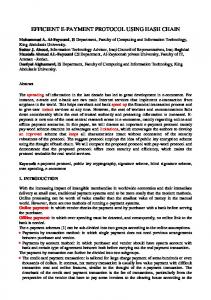
Design and Implementation of A Java Based Simulation Package for Spectrum Analysis, Digital Filtration and Modulation as A Teaching Aid for Data Communication Oluwole Oyetoke1, 2Dr. O.E Agboje 1, 2

Covenant University, Ota, Nigeria

Abstract: In the higher institutions of many third world countries, voids exist in the practical implementation of the engineering curriculum. Procuring the standard equipment for laboratory practical and student practice can at times be a financial burden to these institutions. This publication explains a fill to this void; by contributing a Java based Data Communication Simulation Package with which Communication Engineering students can conduct experiments over a Wi-Fi enabled network. These experiments are majorly in the areas of digital filtration, modulation and spectrum analysis. Keywords: Simulation, Modulation, Spectrum-Analyzer, Filtration.

I. INTRODUCTION In the manufacturing of modern day equipment, rigorous testing and analysis are done on the computer using simulation packages. These packages offer a wide range of application which saves manufactures the uphill task of having to assemble a complete hardware before experimenting or testing. The innovative idea of using simulators has established its root in the academics today. Widely adopted in universities today are computer laboratories where students can have virtual encounters with real life engineering devices and machines.

II. RELEVANCE AND APPLICATION OF THE PROJECT The theoretical section of coding schemes being taught in the classroom can be quite difficult to grasp hence the need for a simulation package to enhance comprehension of these concepts. A vital relevance of this project is its accessibility over a Wi-Fi network. Students outside the campus can be connected to the Virtual Laboratory via the extranet and by so doing, possess the capability of performing experiments at convenient times. The various applications of this project include distant learning purposes, teaching aid and communication engineering practical in open universities

III. METHODOLOGY A. PROGRAMMING STANDARD: The programming part of the project is done with respect to the X3J3 programming standard which stipulates 

Program Portability



Compatibility with existing standards and practice



Addition of desirable new features



Consistency and simplicity to the end user

Page | 30 Research Publish Journals

International Journal of Electrical and Electronics Research ISSN 2348-6988 (online) Vol. 3, Issue 1, pp: (30-41), Month: January - March 2015, Available at: www.researchpublish.com 

Compatibility for efficient implementation



Allowance for future growth



Acceptability for users

B. PROGRAM DESIGN PROCESS” This involves: 1.

Specifying the problem

2.

Analysing the problem

3.

Designing an algorithm

4.

Coding the algorithm into a suitable programming language

5.

Test the program

C. DESIGN APPROACH” The top down design approach was used. This involves considering the whole problem at the top level, split it into logical parts (modules). If possible, further split these modules into smaller units, until it can be easily passed through the program design process stated above. (Suggested by Yourdon, 1975). The master simulator as show in the block diagram below serves a guide for the methodology used in the implementation process.

Fig. 1. Block Diagram Of The Master Simulator

D. MEODULATION AND DEMODULATION MECHANISM: 1) MODULATION: Modulation is mapping information on a carrier. It is the process of facilitating the transfer of information over a medium [1]. There are various modulation techniques available, and these are: 

Amplitude Shift Keying (ASK) – The amplitude of the signal is changed in response to the information and every other thing is kept constant. On- off keying varies the amplitude between 0 and 1.



Frequency Shift Keying (FSK) – Frequency is varied



Phase Shift Keying (PSK) – Phase is varied

The term „shift keying‟ implies that they represent digital modulation. Binary phase shift keying (BPSK), Quadrature phase shift keying (QPSK), Quadrature amplitude modulation (16-QAM), Binary frequency shift keying (BFSK) are major modulation schemes.


International Journal of Electrical and Electronics Research ISSN 2348-6988 (online) Vol. 3, Issue 1, pp: (30-41), Month: January - March 2015, Available at: www.researchpublish.com a)

BPSK Modulation:

To modulate our 8 bit Baseband: 10101010, the converter converts all value „0‟ to „-1‟, meaning at every bit transition, the signal does a 180 degrees phase shift. The baseband input at this stage is 8 bits as a result of the hamming encoding and parity bit in the previous stage then we get 8 symbols which would be; s1, s2, s1, s2, s1, s2, s1, s2. A carrier with a free running frequency is then created. This serves as the packet of signal which we would use to multiply the baseband signal in order to get the modulated signal. (1) The carrier signal is an analogue signal of frequency fc. The modulation is then carried out by a vector multiplication of the two signals as shown below (2)

Fig. 2. Flowchart Illustrating The BPSK None Return to Zero (NRZ) Converter

b)

QPSK Modulation:

Unlike BPSK, QPSK uses two basic functions as the carrier. A sine and a cosine carrier. The dimensionality of modulation is dependent on the number of functions used [1]. By varying the phase of each of the carrier, two bits per symbol can be sent. Each symbol‟s phase is compared relative to the previous symbol; so, if there is no phase shift (0 degrees), the bits “00” are represented. If there is a phase shift of 180 degrees, the bits “11” are represented. In QPSK, there are four possible symbol positions where 2-bits each can be assigned to per time. To compute the QPSK modulation of our 8 bit baseband sequence: [1 0 1 0 1 0 1 0] Step1: Convert the bit sequence to a polar signal (i.e convert „0s‟ to „-1s‟) New sequence = [1 -1 1 -1 1 -1 1 -1] Step 2: Send alternating bits to In-phase and Quadrature phase channels. I = [1 1 1 1] Q = [-1 -1 -1 -1] Set the amplitudes of the I and Q based on the symbol mapping table above. Step 3: Multiply the I channel with a cosine function of frequency fc and the Q channel with a sine function. (a cosine function shifted by a 90 degrees would also do the job) Step 4: add the I and Q channels together and we get the modulated signal



Fig 3. Block Diagram of A QPSK Modulator

Fig 4. Flow Chart Showing QPSK Modulation

c)

16-QAM:

This is a type of ASK scheme, but has a PSK feature. The combined features are means to exploit both phase and amplitude shift keying. They have become more useful, in the advent of modern day transmission media such as fibre optics [2]. One signal is called the „I‟ signal, and the other is called the „Q‟ signal. Mathematically, one of the signals can be represented by a sine wave, and the other by a cosine wave. The two modulated carriers are combined at the source for transmission.



Fig: 5. Diagram of a 16-QAM Modulator [3]

The steps involved in the 16-QAM modulation technique are explained below Step1: Pass each chunk of 4 bits through a bit splitter (as in the diagram above) Step 2: Pass the Q, Q‟ and I, I‟ through the 2-to-4 Level Converter. The desired amplitude levels would be as specified in the table above Step 3: Modulate the output using the 2 carrier functions as in QPSK (SINE and COSINE) Step 4: Sum the output of the I and Q channel to produce the output The advantage of using QAM is that it is a higher order form of modulation and as a result it is able to carry more bits of information per symbol. With 16 QAM, you can carry as much as 4 bit per symbol. Since the 16- QAM takes 4 bits at a time, it gives us a possibility of using 16 different types of waves to represent the symbols. The table below show the various possible phase shifts, corresponding to various bit patterns. Shift the carrier relative to the previous wave, with respect to the taken in bit pattern. d)

BFSK Modulation:

Here, two discrete numbers of carriers are used to represent a binary input. The frequency of the carrier is alternated with respect to the value of the bit being transmitted {

( (

) )

}

(3)

Binary FSK is usually referred to simply as FSK. The data are transmitted by shifting the frequency of a continuous carrier in a binary manner to one or the other of two discrete frequencies. One frequency is designated as the “mark” frequency and the other as the “space” frequency. The mark and space correspond to binary one and zero, respectively. Some FSK terms are discoursed below. Element length: The minimum duration of a mark or space condition. An alternate way of specifying element length is in terms of the keying speed. The shift: The frequency difference between the mark and space frequencies. The nominal centre frequency: is halfway between the mark and space frequencies. Deviation: The deviation is equal to the absolute value of the difference between the centre frequency and the mark or space frequencies [4].


International Journal of Electrical and Electronics Research ISSN 2348-6988 (online) Vol. 3, Issue 1, pp: (30-41), Month: January - March 2015, Available at: www.researchpublish.com |

|

(4) (5) (6)

Step 1: Store baseband sample in an array Step 2: Generate 2 carriers each having distinct frequencies. Store carriers in two separate array. Step 3: Iterate through the baseband array, checking for binary 1s, replace those ones with the corresponding carrier value at that same spot Step 4: Iterate through the baseband array, checking for binary 0s, replace those ones with the corresponding carrier value at that same spot. Note: For this project, a higher frequency represents a 1 and a lower frequency represents a -1

Fig 6. Diagram of an FSK Modulator [5]

2) DEMODULATION: a)

BPSK Demodulation:

To demodulate BPSK, we multiply the incoming modulated signal with a carrier of the same frequency. The get this frequency, a PLL needs to be designed which would lock into the incoming signal, so as to determine the frequency. Designing the PLL is beyond the scope of this project. Therefore the already known frequency is used. The signal multiplied by the recovery carrier is integrated over a single bit period and then passed through a threshold detector for final analysis. The steps taken to program this are stated below (using 2048 samples of an 8hz modulated signal as case studies): Step 1; The entire incoming modulated signal is multiplied by a positive (+) and negative (-) carrier sample and stored in two separate arrays. Step 2: Samples per bit of the two categories of signals above are stored in various other arrays. Note: an 8bit/sec signal with 2048 samples would have 256 samples/bit, all stored in 8 different arrays Step 3: The first set 256 samples in category A are summed up and the first set of 256 samples in category B are also summed up. Step 4; the summation of category B is subtracted from the Summation of category A Step 5; if the subtraction is greater than zero, then bit „1‟ is detected. Otherwise, if the subtraction is less than zero, then bit „0‟ is detected as the output of the modulator.


International Journal of Electrical and Electronics Research ISSN 2348-6988 (online) Vol. 3, Issue 1, pp: (30-41), Month: January - March 2015, Available at: www.researchpublish.com Step 6; Return back to step 3 now using the next set of 256 bits. This iteration continues, until the entire 2048 samples are fully treated [6]

Fig: 7. Principal Of BPSK Demodulation [7]

b)

QPSK Demodulation:

The QPSK demodulation process is similar to that of the BPSK. The signal multiplied by the recovery carrier is integrated over a single bit period and then passed through a threshold detector for final analysis. The steps taken to program this are stated below (using 2048 samples of an 8hz modulated signal as case studies): Step 1; The entire incoming modulated signal is multiplied by a positive (+) and negative (-) carrier sample and stored in two separate arrays. Step 2: Samples per bit of the two categories of signals above are stored in various other arrays. Note; Since QPSK takes 2 bit at a time, the 8 bit modulated signal would consist of 4 bits. This four bits would translate to 1024 samples with 128 samples/ bit, and 256 samples representing 2 bits. Step 3: The first set 256 samples in category A are summed up (tagged set A) and the first set of 256 samples in category B are also summed up (tagged set B). Step 4; The groups of summed up bits are passed through a decision maker. In the decision maker, decisions are made as follows. TABLE: 1. QPSK Decision Table

Situation If (Set A0)

Decisions 00 01 10 11

Step 5; Return back to step 3 now using the next set of 256 bits. This iteration continues, until the entire1024 samples are fully treated.

Fig: 8. Block Diagram of A QPSK Demodulator [8]


International Journal of Electrical and Electronics Research ISSN 2348-6988 (online) Vol. 3, Issue 1, pp: (30-41), Month: January - March 2015, Available at: www.researchpublish.com c)

FSK Demodulation:

The demodulation methods for FSK can be divided into two major categories: FM detector demodulators and filter-type demodulators.

Fig. 8: FSK Non Coherent Receiver [8]

The Sampling and Judge Process involves the following step (using 2048 samples of an 8 Hz modulated signal as case studies). Step 1: Empty the array of the FSK modulated signal into 8 other arrays, each representing a sampled bit. Step 2: Compute the FFT of the 8 arrays individually. The FFT of these arrays would give spikes at frequencies corresponding to the frequency of the carrier wave. Recall that the FSK uses deviation in frequency to represent a baseband signal. By the reason of this, you should detect two distinct frequency components from the FFT analysis. Step 3: The larger frequency component represents a 1 (mark) and the lower on represents a -1 (space). d)

16-QAM DEMODULATION:

QAM is demodulation is achieved by using the same process used in the modulator, but in reverse. This gives it the advantage of being able to use existing PSK modulator and demodulator circuits. The 16-QAM receiver is an exact inverse of the 16-QAM transmitter. E. FILTRATION MECHANISM: This simulator employs the FIR class of filters, under which various kinds of filters would be used. These filter kinds include: 

Low - Pass



Band - Pass



High - Pass and



Band – Stop Filters

1) Finite Impulse Response Filter (FIR): A finite impulse response filter is one whose impulse response is finite i.e its response settle back to zero in a finite time frame. The impulse response of an Nth-order discrete-time FIR filter lasts for N + 1 samples, and then settles to zero. 2) Filter Design Stages: 1.

Filter Specification

2.

Co-efficient Calculation

3.

Structure selection


International Journal of Electrical and Electronics Research ISSN 2348-6988 (online) Vol. 3, Issue 1, pp: (30-41), Month: January - March 2015, Available at: www.researchpublish.com a)

Filter Specification:

(1)

Low Pass Filter

These filters basically allow low frequency signals to pass through and on the other hand stop high frequency signals. The impulse response of an ideal low-pass filter is a SINC function. Unfortunately, given a non recursive filter structure, the SINC function is infinite in the x-direction; however, the FIR filter only allows us to have a finite impulse response. This is why we need to apply the window function. Therefore only a portion of the impulse is actually used and secondly the impulse response is shifted so the filter only operates on available samples [9]. The co-efficients of a low-pass filter is given to be: ( (

(2)

)

(7)

( ))

High Pass Filter: –

(8)

These filters basically are filters that pass frequencies above a certain value and attenuate frequencies below that value. The order of the filter must be even [10]. The co-efficients is given by the expression: ( (

(3)

( ))

{

)

(

}

)

(9)

Band Pass Filter:

A band-pass filter is a device that passes frequencies within a certain range and rejects frequencies outside that range. Optical band-pass filters are of common usage. An example of an analogue electronic band-pass filter is an RLC circuit [11]. These filters can also be created by combining a low pass filter and a high pass filter. The co-efficients of the filter is given by the expression: ( (

( ))

{

(

( (4)

)

(

)

(

)

} (10)

)

)

Band Stop Filter:

In signal processing, a band-stop filter or band-rejection filter is a filter that passes most frequencies unaltered, but attenuates those in a specific range to very low levels. It is the opposite of a band-pass filter. A notch filter is a band-stop filter with a narrow stop band. The filter order must be even [12]. The co-efficient of the filter is given by the expression:

( (

( ))

{

(

(

) )

( (

) )

} (11)

)

NOTE: The co-efficient of a filter are the same as the impulse response samples of a filter (5)

Kaiser Window:

Here the amount of ripple and transition bandwidth need to be specified. This method is not considered in this project. b)

Co-efficient Calculation:

Various methods can be used with include 

Windowing Method



Frequency sampling



Parks-Mc Cllelan method


International Journal of Electrical and Electronics Research ISSN 2348-6988 (online) Vol. 3, Issue 1, pp: (30-41), Month: January - March 2015, Available at: www.researchpublish.com The scope of this project is using the windowing method which is explained below. First calculate the co-efficients of the Filter using the equation in method 1 above. Second stage of this method is to select a window function. Various Windows include (1)

Rectangular Window:

The rectangular window has excellent resolution characteristics for signals of comparable strength. The rectangular window is defined as ( ) (2)

{

}

(12)

Hamming Window:

The Hamming window is, like the Hanning window, also a raised cosine window. The Hamming window exhibits similar characteristics to the Hanning window but further suppress the first side lobe. ( ) (3)

–

(13)

Hanning Window:

The Hanning window is a raised cosine window and can be used to reduce the side lobes while preserving a good frequency resolution compared to the rectangular window. It is commonly used as general purpose window for the analysis of continuous signals. ( ) (4)

(

)

(14)

Barlet Window:

A Bartlett window is a triangular shaped window function. The Bartlett window has higher side lobe attenuation than the rectangular window. ( ) (5)

–

|

|

(15)

Blackman Window:

The Blackman window is similar to the Hanning and the Hamming windows. An advantage with the Blackman window over other windows is that it has better stop band attenuation and with less pass band ripple. The Blackman window is defined as: ( )

(16)

The third stage is to calculate the set of truncated or windowed impulse response coefficients ( ) As was mentioned earlier, because ( ) is of infinite duration (infinite along the x-axis), the samples must be truncated. Truncation is performed by multiplying desired sample response with a window function in time domain which gives sample response of filter represented as ( ) Where

( )

( )

(17)

( ) is the corresponding impulse response (filter co-efficient) and

( )is a window function.

c) Structure Specification: This would be needed in the event of designing a hardware filter. 3) Definition of Filter Variables: M = Filter length i.e order of filter. One is subtracted from this value if the number of samples is odd. This is done to make the M value = an even number (18) n = weight, it ranges from 0 to M


International Journal of Electrical and Electronics Research ISSN 2348-6988 (online) Vol. 3, Issue 1, pp: (30-41), Month: January - March 2015, Available at: www.researchpublish.com 4) Filtration Proper: Filtration is attained by simple convolution in time domain of the filter coefficients and the input sequence. This is otherwise known as linear convolution. On the other hand, filtration can also be attained by the circular convolution. The steps for the circular convolution method are as follows: Step 1: Get the impulse response of the filter (h) in use and the sample signal in use (x) Step 2: Compute the FFT of the two signals Step 3: Compute the complex multiplication of the two FFT sequence Step 4: Compute the complex Inverse FFT of the sequence gotten from step 3 above The real part of your output in step 4 above is your filtered signal ( a)

((

( )

( )))) (19)

Using linear Convolution:

The response of an LTI discrete time system to an arbitrary input sequence is given by the convolution summation of the input sequence and the impulse response sequence of the filter. The fast Fourier transform of the convolution of two time sequence is equal to the product of the fast Fourier transform sequence. To find the time response of the system, compute the inverse fast Fourier transform. In the equation below, N represents the order of filter. ∑

(20) ,

F. FREQUENCY RESPONSE ANALYSIS: The time response of a system is not sufficient enough to characterize the performance of the system. This is because the frequency is not considered. However, in frequency response analysis, the frequency is considered. To do this, this project employs the „divide and conquer algorithm‟ of the Fast Fourier Transform. By computing the fast Fourier transform of a sequence of numbers in the time domain, the realization of its spectrum in the frequency domain can be obtained. An already written Java class for Fast Fourier analysis by the University of Columbia. G. WEB BROWSER SYNCHRONIZATION: Making the simulation package accessible over a web browser was achieved via the Java web start.

IV. IMPLEMENTATION

Fig: 9. Snapshot of the master simulator’s GUI


International Journal of Electrical and Electronics Research ISSN 2348-6988 (online) Vol. 3, Issue 1, pp: (30-41), Month: January - March 2015, Available at: www.researchpublish.com V.

CONCLUSION

Simulation based learning has proven to be a methodology implementable in virtually any field of study. The fact that simulators are currently available which can perform complex modulation, filtration and spectrum analysis validates the fact that virtual experimentation is highly feasible in the field of engineering. This simulation package can now be implemented in laboratories which have challenges in procuring the needed hardware/equipment. ACKNOWLEDGEMENT I would like to acknowledge my project supervisor, Dr. O. E Agboje whose strong project management and co-ordination skills helped me see this project through. He instilled in me the spirit of resilience. REFERENCES [1]

All about modulation part 1, www.complextoreal.com, retrieved 20th January, 2014.

[2]

Dr. O.E Agboje, Digital Modulation Schemes, Lecture Note 5, 2011.

[3]

Mehran University of Engineering and Technology, Examination 2009 Batch 7.

[4]

FSK Demodulation, WJ Tech Notes 1980Tech-notes, Vol. 7 No. 5 September/October 198 Watkins-Johnson Company, Copyright © 1980 Watkins-Johnson Company.

[5]

A Software Defined Radio Implementation Using MATLAB, by Ziyi Feng, Master‟s Thesis, 2013.

[6]

Nehal. A. Ranabhatt, Sudhir Agarwal, Priyes H. P. Gandhi, “RTL Design and implementation of BPSK Modulation at Low Bit Rate”, International Journal of Engineering Research and Technology, ISSN:2278-0181, Vol.2, Issue 23, Feb 2012.

[7]

A. Spanias, V. Atti, “Interactive online undergraduate laboratories using “J-DSP,” IEEE Transactions on Education, vol. 48, no. 4, pp. 735- 749, Nov. 2005.

[8]

Agboje, O.E., a PhD Thesis on “Computer Simulation of Digital Modems for Satellite Mobile Communications”, Page 10, University of Bradford, Bradford, UK, 1991.

[9]

Low Pass Filter, www.labbookpages.co.uk/audio/firWindowing.html, retrieved 17th January, 2014.

[10]

High Pass Filters, http://wordnetweb.princeton.edu/perl/webwn?s=high-pass filter, retrieved; 17th January, 2014.

[11]

Band Pass Filter, http://en.wikipedia.org/wiki/Band_pass_filter, retrieved; 17th January, 2014.

[12]

Band Stop Filter, http://en.wikipedia.org/wiki/Band-stop_filter, retrieved; 17th January, 2014.


Design and Implementation of A Java Based Simulation Package for ...

Design and Implementation of A Java Based Simulation Package for ...

Suggest Documents