School of Electrical, Electronic & Computer Engineering
Design and Measurement of Synchronizers by
Jun Zhou
Technical Report Series NCL-EECE-MSD-TR-2008-138
November 2008
Contact:
[email protected] EPSRC supports this work via EP/C007298/1 (SYRINGE)
NCL-EECE-MSD-TR-2008-138 Copyright © 2008 Newcastle University
School of Electrical, Electronic & Computer Engineering, Merz Court, Newcastle University, Newcastle upon Tyne, NE1 7RU, UK
http://async.org.uk/
University of Newcastle upon Tyne School of Electrical, Electronic and Computer Engineering
Design and Measurement of Synchronizers
by
Jun Zhou
A thesis submitted for the degree of Doctor of Philosophy (Ph.D) at Newcastle University
November 2008
Content List of Publications
ix
List of Figures
x
List of Tables
xiii
Acknowledgements
xiv
Glossary of Abbreviations
xv
Abstract
xvi
1. Introduction
1
1.1 Background ....................................................................................................... 1 1.2 Synchronizer Issues........................................................................................... 4 1.3 Contributions..................................................................................................... 7 1.4 Thesis Structure................................................................................................. 9
2. Literature Review
11
2.1 Synchronizer ................................................................................................... 11 2.1.1 Why are synchronizers needed................................................................. 11 2.1.2 How are synchronizers used?................................................................... 14 2.2 Synchronizer modelling .................................................................................. 16 2.2.1 Metastability............................................................................................. 16
iv
2.2.2 Resolution of Metastability in Synchronizers .......................................... 21 2.2.3 Synchronizer Failure Rates ...................................................................... 24 2.3 Synchronizer Circuits...................................................................................... 29 2.3.1 Latches ..................................................................................................... 29 2.3.2 Jamb Latch ............................................................................................... 30 2.3.3 Other proposed synchronizers.................................................................. 32 2.4 Synchronizer Simulation and Measurement ................................................... 37 2.4.1 Synchronizer Simulation.......................................................................... 37 2.4.2 Synchronizer Measurement...................................................................... 39 2.5 Effects of On-chip Variability on Synchronizers............................................ 46
3. Robust Synchronizer
48
3.1 Jamb Latch ...................................................................................................... 49 3.2 Modified Jamb Latch ...................................................................................... 55 3.3 Improved Synchronizer (Robust Synchronizer).............................................. 58 3.4 Summary ......................................................................................................... 62
4. On-chip Measurement of Deep Metastability in Synchronizers
64
4.1 Measurement of Metastability in Synchronizers............................................. 65 4.1.1 Traditional Measurement Methods .......................................................... 66
v
4.1.2 On-chip Deep Metastability Measurement .............................................. 68 4.2 Implementation of On-chip Deep Metastability Measurement....................... 69 4.2.1 Variable Delay Lines................................................................................ 70 4.2.2 Devices Under Test (synchronizers) ........................................................ 73 4.2.3 Control Logic ........................................................................................... 74 4.2.4 Layout of On-chip Measurement Circuit ................................................. 78 4.3 Measurement Results ...................................................................................... 79 4.3.1 Input Histogram ....................................................................................... 79 4.3.2 Output Histogram..................................................................................... 79 4.3.3 Corrected Input Histogram....................................................................... 81 4.3.4 Input Time vs Output Time...................................................................... 84 4.3.5 Tau vs Vdd ............................................................................................... 87 4.4 Summary ......................................................................................................... 88
5. Adapting Synchronizers to the Effects of On-chip Variability
90
5.1 On-chip Measurement of Failure Rates .......................................................... 93 5.2 Calculation of and MTBF............................................................................. 94 5.2.1 Calculate from Measured Failure Rates ................................................ 94 5.2.2 Calculate MTBF from Measured Failure Rates ....................................... 95 5.3. Two Proposed Adaptation Schemes............................................................... 96
vi
5.3.1 Synchronizer Selection Scheme............................................................... 96 5.3.2 Synchronization Time Adjustment Scheme............................................. 98 5.4 Implementation ............................................................................................. 100 5.4.1 Architecture of Synchronizer Selection Scheme.................................... 100 5.4.2 Architecture of Synchronization Time Adjustment Scheme ................. 102 5.4.3 Failure Detector...................................................................................... 104 5.4.4. Failure Counters .................................................................................... 104 5.4.5 Synchronizer Selection Circuit .............................................................. 105 5.4.6 Variable Delay Line ............................................................................... 106 5.4.7 Implementation of and MTBF Calculation ........................................ 107 5.4.8 Hardware Saving.................................................................................... 110 5.5 Applications of Two Schemes ...................................................................... 111 5.6 Test Results ................................................................................................... 112 5.7 Summary ....................................................................................................... 114
6. Conclusions and Future Work
116
6.1 Conclusions ................................................................................................... 116 6.2 Future Work .................................................................................................. 123
vii
Appendix A. TSMC 0.18μm SPICE Parameters from MOSIS
125
Appendix B. UMC 0.18μm/90nm SPICE Parameters from Europractice
127
Bibliography
129
viii
List of Publications 1. J. Zhou, D. J. Kinniment, G. Russell, and A. Yakovlev, “Adapting Synchronizers to the Effects of On Chip Variability”, 14th IEEE International Symposium on Asynchronous Circuits and Systems, pp. 39-47, 2008. 2. J. Zhou, D. J. Kinniment, G. Russell, and A. Yakovlev, “On-Chip Measurement of Deep Metastability in Synchronizers”, IEEE Journal of Solid-State Circuits, Vol. 43, No. 2, pp. 550-557, 2008. 3. J. Zhou, D. J. Kinniment, G. Russell, and A. Yakovlev, “A Robust Synchronizer Circuit”, IEEE Computer Society Annual Symposium on VLSI, pp. 442-443, 2006. 4. J. Zhou, D. J. Kinniment, G. Russell, and A. Yakovlev, “On-chip Measurement of MTBF for A Robust Synchronizer”, 19th UK Asynchronous Forum, 2007. 5. H. Ramakrishnan, S. Shedabale, J. Zhou, G. Russell, and A. Yakovlev, “Variability analysis of a high performance strained silicon Jamb latch synchronizer”, 19th UK Asynchronous Forum, 2007.
ix
List of Figures Figure 2.1 Metastability in flip-flop.......................................................................... 12 Figure 2.2 Two flip-flops synchronizer .................................................................... 13 Figure 2.3 GALS system........................................................................................... 15 Figure 2.4 Synchronizers in system .......................................................................... 16 Figure 2.5 D Latch .................................................................................................... 17 Figure 2.6 Metastable state ....................................................................................... 18 Figure 2.7 Metastable equilibrium ............................................................................ 19 Figure 2.8 Metastable outputs [20] ........................................................................... 20 Figure 2.9 Metastable events and output histogram.................................................. 20 Figure 2.10 Small signal models of gate and flip-flop.............................................. 22 Figure 2.11 Occurrence and resolution of metastability ........................................... 25 Figure 2.12 Input time and output time relationship................................................. 27 Figure 2.13 Latches based synchronizer ................................................................... 29 Figure 2.14 Latch with filter ..................................................................................... 30 Figure 2.15 Structure of Jamb latch .......................................................................... 31 Figure 2.16 Metastability blocker [31]...................................................................... 34 Figure 2.17 Metastability shaker............................................................................... 35 Figure 2.18 Low input coupling latch [27] ............................................................... 36 Figure 2.19 Switch method ....................................................................................... 38 Figure 2.20 Two-oscillator measurement method .................................................... 40 Figure 2.21 Deep metastability measurement........................................................... 41 Figure 2.22 Input and output histograms .................................................................. 42 Figure 2.23 Input time to output time ....................................................................... 43
x
Figure 2.24 Analog implementation of deep metastability measurement [38]......... 45 Figure 3.1 Jamb latch ................................................................................................ 49 Figure 3.2 Simulating Jamb latch.............................................................................. 51 Figure 3.3 Diverging nodes....................................................................................... 52 Figure 3.4 Semilog plot of the voltage difference of the two nodes ......................... 52 Figure 3.5 Plot of vs Vdd for Jamb latch ................................................................. 53 Figure 3.6 Energy consumption ................................................................................ 54 Figure 3.7 Synchronization time constant .............................................................. 55 Figure 3.8 Modified Jamb latch ................................................................................ 56 Figure 3.9 Plot of vs Vdd for modified Jamb latch.................................................. 57 Figure 3.10 Improved synchronizer (robust synchornizer)....................................... 58 Figure 3.11 Plot of vs Vdd for improved synchronizer ........................................... 60 Figure 3.12 Improved synchronizer, input vs output time at 1.8v ............................ 61 Figure 3.13 Improved synchronizer, input time vs output time at 0.9V ................... 62 Figure 4.1 Traditional measurement method using two oscillators .......................... 66 Figure 4.2 Typical event histogram [38]................................................................... 67 Figure 4.3 Deep metastability measurement............................................................. 68 Figure 4.4 Traditional VDL ...................................................................................... 70 Figure 4.5 Improved VDL......................................................................................... 72 Figure 4.6 Multiplexer circuit for DUTs................................................................... 74 Figure 4.7 Controlling counters ................................................................................ 75 Figure 4.8 Loading circuit for controlling counters .................................................. 76 Figure 4.9 Generation of RESET signal ................................................................... 77 Figure 4.10 Layout of on-chip measurement circuit................................................. 78 Figure 4.11 Input histogram...................................................................................... 79
xi
Figure 4.12 Output histogram ................................................................................... 80 Figure 4.13 High output events vs low output events............................................... 81 Figure 4.14 Measurement of actual input time distribution...................................... 82 Figure 4.15 Corrected input histogram ..................................................................... 83 Figure 4.16 Measured Input time (s) vs output time (ns).......................................... 85 Figure 4.17 Simulated input time (s) vs output time (ns) ........................................ 86 Figure 5.1 On-chip measurement of failure rates...................................................... 94 Figure 5.2 Architecture of Synchronizer Selection Scheme ................................... 101 Figure 5.3 Architecture of Synchronization Time Adjustment Scheme ................. 102 Figure 5.4 Failure counters ..................................................................................... 105 Figure 5.5 Synchronizer Selection Circuit .............................................................. 106 Figure 5.6 Variable delay line................................................................................. 107 Figure 5.7 Calculation flow..................................................................................... 108 Figure 5.8 Divider ................................................................................................... 109 Figure 5.9 Log calculation circuit ........................................................................... 110 Figure 5.10 Calculated MTBF vs Data Rate (Synchronization Time=3.5ns, Clock Frequency=10MHz) ................................................................................................ 112 Figure 5.11 Calculated MTBF vs Synchronization Time (Data Rate=5MHz, Clock Frequency=10MHz) ................................................................................................ 113 Figure 5.12 Tau vs Vdd........................................................................................... 113
xii
List of Tables Table 4.1 Tau vs Vdd for Jamb B and Robust Synchronizer………….…………...87 Table 5.1 Jamb latch vs Vdd at 90nm…………………………………………….98
xiii
Acknowledgements I would like to express my gratitude to my supervisors, Dr Gordon Russell and Professor Alex Yakovlev for their patient guidance, kind encouragement and constant support in all the time of my PhD research and writing of this thesis. I am deeply indebted to Professor David Kinniment for his tremendous help and valuable suggestions during my research. His deep knowledge of synchronizer and logical way of thinking have been of great value to me. Without his help this work could not have been done. I would like to acknowledge the support from EPSRC grant EP/C007298/1 and Intel Corporation. Special thanks to Charles Dike from Intel for his valuable suggestions in my research work. I am grateful to my colleagues who have helped me in last three years. I want to thank Julian Murphy for his introduction of the usage of EDA tools. I have furthermore to thank Nikolaos Minas and Hiran K Ramakrishnan with whom I had a many valuable discussions on my research work and writing of thesis. My special thanks go to Yuan Chen, Yu Zhou, Ping Wang and Jincheng Zhu who have offered me a lot of help and made my life in UK interesting. Especially, I would like to give my special thanks to my parents whose constant love and support enabled me to complete this work.
xiv
Glossary of Abbreviations DLL
Delay Locked Loop
DPE
Data Processing Engine
DUT
Device Under Test
DVFS
Dynamic Voltage & Frequency Scaling
GALS Global Asynchronous and Local Synchronous MTBF
Mean Time Between Failure
SoC
System on Chip
VDL
Variable Delay Line
xv
Abstract Future Systems on Chip (SoCs) are likely to consist of many independent or semi-independent clock regions with the need to synchronize the data passing between them. Consequently, there will be many synchronizers together with interconnecting and routing elements forming an on-chip communication network. Due to the rapidly increasing size of SoCs in terms of the number of IP cores on a single chip, the on-chip communication is likely to impact on the system performance more than processing. As an important part of on-chip communication network, the performance of synchronizers on chip is critical to the performance of the entire system. To address the issues of the effects on performance resulting from the inclusion of synchronizers in SoCs, several aspects related to synchronizer design and measurement need to be investigated; to date these aspects have either not been considered or inadequately addressed. A common problem with synchronizers is that their performance degrades rapidly with decreasing Vdd and is sensitive to Vdd, Vth and temperature variations. Another problem is that the existing synchronizer simulation and measurement techniques are not sufficiently accurate for estimating synchronizer performance to predict long term mean time between failures (MTBF). In addition, synchronizer performance is heavily affected by the on-chip variability, which needs to be addressed as the on-chip variability issue becomes more and more significant in deep submicron process technologies.
xvi
This thesis investigates the above issues and proposes solutions to each of them. Based on the commonly used Jamb latch synchronizer, a novel synchronizer circuit, which is able to work at low Vdd and is robust to Vdd, Vth and temperature variations, has been proposed. The simulation and measurement results show that the robust synchronizer only consumes slightly higher power than the Jamb latch, but it is much faster when working at low Vdd and much less sensitive than the Jamb latch to Vdd, Vth and temperature variations. An on-chip measurement circuit, which can measure deep metastability in synchronizers, has been designed and fabricated with a 0.18μm process. The measurement results show that the measurement method works stably and provides reliable results into the deep metastability region for predicting long term MTBF. Two adaption schemes have also been proposed to greatly mitigate the effects of on-chip variability on synchronizer performance. Their feasibility has been demonstrated using FPGA, showing that they work as expected.
xvii
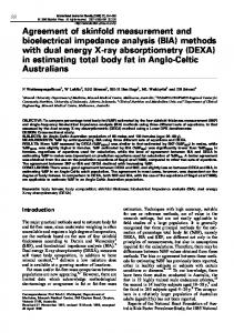
Chapter 1 Introduction 1.1 Background The System on Chip (SoC) emerged as a design concept as early as 2002 and was considered as the ideal replacement for multichip solutions. In general SoCs include multiple CPU cores, on-chip memory, and interconnections between them, along with built-in I/O interfaces as shown in Figure 1.1.
Figure 1.1 Achitecture of SoC [1]
1
Compared to multichip solutions, the SoC has the following advantages: 1. Better system performance 2. Lower power consumption 3. Greater functionality 4. Smaller system size 5. Lower part counts Using SoCs can shorten development cycle while increasing product functionality, performance and quality. Due to the above advantages, SoCs have been applied in many areas such as consumer electronics, medical electronics, networking and communication, automotive and defence. The goal of SoC design is to maximize reuse of existing functional blocks or IP cores by increasing levels of the integration. Figure 1.2 shows the trend of SoC design complexity predicted in ITRS 2007 [1]. Here, a Data Processing Engine (DPE) is a processor dedicated to data processing which achieves high throughput by eliminating general purpose features. A main processor is a general purpose processor which allocates the schedules jobs to DPEs.
2
Figure 1.2 Trend of SoC design complexity [1] Due to the ever growing size of SoCs, plus increasing clock frequency and shrinking device dimensions, it has become difficult or impossible to accurately distribute a single global clock across the entire chip [2][3][16]. In addition, as power saving techniques such as dynamic voltage and frequency scaling (DVFS) are widely used, different parts of the SoC are required to run at different frequencies to reduce the power consumption [4]. Future SoCs are likely to consist of many independently or semi-independently clocked regions, which are known as global asynchronous
and
local
synchronous
(GALS)
systems
[5][6][7][8][9].
Synchronization is needed for data passing between different clock regions in GALS systems, otherwise metastability will occur which may lead to severe system failures. Using synchronizers in interfacing different clock regions is a simple and economical solution to the synchronization issue in GALS systems. Instead of avoiding metastability, this solution is to leave some time for metastability to resolve itself in the synchronizer before it is sampled by subsequent circuits, so as to
3
reduce the probability of metastability being transferred to the next circuit. Consequently the mean time between failures (MTBF) is increased [27].
1.2 Synchronizer Issues Future SoCs are likely to consist of many synchronizers on a single chip as the number of IP cores incorporated increases. For example, in a 64-core processor system, at least 128 synchronizers are needed by considering that one core needs at least two synchronizers for its input and output. In future SoCs, the on-chip communication including synchronization, routing and buffering is likely to affect the system performance more than processing [18]. As a critical part of on-chip communication network, the performance of the synchronizers on chip is crucial to the performance of the entire system. The simplest synchronizer comprises two flip-flops. Metastability may occur at the first flip-flop. Then a full clock cycle is used for the metastability to settle. MTBF can be increased by increasing the clock period which is the synchronization time. However, the resolution of metastability in a two flip-flop synchronizer is relatively slow, which makes it unsuitable for high speed applications where clock frequencies are high. In the past, many different synchronizers with improved performance have been proposed [24][27][28][31][32][33][34]. However, they have a common problem, that is the synchronizer performance degrades rapidly with Vdd decreasing or Vth increasing because the synchronization time constant, , which determines the synchronizer performance depends on the small signal behaviour of the bistable element in the synchronizers. This situation is aggravated by lowering the temperature which results in a higher threshold voltage. Consequently, the
4
synchronizer performance is sensitive to Vdd, Vth and temperature variations. With the wider use of power saving techniques such as DVFS and the advances in process technology, Vdd will become lower and lower where synchronizers may fail to work. In addition, increasing on-chip variability could significantly degrade the synchronizer performance. Therefore, it is necessary to design synchronizers which are able to work at low Vdd and are robust to the Vdd, Vth and temperature variations. The synchronizer performance can be estimated either by simulation or measurement. The simulation methods [24][37] are not sufficiently accurate for estimating synchronizer performance in the deep metastability region, which is the region for long metastability and is used to predict long term MTBF, because the resolution of simulators is limited and some devices exhibit variations in τ in the deep metastability region. Another disadvantage of the simulation methods is that noise may be important for the nondeterministic part of the synchronizer response, and so the result of a deterministic simulation may or may not be a true representation of the results in practice. The traditional measurement methods [24][28][29][30] using two oscillators are not accurate either for measuring synchronizer performance in the deep metastability region because different overlap times are generated at equal probabilities and thus deep metastability events that correspond to very short overlap times have a very small probability of occurrence. Even when they occur, it is not necessary that they can be recorded because the response speed of the oscilloscope used to record the metastability events is limited, which makes it more difficult to measure synchronizer performance in the deep metastability region. To cope with the above problems, a new measurement method has been proposed recently [36]. It greatly increases the probability of occurrence of deep metastability events by forcing the data to come close to the balance point by
5
using a delay locked loop (DLL). However, the method was implemented using offchip analogue circuits, which makes it difficult to control the operation of variable delay lines or to characterise the actual input time distribution due to the instability of the off-chip analog components. It is also difficult to achieve an incremental delay of pico-second levels with an off-chip analogue delay line. These problems can be overcome by implementing the deep metastability measurement method on chip using digital variable delay lines and digital counters. On-chip variability such as process, voltage and temperature variations is becoming an important issue on the performance of systems on silicon as the size of SoCs increases and the process technology advances [1]. Components such as logic circuits, memories on chip are all affected, but the performance of synchronizers which are used to synchronize data passing between different clock regions in future SoCs may affect the system performance to a greater extent than other components because the synchronizer performance depends on small signal rather than large signal behaviours and synchronization is a critical part of the on-chip communication which is likely to affect the system performance more than processing as the size of SoCs increases and the device dimensions shrink. Developing transistor level design techniques for more robust synchronizers [23] can be a way to improve the performance of the synchronizer as well as reducing its sensitivity to process, voltage and temperature variations, but all synchronizers exhibit variability. The synchronizer performance can be further enhanced using system level design techniques. Recently adaptation schemes have been used to mitigate the effect of process variation in microprocessor designs [43]. Similar ideas can be applied to synchronizer circuits to reduce the effects of on-chip variability on synchronizer performance.
6
1.3 Contributions To address the above issues, research has been conducted in synchronizer design, measurement and performance variability, and the following contributions have been made through the research. 1) Based on the commonly used Jamb latch synchronizer, modifications have been made and an improved synchronizer which is able to work at very low Vdd and is robust to the Vdd, Vth and temperature variations has been proposed. The Jamb latch was first modified to be much less sensitive to Vdd variations. However, this led to a significant increase in the power consumption. Thereafter in an improved synchronizer a technique was used to reduce the power consumption while maintaining its robustness. The simulation and measurement results show that, for the improved synchronizer, the switching energy required is only a little higher than the Jamb latch, but it is much faster when working at low Vdd and much more robust than the Jamb latch to the Vdd, Vth and temperature variations. This work has been published in the 2006 IEEE Computer Society Annual Symposium on VLSI [23] and is presented in Chapter 3. 2) An on-chip measurement circuit using deep metastability measurement method for measuring synchronizer performance has been designed and fabricated using UMC 0.18µm technology along with the devices under test (the Jamb latch synchronizer and the proposed robust synchronizer). A delay locked loop comprising digital variable delay lines and digital counters is used to force the data for the synchronizer to come close to the clock so as to increase the probability of occurrence of deep metastability events.
7
Compared with the previous off-chip implemention using analog circuits, the on-chip implementation using digital circuits allows integration of both the synchronizer circuits and the measurement method, and eliminates high speed off-chip paths which are a source of inaccuracy. It also makes control at the picosecond level easier because of the inherent stability of digital integrating counters and digital delay lines. The measurement results show that the on-chip deep metastability measurement method is stable and reliable, the data for the synchronizer is closely locked to the clock and can be measured in the deep metastability region. The measurement results also show that the tested devices are slower in the deep metastability region than they are in the deterministic region. For this reason the simulation which is only reliable for estimating the early part of synchronizer response cannot be relied upon to predict MTBF at realistic synchronization times, and it is necessary to check the value of in deep metastability with accurate measurement. In addition, a comparison was made between the Jamb latch and the robust synchronizer at different Vdd. The measurement results validated the previous simulation results, showing that the robust synchronizer circuit is much faster than the Jamb latch at low Vdd and is robust to Vdd variation. This work has been published in the IEEE Journal of Solid-State Circuits [39] and is presented in Chapter 4. 3) Two adaptation schemes used to mitigate the effects of on-chip variability on synchronizer performance have been proposed. Their feasibility has been demonstrated using an FPGA. The first scheme, namely Synchronizer Selection Scheme, is used to improve the synchronizer performance subject to process variation by selecting the best synchronizer to use out of a number
8
of synchronizers. Compared to simply increasing the transistor size in the synchronizer, this scheme can further reduce the effects of process variation and significantly reduce the power consumption. The second scheme, namely Synchronization Time Adjustment Scheme, is targeted at overdesigned synchronization times due to synchronizer performance variability caused by on-chip variability. It is used to improve the system performance by adjusting the synchronization time according to the actual process, voltage, temperature and data rate variations on the condition that the required MTBF is met. Assuming that the synchronization time constant τ which determines the resolution speed of metastability in synchronizers can increase by 25% due to process variation and a further 25% due to Vdd and temperature variations, this scheme can improve the performance of the system by 33%. This work has been published in the 14th IEEE International Symposium on Asynchronous Circuits and Systems [44] and presented in Chapter 5.
1.4 Thesis Structure Having discussed the motivations and contributions of the research the roadmap for the remainder of the thesis is outlined below. An overview of the main issues in current synchronizer research is outlined in Chapter 2. It first introduces why and how synchronizers are used. Then the theory of metastability and synchronization is reviewed. After that some of the existing synchronizer circuits are investigated and the common problems in synchronizer design are discussed. Next the existing simulation and measurement methods for
9
synchronizers are studied and their problems are discussed. Finally the effects of onchip variability on synchronizer performance are studied and its impact on system performance is analyzed. In Chapter 3 the commonly used Jamb latch synchronizer is investigated. A modified version of the Jamb latch is presented, which is much less sensitive to Vdd, Vth and temperature variations but consumes more power. Next a novel synchronizer circuit, which is both faster and much more robust than the Jamb latch while at the same time maintaining low power consumption, is presented. Finally the improvement resulting from the proposed synchronizer is summarized. The on-chip measurement of deep metastability in synchronizers is described in Chapter 4. Initially the traditional measurement methods are reviewed and the principle of on-chip deep metastability measurement is described together with the implementation of the on-chip measurement circuit. Next, the measurement results are shown and a comparison is made with the simulation results, demonstrating that the on-chip measurement method is stable and reliable. In Chapter 5 the two adaptation schemes proposed to reduce the effects of onchip variability on synchronizer performance are described. Initially the on-chip measurement of failure rates is discussed, followed with an explanation of how τ and MTBF are calculated from the failure rates. Subsequently the synchronizer selection scheme and synchronization time adjustment scheme are described, followed by the implementation details of the two adaptation schemes. Next the applications of the two adaptation schemes are discussed and the test results are presented.
10
The conclusions resulting from the work undertaken in the thesis together with future work are presented in Chapter 6.
Chapter 2 Literature Review 2.1 Synchronizer This section introduces why synchronizers are needed and how they are used.
2.1.1 Why are synchronizers needed As the size of SoCs in terms of the number of modules incorporated increases and the process technology shrinks, it has become more and more difficult to accurately distribute a single global clock across the entire systems. Skew and jitter in both the clock and the data mean that the system may have to be divided into many subsystems, which are either independently clocked or at least semiindependent. In addition, in a multiple IP cores SoC, different IP cores are required to run at different frequencies in order to achieve low power and maximum performance. As a response to these challenges, GALS architectures which allow the reuse of synchronous IP cores in an asynchronous environment have been proposed and investigated [5][6][7][8][9]. In a GALS system, different cores are optimised to operate at different frequencies to achieve low power and maximum performance, and therefore form many different clock regions. Synchronization is needed for data passing between 11
different clock regions [10]. To understand this, let us look at a flip-flop. As shown in Figure 2.1, data from a different clock region is seen as an asynchronous signal by the flip-flop. It can arrive any time. When it arrives very close to the rising edge of the local clock and violates the setup condition, metastability may occur at the output of the flip-flop (which is explained in detail in Section 2.2.1). Metastability is often seen as an indeterminate level between logic 0 and logic 1 which may cause failures in subsequent circuit blocks which are designed only for defined logic levels. When metastability occurs, it will resolve to a logic 0 or 1 at a certain speed which is determined by the circuit parameters of the flip-flop. If the metastability cannot settle before the next rising edge of the read clock, the indeterminate logic level will be transferred to the subsequent circuits, which may lead to a system failure.
Figure 2.1 Metastability in flip-flop Synchronizers are used to retime data passing between different clock regions, They are not used to avoid the metastability, but to leave some time for the metastability to resolve itself before the data is sampled by the following circuits, so as to reduce the probability of the indeterminate level passing to the subsequent circuits [11][12][13][14]. The simplest synchronizer comprises two flip-flops as shown in Figure 2.2. Here metastability may occur in the first flip-flop when data input arrives very close to the rising edge of the clock, and then a full clock cycle is
12
used for the metastability to resolve itself. If the metastability cannot settle before the next rising edge of the clock, the indeterminate level will be transferred to any subsequent circuit block, potentially resulting in system failures. For a particular synchronizer, the longer the synchronization time is, the smaller is the probability of the metastability being transferred to the following circuits.
Figure 2.2 Two flip-flops synchronizer Some may think that if the clocks in the GALS system are all phase locked, there is no need for synchronisation of data passing between different clock regions, since data originating in one clock region and passing to the next will always arrive at the same point in the receiving clock cycle. However, in practice it is difficult to achieve accurate and reliable locking between all the clock regions for a number of reasons.
Clocks run at different frequencies.
Jitter and noise may alter the phase relationships of two clock trees.
Crosstalk between the data and the clock introduces noise into both, affecting the phase relationships of two clock trees.
Input and output interfaces between the system and the outside world are not controllable and phase relationships cannot be predicted.
Process variation may alter the phase relationship of two clock trees. 13
Voltage variation which is either caused by purposely varying Vdd to reduce power consumption or by IR drop may alter the phase relationship of two clock trees.
Temperature variation may alter the phase relationship of two clock trees.
These effects cause unpredictable variation in the time of arrival of a data item relative to the receiving clock, which becomes worse at smaller technology nodes and higher integration levels, and is particularly noticeable in high performance systems using IP cores with large clock trees [1]. Figures of 150ps noise [3], and 110ps clock skew [1] which is likely to increase as geometries shrink, have been reported in 0.18μm systems. Interfaces in high performance systems with fast clocks and large timing uncertainties then become more difficult to design as these uncertainties increase as a proportion of the receiving clock cycle. Due to the above reasons, it is simpler to assume that the timings of the two clock regions are independent and therefore synchronization is necessary.
2.1.2 How are synchronizers used? Future systems on chip are likely to consist of many independent clock regions and thus many synchronizers will be required. These can be seen are part of on-chip communication. It is likely that, as the size of systems on chip increases, on-chip communication is going to affect the system performance more than processing, because the long wires needed for global interconnect become slower, causing unpredictable delays, propagation and synchronization error, high power consumption, etc [18]. Future systems on chip may incorporate hundreds of synchronizers on a single chip. For example, a 64-core system will incorporate at least 128 synchronizers considering that one core needs at least two synchronizers
14
for its input and output. As a critical part of on-chip communication network, the performance of the synchronizers is crucial to the performance of the whole system.
Figure 2.3 GALS system Figure 2.3 shows an example of a multi-core GALS system. Here the grey squares represent IP cores, the white diamonds represent on-chip routers, the black lines represent on-chip buses and the black dots represent synchronizers. The routers, buses and synchronizers form an on-chip network. Synchronization is usually restricted to control signals rather than data signals in order to reduce the number of synchronizers required. Figure 2.4 shows a simple example of using synchronizers in system. Here Core A has some data to send to Core B. First the data is put onto the bus and the Req signal is sent to Core B through the on-chip network composed of the synchronizers and routers. When the Core B receives the Req signal it 15
samples the data on the bus and sends the Ack signal back to Core A. For this communication architecture each core needs at least two synchronizers for the Req and Ack signals.
Figure 2.4 Synchronizers in system
2.2 Synchronizer modelling In order to model a synchronizer circuit it is essential to understand several aspects related to the operation of a synchronizer, namely:
Metastability
Metastability resolution time
Failure rates
2.2.1 Metastability The setup and hold conditions of a flip-flop are always guaranteed by the design itself, so the output of the flip-flop always reaches one of the two stable states (logic 1 or logic 0) quickly. For flip-flops working as synchronizers in GALS architectures
16
the setup and hold conditions can be violated when the data changes at a time very close to the clock edge. The circuit outputs can then be left half way between a high and a low state, which is normally referred to as a metastable state, and the output time for this condition needs to be characterised. In Figure 2.5, initially the data is low and the clock is high. If the data goes high just before the clock goes low, M1 will go low first, causing the output Q to go high, and then go high when the clock goes low. If the overlap between the data and the clock is very small, at this time the output Q may not yet have reached a high state, but the inputs M1 and M2 are now high and only the cross-coupled gates can determine whether it ends up high or low.
Figure 2.5 D Latch Since M1 and M2 are now high, they take no further part in determining Q, so what happens is determined by the cross-coupled gates in the latch. This is similar to the cross-coupled inverters shown in Figure 2.6(a). Here the input to any of the two inverters is just the output of the other one. Figure 2.6(b) shows the DC transfer characteristics of the two inverters.
17
(a)
(b) Figure 2.6 Metastable state In Figure 2.6(b) there are three points where the curves of the two inverters intersect, that is (A=1, B=0) and (A=0, B=1) which are two stable states. There is a third point where the curves intersect, that is A=B=Vm, where Vm is not a legal logic level. This point is a metastable state because the voltage are self-consistent and can remain there indefinitely; however, any noise or other disturbance will cause it to
18
resolve to one of the two state states. Figure 2.7 shows an analogy of a ball on a hill. The top of the hill is a metastable state. Any disturbance will cause the ball to roll down to one of the two stable states on the left or right side of the hill. The problem of the metastable state is, with a net drive of zero, the ball may stay on the top of hill forever.
Figure 2.7 Metastable equilibrium Metastability can be reached from either stable state if the overlap between data and clock is at a critical point, as shown in Figure 2.8. This particular photograph was taken by recording all the metastable events in a level triggered latch, which lasted longer than 10ns [20]. Several traces are superimposed, with outputs starting from both high and low levels, then reaching a metastable state about halfway between high and low, and finally going to a stable low level state. It can be seen that the traces become fainter to the right, showing that the number of events decreases as the metastability time increases.
19
Figure 2.8 Metastable outputs [20] When a flip-flop is used for synchronization, metastability may occur in the master latch and a long time may elapse before its output settles to a stable high or low level. A half level input, or a change of input close to the change of clock in the slave latch may then result in metastability at the output of the slave latch, which is first read by subsequent circuits as a low level, and then later as high level, or read by some circuits as low level, and the others as high.
Figure 2.9 Metastable events and output histogram
20
Figure 2.9 shows the outputs of a flip flop used as a synchronizer. Many outputs have been captured using an advanced digital oscilloscope. As time increases from left to right, the density of the traces which is represented by the grey level reduces, because longer metastability events have lower probability (as explained in later sections). A histogram of the number of outputs with voltages higher than Ay or By line (these are two lines used in the setup of oscilloscope to define the threshold voltage for generating the histogram) at a particular time is also shown in this figure (the white area, in which the height at a particular time refers to the number of outputs hitting Ay or By line at that time). When metastability occurs it resolves at a certain speed which is determined by the synchronization time constant (defined in later sections). If the metastability cannot resolve itself before the next rising edge of the clock, a synchronization failure occurs and the metastability is passed as an input value to subseqent circuits. However, the longer the time allowed for synchronization, the less likely it is for the metastable value to be passed on. The slope of the output histogram is related to the synchronization time constant . The greater the slope, the smaller the and thus the shorter the metastablity resolution time. The output histogram is used to evaluate the synchronizer performance qualitatively, but to assist the synchronizer design an accurate quantified model is needed.
2.2.2 Resolution of Metastability in Synchronizers Most synchronizers designs are based on flip-flops. To understand the resolution of metastability it is necessary to analyze the analogue response of the bistable element in the flip-flop. The bistable elements in the flip-flop are normally made from cross-coupled gates or inverters. To simplify the model, the analysis will be
21
based on cross-coupled inverters rather than gates. In the metastable state the crosscoupled inverters are in a small signal mode, close to the metastable point. To make the analysis simpler by eliminating constants, it is assumed that the metastable point is at 0V, rather than Vdd/2. This means that a logic high is +Vdd/2, and a logic low is -Vdd/2. The inverters can now be modelled as two linear amplifiers [20][21][22][15][27]. Each inverter is represented by an amplifier of gain –A and time constant CR, as shown in Figure 2.10. Differing time constants due to different loading conditions can also be taken into account.
Figure 2.10 Small signal models of gate and flip-flop The small signal model for each inverter has a gain -A and its output time constant is determined by CR, where R is the inverter output resistance, and C is the
22
inverter output capacitance. In a synchronizer, both the data and clock timing may change within a very short time, but no further changes will occur for a full clock period, so it can also be assumed that the input is monotonic, and the response is unaffected by input changes. For each inverter it can be written [27]:
C2
dV2 V2 V A 2 dt R2 R2
C1
(2.1)
dV1 V1 V A 2 dt R1 R1
The two time constants can be simplified to:
1
R1C1 RC , 2 2 2 A A
(2.2)
Eliminating V1 this leads to: d 2V1 ( 1 2 ) dV1 1 0 1 2 2 ( 2 1) V1 dt A dt A
(2.3)
This is a second order differential equation, and has a solution of the form:
V1 K a e
t a
Kb e
t b
Normally the inverters have a high gain, and are identical, so
A 1, a b 1 2 .
23
(2.4)
Ka and Kb are the initial conditions which are determined by the overlap time between data and clock. a and b are determined by 1, 2 and A. Typical values of 1, 2 and A for 0.18μm process, are 35ps for 1 and 2 and 20 for A. Often the values of 1 and 2 track the FO4 inverter delay, since both times are determined by the load capacitance, conductance, and gain of the inverter. This model is valid within the linear region of about 50mv either side of the metastable point. Outside this region the gain falls to less than 1 at few hundred millivolts; the output resistance of inverter and the load capacitance also drop significantly, R by a factor of more than 10, and C by a factor of about 2. Thus, even well away from the metastable point the values of 1 and 2 still have values similar to those at the metastable point.
2.2.3 Synchronizer Failure Rates The synchronizer failure rates can be estimated by computing how long it will take for the metastability to resolve to logic high or low and comparing this with the given synchronization time. The metastable events of interest are only those that take a much longer time than the normal flip-flop response time, hence the first term in equation (2.4) can be neglected consequently:
t
V1 K b e b
(2.5)
The initial condition, Kb, depends on the overlap time between the clock and data. If the overlap time is very large, Kb will be positive, and the output voltage will reach a high output of +Vdd/2 quickly. If the overlap time is very small, Kb will be negative, and the output voltage will reach a low output of –Vdd/2 quickly. In
24
between, the value of Kb will vary according to the relative data clock timing, and at some critical point Kb = 0, so the output voltage is stuck at the metastable point of 0 V. The data clock timing that gives Kb = 0, is referred to the balance point, where the output time is theoretically infinite. The Figure 2.11 shows the occurrence and resolution of metastability. The Input Time is defined as the time between the rising edge of the data and the balance point and is defined by the symbol Δtin to represent it. The Output Time is defined as the time of the output relative to the rising edge of the clock.
Figure 2.11 Occurrence and resolution of metastability The value of Kb is given by: K b tin
(2.6)
Where θ is a circuit constant which determines the rate at which the overlap time between data and clock converts into a voltage difference between the two nodes of the cross-coupled inverters.
25
In order to compute the time taken for the metastability to resolve, it is assumed that +Ve and –Ve are the borders of the metastability region, which means if the output voltage is within [–Ve +Ve], the output is metastable, otherwise the output is out of metastability. Now what we need to do is to compute the time taken by the output to reach Ve , the exit voltage which can be regarded as a stable high or low state. Hence from equation (2.5) by substituting V1 Ve and setting K b tin , the time taken for the metastability to resolve is given by:
V t ln e tin
(2.7)
For a data from a different clock region, the input time Δtin, which is the overlap time between the rising edge of the data and the balance point, is normally unkown, so all values of Δtin are equally probable. In these circumstances, it is usual to assume that the probability of any input time smaller than a given Δtin is proportional to the size of the Δtin. This is usually true if the two clock regions are independently clocked. As mentioned before, the balance point (Δtin = 0) is where the output will be stuck at the metastable point and the output time will be theoretically infinite. Before the balance point, the smaller the input time, the closer the initial voltage is to the metastable point, and thus the longer the output time, as shown in Figure 2.12. Given the clock period is T, the probability of any input time smaller than the given Δtin is
tin , and given the data frequency is fd, the frequency T
of any input time smaller than the given Δtin is f d the clock frequency.
26
tin or f d f c tin , where fc is T
Figure 2.12 Input time and output time relationship Assuming that any input time smaller than the given Δtin will lead to an output time greater than the given synchronization time and thus produce a synchronizer failure, the synchronizer failure rate is f d f c tin . The MTBF of the synchronizer is therefore given by:
MTBF
1 f d f c tin
(2.8)
t
V By substituting tin with e e (from 2.7), another form of the equation for the
MTBF of the synchronizer is:
t
e MTBF f d f c Ve This is more usually written as:
27
(2.9)
MTBF
Where Tw
t
e f d f c Tw
(2.10)
Ve , and Tw is known as the metastability window.
Equation (2.10) is usually used to estimate the MTBF from the circuit parameters and Tw in designing a synchronizer, while (2.8) is usually used to compute the MTBF from the input time and output time relationship in measuring synchronizer performance. From equation (2.10) it can seen that the synchronizer performance or MTBF is determined by the metastability window Tw and the synchronization time constant . Tw is determined by the time-voltage conversion rate θ and the voltage at which the flip-flop exits from metastability, Ve; is determined by the feedback loop time constant. From equation (2.10) it can also be seen that is more important than Tw in determining the synchronizer performance because it directly affects the power of e. It should be noted that the preceding failure rate analysis using the small signal gate model for an inverter is only applicable to the most simple synchronizers, but may not hold for more complex synchronizers made from gates with more than one time constant in the feedback loop, or with long interconnections, because in those cases the feedback interconnection may have additional time constants, and the differential equation that describes the small signal behavior will be correspondingly complex. An example of multiple time constants is shown in [19], where a latch has been built out of two FPGA cells. The measurement result shows an oscillation in the resolution speed of metastability due to multiple time constants.
28
It should also be noted that in most cases the first term K a e
t a
in equation (2.4)
can be neglected when estimating the synchronizer failure rates, because the metastable events that take a much longer time than the normal flip-flop response time are of interest. However, if the synchronization time allowed for metastability to resolve is very short, the first term much be taken into account in order to get accurate failure rates.
2.3 Synchronizer Circuits 2.3.1 Latches Most synchronizers are made from latches using the master slave configuration as shown in Figure 2.13. Its reliability depends on the time allowed for metastability to resolve in the master and slave latches. The latches can be made up of crosscoupled gates with a metastability filter which prevents the metastable level being transferred to the subsequent circuits as shown in Figure 2.14. Here, metastability may occur when the data goes high just before the clock goes low. If both crosscoupled gate outputs go to a metastable level, the filter output will remain low. Only when there is a large enough voltage difference (say 1 V) between the gate outputs can the filter output go high.
Figure 2.13 Latches based synchronizer
29
Figure 2.14 Latch with filter
2.3.2 Jamb Latch As mentioned in Section 2.2.2, synchronizer performance depends on the circuit parameters Tw and . Tw is mainly determined by the input characteristics of the latch circuit and is determined by the transconductance and capacitance of the cross-coupled gates. is more important than Tw since it directly affects the power of e in determining the MTBF. In most applications it is important to increase the MTBF to a very high value, therefore the value of should be made as low as possible. The Jamb latch is one of the most commonly used synchronizers because of its simple structure and relatively good performance [24]. It is based on cross-coupled inverters rather than gates, as inverters have a higher gain, and less capacitance than gates, which leads to a smaller . The structure of the Jamb latch is shown in Figure 2.15. The circuit is reset by pulling the node B to ground and set when data is high and clock is low by pulling the node A to ground. The output can either be taken from Out A or Out B. Metastability occurs when the data goes high just before the 30
clock goes low so that nodes A and B are pulled down and up to around Vdd/2. In a normal CMOS inverter, the p-type transistor has a width twice the n-type, in order to make the rise time the same as the fall time. However, the situation is different for synchronizers. For synchronizers is the most important parameter. The transconductance of the inverter depends on the transconductance of both p-type and n-type transistors, and the capacitance also depends on the capacitance of both devices. Previous simulation results show that the optimum value of is obtained when the ratio between p-type and n-type transistors is 1:1 [23][24][25][26]. For the correct set and reset operation, the data, clock and reset transistors must all be made wide enough, when compared to the transistors in the cross-coupled inverters, and the data and clock transistors must be made wider than the reset transistor because they are in series. A Jamb latch synchronizer can be made from two Jamb latches in a master-slave configuration as shown in Figure 2.13.
Figure 2.15 Structure of Jamb latch The Jamb latch synchronizer is a commonly used synchronizer because of its simple structure and good performance. The problem with the Jamb latch is that its performance degrades rapidly with Vdd decreasing or Vth increasing, because the
31
synchronization time constant which is determined by the transconductance in the cross-coupled inverters, increases quickly with Vdd decreasing or Vth increasing. This situation is worsened by lowering the temperature because lower temperature gives higher threshold voltage. When Vdd is as low as the sum of threshold voltages of the p-type and n-type transistors in the cross-coupled inverters, both transistors are almost off, so becomes infinite.
2.3.3 Other proposed synchronizers In the past several different synchronizer circuits have been proposed and these are discussed briefly below. However before discussing the proposed synchronizer circuits, it is worthwhile asking the obvious question since, as described below, synchronizer circuits are problematic, so, what would be the MTBF if a synchronizer was not included? This question can be easily answered by performing a simple calculation on how often a flip-flop, in a given situation, would go into metastability. Consider a flipflop implemented in a 0.18μm CMOS technology, being driven by a 500 MHz clock, with a data rate of 50 MHz. Assuming Tw is 50 ps, the rate at which metastability occurs is Tw f c f c 50 10 12 500 10 6 50 10 6 1.25 10 6 . Hence the flipflop goes into metastability every 800 ns – such a high MTBF cannot be tolerated, hence the exclusion of synchronizer is not a viable option. The insertion of a synchronizer between two blocks in a circuit will obviously result in additional delay or latency in the signal path. Consequently, some of the proposed techniques were directed at reducing this delay or latency.
32
One of the common mistakes is to use only a single flip-flop, which equals, essentially, no synchronizer at all as there will be insufficient time for the synchronization process to take place resulting in a short MTBF. Another technique is to synchronize the data bits instead of the control signals so that the handshake protocol is avoided and thus the communication latency is reduced. This scheme fails because each synchronizer may end up doing different things. Some may correctly sample the bit, some may lost the bit and retain the old one, and some may enter metastability and resolve to 1 or 0. Finally the data sampled by subsequent circuits is incorrect. Another disadvantage of this scheme is that it actually increases the failure rate since the number of the synchronizers used increases. Other proposed synchronizer designs attempted to either block metastability from being passed to subsequent circuit blocks or to shorten metastability resolution time. A metastability blocking circuit is shown in Figure 2.16. The RESET signal clears the SR latch and the synchronizing flip-flop. When the clock is high the asynchronous input will be selected by the multiplexer; if the input is high the SR latch is set. When the clock goes low, the output of the SR latch is selected by the multiplexer. When the clock goes high, the latched input is sampled by the synchronizing flip-flop without any metastability. The problem with this technique is that the metastability is not blocked, but transferred from the flip-flop to the latch. If the input goes high just before the clock goes low, a short pulse is created which may cause a metastability in the SR latch. The time allowed for the metastability to resolve is only half a cycle, which leads to even worse reliability.
33
Figure 2.16 Metastability blocker [31] A circuit which attempts to reduce the metastability resolution time is shown in Figure 2.17. The underlying principle of the Metastability Shaker [32][33] is that whenever a metastable state is detected a mechanism is activated which reduces the resolution time. The core element in this circuit is a Jamb latch. The detector circuit generates a pulse when a metastable state occurs, which is then applied to the gate input of a parallel clock transistor so that the evaluation time for the data input is extended. The principle of the ‘Shaker’ circuit relies on the sensitivity of the metastable state to external disturbance. So a small externally applied stimulus can shake the latch out of metastable state and so shorten the metastability resolution time. However, the problem with this approach is that if the pulse is applied when the metastability is about to resolve itself, it may pull the circuit back to metastability. The idea, in effect, just moves the balance point from one place to another. It does not accelerate the resolution of the metastability.
34
Figure 2.17 Metastability shaker Most of the working synchronizers are based on the two flip-flop synchronizer and the Jamb latch described before. Improvement of synchronizer performance is usually done by increasing the transconductance or reducing the node capacitance in the cross-coupled gates. To reduce the capacitance, the size of all the transistors connected to the nodes should be minimized. In the Jamb latch, the size of the output inverters can be reduced, but the set and reset transistors can not be reduced below a certain size or the circuit will not function correctly. It is possible to overcome this problem by switching the latch between an inactive (no gain) and an active (high gain) state rather than two inactive states. In this way the drive needed to switch the latch is small, so the set transistors can be further reduced to minimize the node capacitance. A circuit based on this principle is shown in Figure 2.18 [27]. When clock is low the B0 and B1 nodes are connected and the circuit is in an active state. When clock goes high one of the B0 and B1 nodes goes low, giving a high at
35
the output if data is high before the clock. Since the drive needed to switch the latch between active state and inactive state is small compared to switching it between two inactive states, the p-type data transistors can be reduced to less than 1/4 the size of those in the Jamb latch, which is also necessary for maintaining the circuit in the fully active state. So the node capacitance is less and thus is smaller.
Figure 2.18 Low input coupling latch [27] Synchronizers made up of many parallel flip-flops have also been proposed [34]. Some designs can give an advantage at the expense of complexity, others may not, but generally the advantage is small. The power and area required for a multiple flipflop synchronizer might be better used in improving the synchronization time constant of the flip-flop itself. All of the synchronizers discussed above have the same problem as the Jamb latch, which is that the synchronizer performance is sensitive to Vdd, Vth and temperature variations. As the process variations become a major issue for nanometer process technologies, and Vdd based power saving techniques such as DVFS are widely used, Vdd, Vth and temperature variations are going to affect the
36
synchronizer performance more than before. Future systems on chip could consist of hundreds of synchronizers on a single chip. Their performance is critical to the system performance since they are an important part of the on-chip communication network, and this problem has to be addressed.
2.4 Synchronizer Simulation and Measurement 2.4.1 Synchronizer Simulation The performance of a synchronizer can be estimated either by simulation or measurement. There are two methods to simulate a synchronizer. The first is to feed the synchronizer model with different input times and record the output times. Then the input time and output time relationship can be plotted to calculate τ and MTBF; This approach is called the input time and output time method. The initial stage in this approach is the location of the balance point which is an iterative procedure. For example, at the start the data arrival time is set at 1.1ns and the clock arrival time at 2ns. If the output of the synchronizer is high which means the data arrives before the balance point, the data arrival time is increased slightly to 1.2ns. If the output is still high, the data arrival time is continually increased until the output becomes low which means the data arrives after the balance point. Assume that the data arrival time is now 1.6ns, the data arrival time must now be reduced back to a point between 1.5ns and 1.6ns, say 1.51ns where the output is high and then repeat the previous procedure until the output becomes low. This procedure of advancing and retarding the time delay between data and clock signals by ever decreasing increment continues until the balance point is located at some data arrival time of say, 1.52325284ns and a relatively long meastability time would be observed at the output of the synchronizer. This time is the balance point we have been looking for. 37
Thereafter the data arrival time is set at several points before the balance point and the corresponding output times are recorded. The relationship between the input time (the time between the data arrival time and the balance point) and the output time are then plotted as shown in Figure 2.12, from which τ and MTBF can be calculated by using the equations (2.7) and (2.8). The second simulation method is to force the circuit to the metastable point first, and then remove the force to let the metastability resolve [24]. This method is used to estimate the synchronization time constant τ. This method is called the switch method because a switch is typically used in this method as shown in Figure 2.19 (a). In this technique the bistable element in the synchronizer is forced to the metastable point of 1mV by the switch at the outset. Subsequently the switch is opened to let the metastability resolve. Figure 2.19 (b) shows the diverging voltages on the nodes X and Y. From it, τ can be calculated by using the equation (2.5).
(a)
(b) Figure 2.19 Switch method
The advantage of the simulation methods is that they are simple and economical. The disadvantage is that they not sufficiently accurate especially for estimating
38
synchronizer performance in the deep metastability region, which is the region for long duration metastability corresponding to very small input times. The reason for this is that the timing resolution of simulators is limited and some devices exhibit variations in τ in the deep metastability region. Another disadvantage of simulation methods is that noise maybe important for the nondeterministic part of the synchronizer response, and so the result of a deterministic simulation may or may not be a true representation of the results in practice.
2.4.2 Synchronizer Measurement Measurement is more accurate than simulation in estimating synchronizer performance, and it is valuable for validating simulation results. On the other hand, it is more costly requiring implementation of the circuits and expensive testing equipments. 2.4.2.1 Traditional measurement method The traditional measurement method for synchronizers is to use two independent oscillators as data and clock for the synchronizer. An oscilloscope is used to record the outputs of the synchronizer. Figure 2.20 (a) shows the basic principle of this method, where oscillators A and B are independent and are set to similar frequencies (10 MHz and 10.1 MHz in this example). Hence different overlap times between the data and clock are generated with equal probabilities. The oscilloscope is used to record the outputs and generate a histogram of the results.
39
Figure 2.20 Two-oscillator measurement method The drawback of this method is that because different input times are generated with equal probabilities, events which result in a much longer than normal propagation delay (deep metastability events) occur relatively rarely since they correspond to very small input times, say less than 1 ps. In the two-oscillator method with oscillator frequencies of 10MHz and 10.1MHz, input times less than 1 ps occur once every 105 clock cycles (or 10 ms). Even when they occur, it is not necessary that they can not always be recorded because the response speed of the oscilloscope is limited. For each event recorded, the oscilloscope has to store, process and display the histogram. There is a significant dead time between successive recorded events that limits the number of actual events recorded, often to less than 1 in 1000 of those generated. For example, equation (2.10) shows that with f c f d 107 Hz and Tw=100 ps, a MTBF of around 5 minutes requires a synchronization time of 15, which means the events related to that MTBF occur every 5 minutes. If only 1 in 1000 of those events is recorded due to the limited response speed of the oscilloscope, it takes 1000*5 minutes or 83 hours to observe such an event. Increasing the data or clock frequencies can increase the number of events observed, but it is not practical to measure the MTBF to more than 13 minutes or beyond 16.
40
2.4.2.2 Deep metastability measurement method Recently a new measurement method, which extends the measurement of synchronizer to deep metastability region, has been proposed [38]. The basic principle of this method is to use a DLL to make the data always arrive around the balance point so that many more deep metastability events occur. Figure 2.21 shows the arrangement for the deep metastability measurement method. Here only one oscillator and two variable delay lines (VDL) are used to generate data and clock signal for the synchronizer. A DLL is used to control the delay in the data path so that the data always arrives around the balance point. When there is a high output, which means that the data arrives before the balance point, the delay in the data path will be increased by a little. When there is a low output, which means that the data arrives after the balance point, the delay in the data path will be decreased by a little. In this way, the data is kept around the balance point so that many more deep metastability events occur.
Figure 2.21 Deep metastability measurement The oscilloscope is used to record the input and output histograms for plotting the input and output time relationship. Figure 2.22 shows an example of the input and output histograms which are recorded using an advanced digital oscilloscope. In
41
Figure 2.22 (a) the trajectories of data inputs are shown as well as its histogram, of which the height represents the number of data inputs at a particular time. The clock is used as trigger and is not shown in the figure. Figure 2.22 (b) shows the trajectories of outputs and the output histogram.
(a) Input histogram
(b) Output histogram Figure 2.22 Input and output histograms
42
After the data collection is done, the input and output histograms can be exported from the oscilloscope and redrawn in EXCEL. Before plotting the input and output time relationship, it is necessary to plot the cumulative number of input events on the input histogram and normalize it to between -1 and +1. The same thing needs to be done to the output histogram. However, because only half of the input events cause an output event (only data inputs that arrive before the balance point will cause the output to go high), the cumulative number of events on the output histogram must be normalized to between 0 and 1. Figure 2.23 shows an example of the normalized cumulative number of input events and output events. Correspondence between input events and output events can now be found from the fact that, for a large enough number of events, the number of input events between the balance point and a particular input time must equal the number of output events recorded after a particular output time. In this way, a particular input time can be mapped to a particular output time and the relationship between the input times and output times can be plotted.
Figure 2.23 Input time to output time
43
For example, a horizontal line is drawn at the point Y1. The output time (X1) in the normalized cumulative output histogram and the input time (X2) in the normalized cumulative input histogram are obtained, which means the output time X1 corresponds to the input time X2. All the input events that occur between X2 and the balance point will have an output time greater than X1. In this way, the relationship between input time and output time can be built. Finally, a curve as shown in Figure 2.12 (Section 2.2.3) can be drawn. However, the input histogram recorded by the oscilloscope is not sufficiently accurate, partly because the output of the synchronizer is, to some extent, determined by the internal thermal noise and partly because there is a significant measurement noise from the oscilloscope. This measurement noise can be estimated by producing a histogram of the clock waveform triggered by itself. Due to the relatively large measurement noise the input distribution recorded on the oscilloscope can not be reliably used to assign input times to output times. To overcome this problem it is necessary to find the real input time distribution from the noise mixed input time distribution. This can be done by varying the proportion of high and low outputs through some mechanism to shift the central point of the input time distribution and plotting a graph of the shifted time against a proportion of high outputs [38]. Assuming that the distribution of input events follows a normal distribution, this graph can be compared with the normal distributions having different values of standard deviation to find out the real input time distribution. This method is explained in detail in Section 4.3.3. Figure 2.24 shows the implementation of the deep metastability measurement method using off-chip analog circuits. Here the DLL is implemented by using an
44
integrator and off-chip analog variable delay lines. The integrator consists of an operational amplifier with its reference input held at a voltage approximately half way between the logic high and logic low levels of the slave flip-flop. If the output of synchronizer is high, which means the data arrives before the balance point, the high output value of the slave flip-flop will cause the output voltage of the integrator to decrease a little to increase the delay in the data path. If the output of synchronizer is low, which means the data arrives after the balance point. The low output of the slave flip-flop will cause the output voltage of the integrator to increase a little to reduce the delay in the data path. In this way, the data is locked around the balance point.
Figure 2.24 Analog implementation of deep metastability measurement [38] The disadvantage of the off-chip analog implementation of the deep meatastability measurement is that it is not easy to control the operation of the variable delay lines or to characterise the actual input time distribution due to the instability of the off-chip analog components. For example, it is difficult to get the incremental delay of the delay lines down to pico-second levels due to the instability
45
of the analog components and the significant off-chip delay. It is also difficult to accurately control the percentage of high outputs with the analog integrator. These problems can be overcome by implementing the deep metastability measurement method on chip using digital variable delay lines and digital counters. This is discussed in Chapter 4.
2.5 Effects of On-chip Variability on Synchronizers On-chip variations normally refer to PVT variations, namely process, voltage and temperature variation. Process variation is caused by the deviations in the manufactured properties of the chip such as feature size, dopant density etc., which results in variations in threshold voltage, gate length and gate width. Voltage variation is caused by non-uniform power supply distribution, switching activity and IR drop. Temperature variation is caused by non-uniformities in heat flux of different functional units under different workloads and non-uniformities in the chip’s interface to its package. The PVT variations mainly affect the speed of circuits and can lead to failures such as timing failures and noise failures of the circuits. According to ITRS 2007 [1], at 45nm the circuit performance variability caused by the on-chip variations reaches to 50%. Components such as logic circuits, memories on chip are all affected, but the performance of synchronizers which are used to synchronize the data passing between different clock regions in future SoCs may affect the system performance to a greater extent than other components, because the synchronization time constant , which determines the synchronizer performance, depends on the small signal rather than large signal behaviour. They are more sensitive to the Vdd, Vth and temperature
46
variations than logic circuits. Another reason why the effects of on-chip variability on synchronizers are more important than that on other circuits is that in future systems on chip, the on-chip network communication is likely to affect the system performance more than processing, and synchronization is a critical part of on-chip communication. Therefore, the effects of on-chip variability on the synchronizers will have a great impact on the system performance. As the on-chip variations become increasingly significant and the size of systems on chip grows, this problem has to be addressed.
47
Chapter 3 Robust Synchronizer As mentioned in Chapter 2, future systems are likely to consist of many independently, or semi-independently clocked regions, with a need for synchronization of the data passing between them. Consequently there will be many synchronizers whose reliability is crucial to the reliability of the system itself. An important effect of scaling is the increase in both dynamic and static power dissipation. Currently proposed solutions to this problem include dynamic lowering the voltage in selected sub-systems when high performance is not required. Unfortunately, reduced power supplies usually disproportionately affect the performance of synchronizers since the synchronization time constant depends on the small signal parameters in metastability rather than large signal switching times, and a 50% reduction in power supply voltage may result in over 100% increase in . This is because many synchronizer circuits have metastable levels that can cause both p and n type transistors to have low transconductance, particularly at low voltages and low temperature where Vth is high. Another important effect of scaling is the increase of on-chip variability including IR drop, process variation and temperature variation, which can cause further reduction of Vdd and increase of Vth. As the effects of on-chip variability become increasingly significant in submicron processes, the problem of increased and therefore greatly increased synchronization time becomes worse.
48
In this chapter the commonly used Jamb latch synchronizer is investigated in Section 3.1, a modified version of Jamb latch, which is less sensitive to Vdd, Vth and temperature variations but consumed more power, is presented in Section 3.2, a novel synchronizer circuit, which is both faster and much more robust than the Jamb latch while at the same time maintaining low power consumption, is presented in Section 3.3 [23]. The improvement resulting from the proposed synchronizer is summarized in Section 3.4.
3.1 Jamb Latch The Jamb latch, shown in Figure 3.1, is a simple circuit commonly used as a synchronizer because of its relatively good performance [24].
Figure 3.1 Jamb latch In this circuit, the flip-flop is reset by pulling node B to ground, and then set if the data is high and clock is low, by pulling node A to ground. Metastability occurs
49
if the overlap of the data and clock signals is at a critical value which causes node A to be pulled down, and node B up to around the metastable level. For correct operation, reset, data, and clock transistors must all be made wide enough, when compared to the inverter devices, to ensure that the nodes are pulled down. Typically, this means that the reset transistor has a similar width to the p-type transistors in the bistable, and the data transistor is a little wider than the reset transistor. The output inverter shown connected to node B has a p-type device which is much wider than the n-type to ensure that its output is high during metastability, and only goes low when the node rises above the metastable level of around 700mV. of the Jamb latch can be estimated by simulation using the switch method mentioned in Chapter 2. Figure 3.2 shows the configuration of the simulation circuit. A switch is placed in series with a voltage source of 1mv between nodes A and B so that both nodes are held at a voltage difference of 1mV initially. Then the switch is opened allowing the nodes to diverge exponentially [24]. One node will drive to Vdd; the other node will drive to ground. The voltage source placed between the two nodes determines the starting point and the direction of divergence. A voltage of only 1mv ensures that the Jamb latch is in the metastability region.
50
Figure 3.2 Simulating Jamb latch The circuit simulation results from Figure 3.2 are shown in Figure 3.3 and Figure 3.4. Figure 3.3 shows the diverging nodes. Figure 3.4 is a semi-log plot of the voltage difference of the nodes A and B; the slope of the line defines . Equation (3.1) is used to determine , where tx is time and Vx is voltage.
t1 t 2 ln(V1 / V2 )
51
(3.1)
Figure 3.3 Diverging nodes
Figure 3.4 Semilog plot of the voltage difference of the two nodes By extensive use of SPICE simulation using parameters for a 0.18m process, the transistor sizes for the Jamb latch were optimized to give a low value for and are shown in Figure 3.1. To ensure that the results are realistic, the output was
52
loaded with an inverter. The plot of simulated against Vdd and temperature is shown in Figure 3.5. At Vdd of 1.8v the value of is 35.6ps. The minimum value of is limited by the capacitance of the reset/set transistors, which cannot be further reduced in the Jamb latch, otherwise the circuit will not reliably set or reset. The actual value of is determined by the capacitance at the nodes A and B and the transconductance of the cross-coupled inverters when the circuit is in metastability [27]. The effective node capacitance and transconductance depends on both n and p type transistors. By extensive simulation, it was found that the best ratio between ptypes and n-types is 1:1 [23], a result which is also reported by others [24][25][26].
1600 1400 27 ºC -25 ºC FO4 inverter at 27 ºC
Tau (ps)
1200 1000 800 600 400 200 0 0.5
0.7
0.9
1.1
1.3
1.5
1.7
1.9
Vdd (V)
Figure 3.5 Plot of vs Vdd for Jamb latch It can be observed from Figure 3.5 that increases with Vdd decreasing and this reduction in speed becomes quite rapid where Vdd approaches the sum of thresholds of p and n-type transistors so that the value of is more than doubled at a Vdd of 0.9V, and more than an order of magnitude higher at 0.7V and a temperature of -25
53
o
C. This is because when Vdd is around the sum of the thresholds of the p and n-type
transistors, both transistors are almost off and there is no current flowing through the inverters, so the transconductance is very low. The transconductance can be further reduced by lowering the temperature because low temperature gives high threshold voltage. In other words, variations in Vdd, Vth and temperature could make this circuit unviable, especially for deep submicron processes. For comparison the FO4 inverter delay in this technology is also shown in Figure 3.5, which demonstrates that is likely to track logic gates delay rather poorly.
Figure 3.6 Energy consumption
54
Figure 3.7 Synchronization time constant The effect of increasing the width of all transistors by the same factor was also investigated. Figure 3.6 shows that the average energy (pj) required to switch from one state to the other increases as this width factor increases approximately in proportion to transistor sizes. Here a width factor of 1 implies the transistor sizes are all as in Figure 3.1 and a width factor of 2 would imply a doubling of all transistor widths. In order to estimate the average energy used during metastability, it is assumed that the average metastability time is . Figure 3.7 shows that (ps) only decreases slowly as transistor sizes increase, and reaches a limit at around 31ps.
3.2 Modified Jamb Latch A modification aimed at reducing the sensitivity of Jamb latch to Vdd, Vth and temperature variations is shown in Figure 3.8. The optimum transistor size ratios for the modified Jamb latch, again found by extensive simulation, are also shown in Figure 3.8.
55
Figure 3.8 Modified Jamb latch In this circuit the feedback p-type transistors are held on continuously rather than cross coupled as in the original Jamb latch. This allows the circuit to operate with a lower Vdd because the Vdd does not need to exceed the sum of the p-type and n-type threshold voltages. It only needs to be higher than the n-type threshold voltage, so the circuit continues to operate down to 0.6V even at low temperature.
The
capacitance on the two latch nodes is also reduced because the gates of the p-type transistors are connected to ground. In addition, the p-type transistors can be smaller than the n-type transistors because they conduct more current with a gate voltage of Vdd rather than the metastable level. Consequently the set/reset transistors can be smaller giving lower capacitance. Furthermore it is only the 3 wide n-type transistors which now contribute to gain of the inverters. However, because the capacitance is significantly reduced, overall the modified Jamb latch is slightly
56
faster than the original Jamb latch at a Vdd of 1.8V.
More importantly, this
modification makes much less sensitive to Vdd, Vth and temperature variations than the conventional Jamb latch as shown in Figure 3.9.
280 230
27 ºC -25 ºC FO4 inverter at 27 ºC
Tau (ps)
180 130 80 30 -20 0.5
0.7
0.9
1.1
1.3
1.5
1.7
1.9
Vdd (V)
Figure 3.9 Plot of vs Vdd for modified Jamb latch By comparing Figure 3.9 with Figure 3.5, it can be seen that the modified Jamb latch is not only faster but much less sensitive to Vdd variation than the conventional Jamb latch as rises to only 52ps at 0.9V, rather than 79ps, and rises to only 62ps at 0.7V, rather than 253ps. The disadvantage of the modified Jamb latch is that its power, which includes both transient power and static power, is greater than the conventional Jamb latch because the p-type transistors are on all the time. For example, for a clock frequency of 500MHz, the energy consumed by the modified Jamb latch in a switching period is 0.88pj while it is only 0.14pj for the conventional Jamb latch.
57
3.3 Improved Synchronizer (Robust Synchronizer) In order to reduce the power consumption it is necessary to turn the p-type loads off when the circuit is out of metastability; an improved synchronizer circuit which does this is shown in Figure 3.10.
Figure 3.10 Improved synchronizer (robust synchornizer) Two additional feedback p-type transistors (0.5μ in Figure 3.10) are added to the modified Jamb Latch in order to maintain the state of the latch when the main p-type transistors (0.8μ in Figure 3.10) are off. By introducing the additional feedback ptype transistors, the main p-type transistors need only to be switched on during metastability. A similar circuit is described in [35], but in our implementation a metastability filter [36] is used to produce the synchronizer output signal from the
58
nodes A and B, which only goes low if the two nodes have a significantly different voltage. The filter implementation is necessary to remove anomalous output voltages from the latch because both nodes A and B are pulled down to below 300mV during set/reset operation, and only return to the 700mV metastable level after some time. The outputs from the metastability filter are both high immediately after the circuit enters metastability, and are then fed into a NAND gate to turn on the two main p-type transistors. In this circuit, the two main p-type transistors are off when the circuit is not in metastability, operating like a conventional Jamb latch; When the circuit enters metastability the p-types are turned on to allow fast resolution of the metastability. The main output is taken from the metastability filter, again to avoid any metastable levels being presented to following circuits. There is no need for the feedback p-type transistors to be large, consequently the set and reset transistors can be small. The optimum transistor sizes for the improved synchronizer are shown in Figure 3.10, and the resultant at Vdd of 1.8v is as low as 27ps because the main transconductance is provided by large n-type transistors and also there are two additional p-type transistors contributing to the gain. The relationship between and Vdd for the improved synchronizer is shown in Figure 3.11. Similar to the modified Jamb latch, is much less sensitive to Vdd, Vth and temperature variations than in the conventional Jamb latch and tracks logic gates delay quite well. At the same time as maintaining a low value for , the ratio between and FO4 is much more constant at around 1:4 over a wide range of Vdd and temperature values than the conventional Jamb latch.
59
280 230
27 ºC -25 ºC FO4 inverter at 27 ºC
Tau (ps)
180 130 80 30 -20 0.5
0.7
0.9
1.1
1.3
1.5
1.7
1.9
Vdd (V)
Figure 3.11 Plot of vs Vdd for improved synchronizer The energy consumed for this circuit is much less than the modified Jamb Latch because the main p-type transistors are on only during metastability. For a clock of 500MHz, the energy consumed by the improved synchronizer in a switching period is 0.18pj, which is much less than the modified Jamb Latch and similar to the conventional Jamb latch. The main advantage of a low value of is that the same reliability can be achieved with a shorter resolution time, thus reducing the latency of the synchronizer. Figure 3.12 and Figure 3.13 show the input time plotted against the output time for the conventional Jamb latch and the improved synchronizer. The curves shown are produced from detailed SPICE simulations down to an input time of 10-4 ns and using the long term value of to project below this point. The disadvantage of the improved synchronizer is that it has a longer normal propagation delay because of the weaker set and reset transistors. This can be
60
observed from Figure 3.12 and Figure 3.13, but it only has a small effect on Tw, and the lower value of , particularly at 0.9V allows the circuit to show a smaller output time at the very small input time differences that determine the metastability resolution time in a synchronizer.
Figure 3.12 Improved synchronizer, input vs output time at 1.8v The implication of this, is that for events with input time differences less than 10-17 seconds (10-8 ns) at 1.8V, and less than 10-15 seconds (10-6 ns) at 0.9V the new circuit is always faster than the Jamb latch. Typically it would be expected that a system with a 500MHz clock and 200 MHz data rate would give an metastable event that corresponds to the input time of 10-24 seconds or approximately once every 1/(10-24*500MHz*200MHz) = 107 seconds or about 4 months, thus at 0.9V, a Jamb latch synchronizer with better than 4 months MTBF might require 2700ps resolution time but the improved synchronizer would only need 2200ps.
61
Figure 3.13 Improved synchronizer, input time vs output time at 0.9V
3.4 Summary Synchronization can be a problem in networks on chip as it adds directly to the data transmission time between subsystems. The performance of synchronizers is heavily affected by variations in power supply voltage, transistor threshold voltage and temperature since the synchronizer depends on the small signal parameters in metastability rather than large signal switching times, and a 50% reduction in power supply voltage may result in over 100% increase in . This is due to many synchronizer circuits having metastable levels that can cause both p and n type transistors to have low transconductance, particularly at low voltages and low temperatures where Vth is high. As Vdd reduces in submicron processes, and Vth increases, the problem of increased and therefore greatly increased synchronization time becomes worse. In this chapter it is shown how the commonly used Jamb latch synchronizer can be made less sensitive to variations in power supply voltage,
62
transistor threshold voltage and temperature, and can be made to track variations in the FO4 value better. By removing the feedback from the p-type devices the node capacitance is reduced and the device transconductances are increased, and hence the synchronization time constant is improved. This modification enables the circuit to work at lower Vdd and make it robust to Vdd, Vth and temperature variations. The penalty, however, is greatly increased power dissipation. To avoid this problem it has been shown that the p-type devices can be switched on only during metastability and switched off after metastability by using the outputs of a metastability filter to control their gates, so that the higher power dissipation is only present during metastability. In the improved synchronizer, the switching energy is only slightly greater than the Jamb latch, but it is much faster when work at low Vdd and much less sensitive to the Vdd, Vth and temperature variations than the conventional Jamb latch.
63
Chapter 4 On-chip Measurement of Deep Metastability in Synchronizers As mentioned in previous chapters, in future systems on chip there are likely to be many synchronizers whose reliability is crucial to the integrity of the entire system. Synchronizer outputs are assumed to be stable after a fixed time interval, usually a clock cycle, therefore to know how reliable a synchronizer circuit actually is, it is necessary to measure how often the output changes after the clock cycle time. This is difficult because the MTBF being investigated may be as long as several months or years, therefore the MTBF is usually projected from simulation results for the value of or measurements that only measure failures over a few hours. Normally an input time and output time relationship is determined first and then the corresponding MTBF can be computed. Simulators such as SPICE [24] and MATLAB [37] have been used to estimate the MTBF of synchronizers, but they are not sufficiently accurate for long time metastability prediction because some devices exhibit variations in τ with output time. Traditional measurement methods [24][28][29][30] do not allow MTBF to be measured beyond the point where any initial switching transient has died away sufficiently to make accurate projections for long term reliability; this is what is called the deep metastability region. To overcome the drawbacks of simulation and traditional measurement methods, a new measurement method has been proposed [38] which enables the 64
measurements to be carried out further into the deep metastability region. However, the previous work [38] was implemented using off-chip analog variable delay lines and an operational amplifier RC integrator as components in a delay locked loop. Due to the instability of the off-chip analog components, it is difficult to control the operation of the delay lines or to characterise the actual synchronizer input stimuli time distribution. An on-chip implementation of deep metastability measurement using digital variable delay lines and digital integrating counters would allow integration of both the synchronizer circuits and the measurement method, eliminating high speed off chip paths which are a source of inaccuracy. It also makes control at the picosecond level easier because of the inherent stability of digital integrating counters and digital delay lines. This chapter describes the on-chip measurement of deep metastability in synchronizers [39]. In Section 4.1 the traditional measurement methods are reviewed and the principle of on-chip deep metastability measurement is described. Thereafter in Section 4.2, the implementation of the on-chip measurement circuit is described. Next, the measurement results are shown and comparison is made with the simulation results in Section 4.3, demonstrating that the on-chip measurement circuit works as expected. Finally the work outlined in this chapter and the results obtained are summarized in Section 4.4.
4.1 Measurement of Metastability in Synchronizers In this section the traditional and deep metastability measurement methods are reviewed.
65
4.1.1 Traditional Measurement Methods
(a)
(b) [38] Figure 4.1 Traditional measurement method using two oscillators As shown in Figure 4.1 (a), traditionally metastability measurements are conducted by using two asynchronous oscillators with a similar frequency to provide data and clock for the synchronizer. The clock rising edge produces a change in the output of the synchronizer only if the data input is different on successive clock edges as shown in Figure 4.1 (b). In this example, the data oscillator has a frequency of 10.01 MHz and the clock 10 MHz, so the output changes only when the clock and data overlap is less than 100 ps, which is the difference between the two oscillator
66
periods (100 ns – 99.9ns), and even then, only if it changes very close to the second clock edge, causing metastability to occur. If the data and clock oscillators are not locked together, all overlap times between data and clock should be generated with equal probabilities. To observe the delay in the output of synchronizer due to metastability, the output changes are used to trigger the recording of corresponding clock rising edge and generate an event histogram. Figure 4.2 shows a typical event histogram, where the X-axis represents time from a changing output back to the clock rising edge and the Y-axis represents the number of events recorded.
Figure 4.2 Typical event histogram [38] The drawback of this method is that very few deep metastability events occur as these events are produced by very small overlap times which have a very small probability of occurrence. This makes it difficult to measure in the deep metastability region. Measurements or simulation of the early deterministic region can give a falsely optimistic result [24][38].
67
4.1.2 On-chip Deep Metastability Measurement To overcome the problem of traditional measurement methods, an on-chip measurement circuit measuring deep metastability in synchronizers has been designed and implemented [39].
Figure 4.3 Deep metastability measurement As shown in Figure 4.3, the on-chip deep metastability measurement uses only one oscillator and two variable delay lines to provide data and clock for the synchronizer. One variable delay line is controlled on chip and the other one is a fixed delay line which is controlled externally when setting up the chip. The output of the synchronizer is used to control one of the variable delay lines so that the loop settles at the balance point where the number of high output events is the same as the number of low output events. When the loop has settled the distribution of data input times is small and close to a normal distribution. In this way the synchronizer is forced into metastability on almost every clock cycle and many more deep metastability events can be observed than by the traditional measurement method.
68
The measurement can then be conducted in the deep metastability region, giving a more reliable result for the synchronizer performance. The measurement is made by comparing the distribution of input events with the distribution of output events [38]. As shown in Figure 2.23, the number of input events is counted where the data is ahead of the balance point by a time period between 0 and tin and thereafter the number of output events between tout and infinity. A problem is that the oscilloscope is unable to record the distribution of input and output events at the same time, so they need to be recorded separately and normalized in order to build a relationship between the input time and output time. Then value of tout that gives the same output count as the input count given by tin establishes the correspondence between tin and tout. The method allows the construction of the input time against output time from the input time and output time distributions recorded by the oscilloscope. One problem which is encountered is that the input time distribution is obscured by measurement noise. However, in Chapter 2 it was shown how this noise can be removed by adjusting the ratio of high output events and low output events. This can be done much more accurately with the on-chip measurement circuit using digital counters and digital variable delay lines than with the previous off-chip analogue measurement circuit.
4.2 Implementation of On-chip Deep Metastability Measurement As shown in Figure 4.3, the on-chip measurement circuit is composed of three blocks, namely, Variable Delay Lines, Devices Under Test (synchronizers) and Control Logic. Together they form a DLL to force the input time of the synchronizer
69
to stay around the balance point. The details of these blocks are described separately below.
4.2.1 Variable Delay Lines There are two VDLs in the on-chip measurement circuit. One is used to vary the delay in the DATA path and the other is used to vary the delay in the CLK path. The VDL in the DATA path is controlled by a 16-bit on-chip counter. The VDL in the CLK path has a fixed delay and is controlled externally. Figure 4.5 shows the architecture of the VDL, which was proposed by Maymandi-Nejad and Sachdev [40] and is based on a current mirror structure. Compared with traditional VDLs, its advantage is that the delay behaviour is monotonic.
Figure 4.4 Traditional VDL For traditional VDLs, the controlling transistors are usually placed below the Ntype transistor as shown in Figure 4.4, and the transistor length L, instead of
70
transistor width, W, is usually used to control the W/L ratio because otherwise a small W/L ratio cannot be realized. Normally, the delay depends on the effective resistance of the controlling transistors (C1 and C2 in the figure). Turning on both C1 and C2 would give less resistance and thus a shorter delay than only turning one of them. Also, only turning on C1 would give shorter delay than only turning on C2 since C1 has a larger W/L and thus offers less resistance. In this way, the delay behaviour should be monotonic. However, the delay is also affected by the charge sharing effect. As N1 turns on, the charge at node OUT1 is immediately shared with the effective capacitance at the source of N1, which causes a sudden fall in the voltage at node OUT1 and decreases the delay. The subsequent fall in the voltage is controlled by the effective resistance of the controlling transistors. The amount of the voltage drop due to charge sharing depends on the effective capacitance at the source of N1. When only C2 is on, the effective capacitance seen by the source of N1 is Ctotal C1off C 2 linear , where C1off is the capacitance between the drain of C1 and the ground when C1 is off, and C2linear is the capacitance between the drain of C2 and the ground when C2 is in the linear region. When only C2 is on, Ctotal is larger compared to the case when only C1 is on since C2 has a larger size. Thus, the amount of voltage drop is greater and hence the delay is less, which is just the opposite of the normal situation where only turning on C2 (smaller W/L) should have longer delay than only turning on C1 (larger W/L). Therefore, the actual delay behaviour of the VDL is non-monotonic. Increasing the number of controlling transistors increases the difficulty of achieving a monotonic delay. To solve this problem, the VDL proposed in [40] adopts a current mirror structure. As shown in Figure 4.5, a current starved buffer, M0-M5, is the main
71
element of the VDL. The current through this buffer is controlled by a current mirror circuit composed of transistors M2 and M11.
Figure 4.5 Improved VDL The current mirror structure is such that, the controlling transistors do not have to be placed below the main N-type transistor, so the charge sharing effect is reduced and the delay behaviour of the VDL is monotonic. The appropriate current through M11 can be adjusted by turning on the controlling transistors M6-M9, while transistor M10 is always on as a base transistor. Here the W/L ratio of the controlling transistors M6-M9 are arranged in a binary fashion so that the number of controlling transistors can be minimized. In order to obtain a small incremental delay and also a large delay range, the VDL includes 4 cascaded stages similar to
72
Figure 4.5. The maximum delay of each stage is different and is designed to achieve an incremental delay of 0.1ps and a delay range of 0-500ps.
4.2.2 Devices Under Test (synchronizers) Three different synchronizers have been incorporated on a chip for measurement and comparison. They are Jamb latch A, Jamb latch B and the improved synchronizer mentioned in Chapter 3. The Jamb latch A and Jamb latch B have the same structure but different output configurations. They have been reported to have different characteristics in the deterministic region [27]. Each synchronizer is made up of two latches similar to Figure 3.1 and Figure 3.10 in master-slave configuration. As shown in Figure 4.6, all the synchronizers share the same DATA, CLK and RESET signal. There is a multiplexer to select different synchronizers on the chip for measurement. When one of the synchronizers is selected, its output goes through the multiplexer to control the DLL and generate the RESET signal for all the tested synchronizers. The multiplexer is used to ensure the testing circuitry is identical for all the synchronizers, however it can introduce a relatively large delay. In order to obtain an accurate output time, measurement points are placed before the multiplexer.
73
Figure 4.6 Multiplexer circuit for DUTs
4.2.3 Control Logic The control logic consists of two parts, namely the controlling counters and reset generation circuits. As shown in Figure 4.7, there are three controlling counters. The output of the main 16-bit counter is used to adjust the VDL in the DATA path. The outputs from the two 8-bit ratio controlling counters are used to control the ratio of the high to low output events.
74
Figure 4.7 Controlling counters Two D flip-flops as shown in Figure 4.7 are used to detect output events from the synchronizer. The ratio controlling counter 1 decrements only when there is a low output event from the synchronizer. The ratio controlling counter 2 increments only when there is high output event from the synchronizer. The main counter increments/decrements only when there is a carryout from either of the ratio controlling counters; it increments for carryout from counter 1 or decrements for counter 2, depending on the output event detected. All the controlling counters must be loaded with initial values at the beginning of test. Due to the limitation of the number of pins, a multiplexer arrangement is used to load values into the different controlling counters. Figure 4.8 shows the architecture of the multiplexer circuit.
75
Figure 4.8 Loading circuit for controlling counters As shown in Figure 4.8, some registers are used to hold the loaded values for different controlling counters. The clock signals for the registers are generated by ANDing the external clock and the outputs of a decoder which is controlled by an external select signal. If one controlling counter is selected, the corresponding output of the decoder goes high and thus the external clock can go through the AND gate to latch the data into the registers of the counter. In this figure the clock signals for the counters are not shown.
(a)
76
(b) Figure 4.9 Generation of RESET signal To ensure that the measurements are made consistent, the tested synchronizers are always reset before the data changes. Figure 4.9 (a) shows the RESET generation circuits. The RESET signal is generated by ANDing the synchronizer output and the back edge of the clock. In order to hold the RESET signal for some time another AND gate is used to add a delay to it. Figure 4.9 (b) shows the generation of the RESET signal.
77
4.2.4 Layout of On-chip Measurement Circuit
Figure 4.10 Layout of on-chip measurement circuit The on-chip measurement circuit has been fabricated using UMC 0.18µm technology and its layout is shown in Figure 4.10. The control circuits are designed using standard cells and occupy the larger block in Figure 4.10. The variable delay lines and the devices under test are full custom designs and are in the smaller block. The power supply to the devices under test can be varied separately from all other power supplies to the chip.
78
4.3 Measurement Results 4.3.1 Input Histogram Figure 4.11 shows the input histogram for the Jamb Latch A synchronizer at a Vdd of 1.8 V.
Figure 4.11 Input histogram The clock is used as trigger to observe the data. As shown in Figure 4.11, the data time is held within a very small range around the balance point of the synchronizer demonstrating that the delay locked loop is stable. The standard deviation of the time distribution of the data change including oscilloscope measurement noise is about 11ps.
4.3.2 Output Histogram Figure 4.12 shows the output histogram of Jamb Latch A at a Vdd of 1.8 V. Again, the clock is used as trigger to observe the output of the synchronizer. For this
79
experiment, a ratio of 1:1 is used between high and low outputs. To achieve this, the values of the two ratio controlling counters were both set to 1. By using a digital histogramming oscilloscope the total number of high output events and low output events can be recorded and displayed. The output events were recorded over a period of time and the total number of high output events were plotted against that of low output events as shown in Figure 4.13, where it can be seen that the ratio of high to low output events is always close to 1:1, which demonstrates that the ratio is held very constant over the time of the measurement.
Figure 4.12 Output histogram
80
280000
Low Output Events
250000 220000 190000 160000 130000 100000 70000 70000
100000
130000
160000
190000
220000
250000
280000
High Output Events
Figure 4.13 High output events vs low output events By setting different values for the two ratio controlling counters the proportion of high to low output events can be changed and the median value of the input time distribution can be shifted. The relationship between the shift and the percentage of high output events are plotted as shown in Figure 4.14, which also demonstrates that the measurement of input events can be made to an accuracy of around 1ps. Finally, the output histogram in Figure 4.12 is very similar to the one in Figure 6 in [24], where the output histogram of Jamb latch synchronizer has been measured using the traditional two-oscillator method, which demonstrates that the on-chip measurement is in good correlation to the previously published results [24].
4.3.3 Corrected Input Histogram The input histogram recorded on the oscilloscope also contains the measurement noise from the oscilloscope itself which is typically 9.2 ps according to its specification. Due to this relatively large measurement noise component Figure 4.11
81
cannot be reliably used to assign input times to output times. To eliminate the measurement noise and find the real density of inputs around the balance point the ratio of high to low outcomes is altered, hence shifting the balance point. By measuring the time shift and knowing the average number of trajectories that have changed from high to low, then the number of inputs within the time represented by the shift can be determined despite any oscilloscope noise. In this way the actual average number of trajectories can be plotted against time. The correction of the input histogram can be done by adjusting the values of the two ratio controlling counters to produce different proportions of high and low outputs from the synchronizer. This causes the balance point, which is the peak of the input histogram, to shift in order to achieve the proportions set by the ratio controlling counters, and the proportion of high outputs can be plotted against the shift as in the method described in [38]. The shifts required to give different probabilities of high outputs are plotted in Figure 4.15.
100.00% Percentage of High Outputs
90.00% 80.00% 70.00% 60.00% 50.00% 40.00% 30.00% 20.00% 10.00% 0.00% -15
-10
-5
0
5
10
Shift (ps)
Figure 4.14 Measurement of actual input time distribution
82
15
70000 60000 50000
Events
40000 30000 20000 10000 0 -300
-250
-200
-150
-100
-50
0
Input Time (ps) Input Histogram
Corrected Input Histogram
Figure 4.15 Corrected input histogram If it is assumed that the time of input events follows a normal distribution, these shifts can be compared with distributions having different values of standard deviation, σ. The line with the closest fit to the points on Figure 4.14 represents the cumulative probability of a high output for a random input time deviation of 5.2 ps, so it can be concluded that the actual distribution has a deviation of this value. Furthermore, the observed input deviation of 11ps is close to the square root of the sum of the squares of 9.2ps (the measurement noise from the oscilloscope according to its specification) and 5.2ps. The corrected input histogram is shown in Figure 4.15. As can be seen from Figure 4.15, the corrected input histogram has a standard deviation of about 5.2ps. This result demonstrates that the DLL holds the delay difference between data and the balance point to within very close limits, and that the distribution of the delay difference is nearly random.
83
4.3.4 Input Time vs Output Time After creating the input and output histogram of the synchronizer, the input time and output time relationship can be plotted using the mapping method described in [38]. The basic principle of this method is to plot the total number of input events after a particular input time and before the balance point (the shadow area shown in Figure 4.11), and scale it from 0 to 1. Thereafter, plot the total number of output events occurring after a particular output time (the shadow area shown in Figure 4.12), and scale it from 0 to 1. After that the input time can be mapped to the output time which corresponds to the same normalized number of events. A significant advantage of this technique is that it allows the results to be presented in an easily understood standardized form, independent of oscillator frequency or number of events. With a knowledge of the clock and data frequencies, the input time and output time relationship can be easily converted to give the mean time between failures, since a single input will give an overlap less than t , in any particular clock cycle with a probability of t f c , and over a time T, there will be
T f d inputs. It follows that the MTBF
1 and given the values of f c and t f c f d
f d in a system, the scale can easily be converted from t to MTBF. Figure 4.16 shows the measured input time vs output time for Jamb A, Jamb B and the robust synchronizer with a supply voltage of 1.8V. In order to avoid the problem of long interconnections on the chip and to compare the metastability characteristics of the three synchronizers, for all measurements, output times are computed relative to the time when the largest number of events (normal propagation delay) is recorded. The reciprocal of the slope of the curves in Figure
84
4.16 represents the synchronization time constant . As can be seen from the figure outputs with input time down to 10-17s can be plotted within an experimental time of 10 minutes, which corresponds to an MTBF of 100 seconds given that both the clock frequency and data rates are 30MHz, enabling to be measured in the deep metastability region. In a future version of this chip, by filtering out early responses and extending the measurement time, a MTBF of 106 seconds or approximately 12 days could be measured.
Figure 4.16 Measured Input time (s) vs output time (ns)
85
Figure 4.17 Simulated input time (s) vs output time (ns) Figure 4.17 shows the simulation results of input time vs output time for the three tested synchronizers. Again the output times are made start from zero where the normal propagation delay is. By comparing Figure 4.16 and Figure 4.17 it can be seen that the slope of the curves between 10-11s and 10-14s in both figures are similar. In the simulation results only the input time down to 10-14s are plotted because the minimum simulation step used is 10-14s. Below this value the accuracy of the simulation results is not reliable. Figure 4.16 and Figure 4.17 also show that the robust synchronizer can be more reliable than both Jamb latch A and B, that is, it has a smaller , which leads to faster resolution of metastability and thus fewer very long output times. This is due to the latch current, which determines the speed of metastability resolution, being greater in the robust synchronizer than in the Jamb latch during metastability. This makes the robust synchronizer much less sensitive to Vdd, Vth and temperature variation as discussed in Chapter 3. Figure 4.16 and Figure
86
4.17 also show that the three tested synchronizers are slower in the deep metastability region than they are in the deterministic region, which indicates that the prediction of the MTBF based on simulation of the early deterministic region can lead to falsely optimistic results.
4.3.5 Tau vs Vdd In order to compare the sensitivity of the Jamb latch and the robust synchronizer to Vdd variation, the value of for different values of Vdd was measured. Table 4.1 shows the measurement results. Here the simulation results are also shown for comparison. Measurement Results(ps) Vdd (v)
Simulation Results(ps) Jamb Robust Latch B Synchronizer
Jamb Latch B >10-14 10-14 M6(0.14) - M7->M8(0.28) - M9(0.56)
mOhm/sq
M1(115) M2->M6(105) - M7->M8(44) - M9(27)
Cadence Design Kit
Yes
128
References [1] International Technology Roadmap for Semiconductors (ITRS), 2007 update. [2] N. A Kurd, J.S. Barkatullah, R.O.Dizon, T.D.Fletcher, and P.D.Madland, “Multi-GHz Clocking Schemes for Intel Pentium 4 Microprocessors”, Proc. ISSCC 2001, pp. 404-405, 2001. [3] S Tam, S Rusu, U. N. Desai, R Kim, J. Zhang, and I Young, “Clock Generation and Distribution for the first IA-64 Microprocessor”, IEEE JSSC Vol. 35 No.11, pp. 1545-1552, 2000. [4] E. Beigne, F. Clermidy, S. Miermont, P. Vivet, “Dynamic Voltage and Frequency Scaling Architecture for Units Integration within a GALS NoC,” Networks-on-Chip, 2008. NoCS 2008. Second ACM/IEEE International Symposium on , vol., no., pp.129-138, 7-10 April 2008. [5] K. Y. Yun, and A. E. Dooply, “Pausible clocking based heterogeneous systems”, IEEE trans, VLSI systems, Vol.7, No. 4, pp. 482-487, 1996. [6] Simon Moore, George Taylor, Robert Mullins, Peter Robinson, "Point to Point GALS Interconnect", Proc. Of ASYNC'02, Manchester, UK, April 2002. [7] Stephan Oetiker, Frank K. Gürkaynak, Thomas Villiger, Hubert Kaeslin, Norbert Felber, Wolfgang Fichtner, "Design Flow for a 3-Million Transistor GALS Test Chip," Integrated Systems Laboratory, ETH Zurich, ACiD 27, 2003. [8] Thomas Villiger, Hubert Kaeslin, Frank K. Gürkaynak, Stephan Oetiker, Wolfgang Fichtner, "Self-Timed Ring for Globally-Asynchronous LocallySynchronous Systems," Proceedings of the Ninth International Symposium on Asynchronous Circuits and Systems (ASYNC’03), pp. 141-150. [9] Jens Muttersbach, Thomas Villiger, and Wolfgang Fichtner, "Practical Design of Globally-Asynchrounous Locally-Synchronous Systems," 6th International Symposium on Advanced Research in Asynchronous Circuits and Systems, Eilat, Israel, April 2000, pp. 52-61. [10] W.J. Dally and J.W. Poulton, "Digital Systems Engineering", Cambridge University Press, 1998. 129
[11] T. J. Chaney and C. E. Molnar, "Anomalous behavior of synchronizer and arbiter circuits", IEEE Trans. Comput., vol. C-22, pp. 421-422, Apr. 1973. [12] S. H. Unger, "Asynchronous sequential switching circuits with unrestricted input changes", IEEE Trans. Comput., vol. C-20, pp. 1437-1444, Dec. 1971. [13] M. Pechoucek, "Anomalous response times of input synchronizers", IEEE Trans. Comput., vol. C-25, pp. 133-139, Feb. 1976. [14] L. R. Marine, "The effect of asynchronous inputs on sequential network reliability", IEEE Trans. Comput., vol. C-26, pp. 1082-1090, Nov. 1977. [15] G. R. Couranz and D. F. Warm, "Theoretical and experimental behavior of synchronizers operating in the metastable region", IEEE Trans. Comput., vol. C-24, pp. 604-616, June 1975. [16] E. G. Friedman, "Clock Distribution Networks in Synchronous Digital Integrated Circuits," Proc. of the IEEE, vol. 89, pp. 665-692, 2001. [17] A. Chakraborty, and M. Greenstreet, “Efficient Self-Timed Interfaces for crossing Clock Domains”. Proceedings ASYNC2003, Vancouver, pp. 78-88, 2003. [18] Umit Y. Ogras, Jingcao Hu, Radu Marculescu, “Communication-Centric SoC Design for Nanoscale Domain”, ASAP 2005, pp. 73-78, 2005. [19] D. J. Kinniment, Synchronization and arbitration in digital systems, Wiley, 2007, p.20. [20] D. J. Kinniment and J.V. Woods, “Synchronization and arbitration circuits in digital systems”, Proc. IEE vol. 123, No. 10, 1976. [21] H. J. M.Veendrick, “The behavior of flip-flops used as synchronizers and prediction of their failure rate”, IEEE Journal of Solid-State Circuits, SC-15, (2), pp. 169-176, 1980. [22] K. O. Jeppson “Comments on the Metastable Behavior of Mismatched CMOS Latches” IEEE Journal of Solid State Circuits Vol. 31 No. 2 pp. 275277, 1996. [23] J. Zhou, D. J. Kinniment, G. Russell, and A. Yakovlev, “A Robust Synchronizer Circuit”, IEEE Computer Society Annual Symposium on VLSI, pp. 442-443, 2006. [24] C. Dike and E. Burton. “Miller and Noise Effects in a Synchronizing FlipFlop”. IEEE Journal of Solid State Circuits Vol. 34 No. 6, pp. 849-855, 1999.
130
[25] S. T. Flannagan, "Synchronization reliability in CMOS technology," IEEE. J. Solid-State Circuits, vol. SC-20, pp. 880–882, Aug. 1985. [26] L. Kim and R. W. Dutton, "Metastability of CMOS latch/flip-flop," IEEE. J. Solid-State Circuits, vol. 25, pp. 942–950, Aug. 1990. [27] D. J. Kinniment, A. Bystrov, A.V. Yakovlev, “Synchronization Circuit Performance”, IEEE Journal of Solid-State Circuits, 37(2), pp. 202-209, 2002. [28] J. Jex and C. Dike, “A fast resolving BiNMOS synchronizer for parallel processor interconnect,” IEEE Journal of Solid-State circuits, 30(2), pp. 133139, 1995. [29] C. Foley, “Characterizing metastability,” Proc. 2nd IEEE Symp. Adv. Res. Asynchronous Circuits and Systems, pp. 175-184, 1996. [30] Yaron Semiat , Ran Ginosar, “Timing Measurements of Synchronization Circuits”, Proceedings of the 9th International Symposium on Asynchronous Circuits and Systems, p. 68, May 12-15, 2003. [31] R. Ginosar “Fourteen ways to fool your synchronizer” Proc. ASYNC2003, Vancouver, pp. 89-196, 2003. [32] Charles Dike, “BackGate Biased Synchronizing Latch,” United State Patents No. 6,512,406 January 2003. [33] Guy Tamir, “Synchronizers Metastability”, Research thesis M.Sc., Electrical Engineering Faculty, Technion, 2003. [34] A El-Amawy, M. Naraghi-pour, and M. Hegde. “Noise modeling effects in redundant synchronizers”, IEEE Trans on Computers Vol 42, No.12, pp. 1487-1494, 1993. [35] R. L. Cline. “Method and circuit for improving metastable resolving time in low-power multi-state devices” US patent 5,789,945, February 27, 1996. [36] C. L. Seitz, Ideas about arbiters. Lambda, 1 (1,First Quarter): 1980. [37] S
Yang
and
M
Greenstreet,
“Computing
Synchronizer
Failure
Probabilities”, Proc. DATE’07, 2007. [38] D. Kinniment, K. Heron, and G. Russell, “Measuring Deep Metastability”, Proc. ASYNC’06, pp. 2-11, 2006. [39] J. Zhou, D. J. Kinniment, G. Russell, and A. Yakovlev, “On-Chip Measurement of Deep Metastability in Synchronizers”, IEEE Journal of Solid-State Circuits, Vol. 43, No. 2, pp. 550-557, 2008. 131
[40] M. Maymandi-Nejad and M. Sachdev, "A digitally programmable delay element: Design and analysis", IEEE Transactions on Very Large Scale Integration (VLSI) Systems, vol.12 no.10, pp.1126-1126, 2004. [41] M. Garg, A. Kumar, J. van Wingerden, L. Le Cam, “Litho-driven layouts for reducing performance variability”, ISCAS 2005, pp. 3551-3554, 2005. [42] K. A. Bowman, X. Tang, J. C. Eble, and J. D. Meindl, “Impact of extrinsic and intrinsic parameter fluctuations on CMOS circuit performance”, IEEE J. Solid-State Circuits, vol. 35, pp. 1186-1193, 2000. [43] Eric S. Fetzer, "Using Adaptive Circuits to Mitigate Process Variations in a Microprocessor
Design,"
IEEE
Design
and
Test
of
Computers,
vol. 23, no. 6, pp. 476-483, Nov/Dec, 2006. [44] J. Zhou, D. J. Kinniment, G. Russell, and A. Yakovlev, “Adapting Synchronizers to the Effects of On Chip Variability”, 14th IEEE International Symposium on Asynchronous Circuits and Systems, pp. 39-47, 2008. [45] Nikolaos Minas, David Kinniment, Keith Heron and Gordon Russell, “A High Resolution Flash Time-to-Digital Converter Utilizing Process Variability”, ASYNC 2007, pp. 163-172, 2007. [46] http://www.mosis.com/products/fab/vendors/tsmc/tsmc018/ [47] http://www.europractice-ic.com/technologies_UMC.php?tech_id=018um [48] http://www.europractice-ic.com/technologies_UMC.php?tech_id=90nm
132