Design and Optimization of Low-power CMOS Logic Using. Logical Effort ..... The
majority of modern digital designs are synthesized using synthesis and static-.
UNIVERSITY OF CALIFORNIA Los Angeles
Design and Optimization of Low-power CMOS Logic Using Logical Effort Model with Slope Correction
A thesis submitted in partial satisfaction of the requirements for the degree Master of Science in Electrical Engineering
By
Chengcheng Wang
2009
© Copyright by Chengcheng Wang 2009
The thesis of Chengcheng Wang is approved.
______________________________________ Rajeev Jain
______________________________________ Mani B. Srivastava
______________________________________ Lieven Vandenberghe
______________________________________ Dejan Markovic, Committee Chair
University of California, Los Angeles 2009
ii
TABLE OF CONTENTS
I
II
III
Introduction ............................................................................................................1 1.1
The Logical Effort Model – Motivations and Solutions ..............................1
1.2
Optimal Sizing Using the Logical Effort Model..........................................3
1.3
Tapering and the Logical Effort Model .......................................................6
1.4
Modeling the Input Slope Effect ..................................................................7
1.5
Low Power Optimization – Beyond Sizing ...............................................11
1.6
Thesis Outline ............................................................................................13
The Slope Correction Model ...............................................................................15 2.1
Motivation – the Input Slope Effect...........................................................15
2.2
The Proposed Slope Correction Model ......................................................15
2.3
Alternative Formulations ...........................................................................19
Extracting Model Parameters .............................................................................21 3.1
Extracting Logical Effort Parameters ........................................................21
3.2
The Reference Case for Delay Estimation .................................................23
3.3
Extracting K from Slope Correction Term.................................................24
3.4
Extracting K under VDD Scaling ................................................................26
iii
IV
V
VI
VII
Sizing Comparisons for Buffer Chains ..............................................................29 4.1
Gate Sizing using Slope Correction Model ...............................................29
4.2
Comparisons in the Energy-Delay Space ..................................................31
4.3
Limiting Factors in Sizing Effectiveness ...................................................35
Incorporating Supply Voltage Optimizations ...................................................37 5.1
Modeling Delay under Supply Voltage Scaling ........................................37
5.2
Concurrent Optimization of Sizing and Supply Voltage ...........................39
5.3
Sub-threshold and IC Model ......................................................................41
5.4
Modeling Energy under Supply Voltage Scaling ......................................47
5.5
Optimization with Aggressive Supply Voltage Scaling ............................48
Optimization for Synthesized Design .................................................................56 6.1
Low Power Optimization for Synthesis Flow – Issues ..............................56
6.2
Characterizing Low-VDD Performance Variations ....................................58
6.3
Standard-Cell Designs and the Slope Correction Model ...........................62
6.4
Comparison of Estimation Accuracy .........................................................64
6.5
Sizing Synthesized Design using the Slope Correction Model .................66
6.6
Comparison of Sizing Optimization Results..............................................67
6.7
Improving the Optimization Tool ..............................................................69
6.8
Incorporating VDD Scaling in Optimization of Synthesized Designs ........77
Conclusion ............................................................................................................81
iv
Appendix: System-Level Optimizations for Low Power Designs ................................83 A.1
Simulink Design Environment ...................................................................83
A.2
Automated FPGA Hardware-Acceleration ................................................84
A.3
Architectural Optimization ........................................................................89
A.4
Wordlength Optimization ..........................................................................93
A.5
Concluding Remarks ..................................................................................96
References .........................................................................................................................97
v
LIST OF FIGURES
1-1
A minimum-delay buffer chain, with equal fan-out of 4 per stage. .........................5
1-2
A buffer chain with 1.5% increase in delay. ............................................................5
1-3
Tapered inverter chain. Logical effort model assumes equal slope at the input and output of each gate. Actual input slope is sharper. ..........................................7
1-4
Input transition time vs. delay for an inverter driving a fixed 4× load. ...................8
1-5
Simulated and calculated values of the normalized delay vs. input transition time. .......................................................................................................................10
1-6
Energy-delay trade-off curve. ................................................................................12
2-1
Input transition time vs. delay for an inverter driving a fixed 4× load, with estimated Kslope-delay-factor shown..............................................................................17
2-2
Delay (tp) and transition time vs. fan-out. ..............................................................17
2-3
Output delay vs. input fan-out for gate fan-out of 7.5 and 10. Delay is normalized to 0 of an inverter. ..............................................................................19
3-1
Sample apparatus for extracting logical effort parameters. ...................................21
3-2
Energy vs. simulated delay and normalized logical-effort delay, the difference between the two graphs is the slope-correction term. ............................................25
3-3
Slope-correction factor K for different gates in a 65-nm technology across supply voltage of 0.5V to 1.2V. .............................................................................27
4-1
Internal energy vs. delay curve for a NAND2 based buffer chain in a 65-nm technology at 1V supply voltage............................................................................32
vi
4-2
Internal energy vs. delay curve for an inverter chain in a 65-nm technology at (a) 1V supply voltage (b) 0.5V supply voltage. .....................................................34
5-1
Total energy (a) and VDD (b) vs. delay for an inverter chain in 90-nm technology. .............................................................................................................40
5-2
VDD vs. ID for α-power and leakage model against simulation. .............................42
5-3
VDD vs. ID for α-power, leakage, and IC model against simulation. ......................43
5-4
VDD vs. Ion and Ioff for the IC model against simulation.........................................44
5-5
VDD vs. Ion and Ioff for the IC model for LVT and HVT cells. ...............................46
5-6
Total, switching, and leakage energy vs. delay for (a) LVT with α=1% and (b) HVT with α=10% designs. ....................................................................................49
5-7
Energy vs. delay for sizing and VDD optimizations with α = 1% and 10%. ..........51
5-8
VDD vs. delay for the VDD optimization above.......................................................51
5-9
Energy-delay sensitivity (left-axis) and energy-delay tradeoff (right-axis). .........52
5-10
Energy-delay sensitivity near MDP (left) and MEP (right). ..................................52
5-11
Energy vs. delay for adder optimization through VT adjustment. .........................54
5-12
VDD vs. delay for adder optimization with VT as an optimization variable. ..........54
6-1
Inverter delay (tp) vs. VDD, normalized to delay at 1.0V-TT corner. .....................59
6-2
Inverter delay and clock-to-q delay vs. VDD, normalized to inverter and clockto-q delays at 1.0V-TT corner. ...............................................................................60
6-3
The clock-to-q transition of a D-flip-flop under 150mV SS corner. .....................61
6-4
The clock-to-q failure of a D-flip-flop under 165mV FS corner. ..........................61
6-5
The original netlist in text and the reformatted netlist in Excel. ............................63
vii
6-6
Flow diagram of the optimization tool...................................................................66
6-7
Energy vs. delay for a 16-bit adder driving 512 fF of load, optimized with the slope-correction model using 65-nm standard-cell library. ...................................68
6-8
Flow diagram of the improved optimization tool. .................................................70
6-9
Gate-information table for each gate. ....................................................................71
6-10
Energy-per-operation after each optimization step. ...............................................77
6-11
Energy-delay plot of the optimized adder. .............................................................78
6-12
VDD vs. delay of the adder optimization. ...............................................................79
A-1
Snapshot of Synplify DSP blocks in Simulink design environment......................83
A-2
A 32 tap FIR design with shared-FIFO interface and testbench. ...........................84
A-3
A Synplify DSP design created as a black-box. ....................................................86
A-4
A Synplify DSP design created as a black-box. ....................................................87
A-5
Testbench for the Synplify DSP design. ................................................................88
A-6
Possible transformations and valid architectures given the constraints. ................89
A-7
Time-multiplexing for designs with (a) parallel and (b) sequential processing. ...90
A-8
Time-multiplexing is attractive for area savings and performance increase due to a small energy overhead. ...................................................................................91
A-9
Energy vs. delay and energy vs. area plot for 1-8x time-multiplexed (and pipelined) logic. .....................................................................................................92
A-10 Snapshot of a CORDIC design before wordlength optimization...........................94 A-11 Snapshot of the same CORDIC design optimized for MSE of 10-6. .....................95
viii
LIST OF TABLES
6-1
Delay comparisons for two synthesized adders. ....................................................65
ix
ACKNOWLEDGEMENTS
First of all, I am wholeheartedly thankful to my advisor, Dejan Markovic. Not only is he patient and helpful with sharing me his knowledge and technical skills, his brilliance in ideas and passion for this work, along with his sense of humor, has made it truly joyful to work with him. This work is based on his slope-correction idea from my first quarter here as a graduate student. Over the past year-and-half, this “hobby project” has gradually grown into what is presented here today. Not only have I gained so much knowledge in this process, the experience and the enthusiasm I acquired in this field will continue to benefit me far beyond this project alone. This is an important milestone in my graduate career, and I would not have made it here without him. I wish to thank Professor Rajeev Jain, Mani Srivastava, and Lieven Vandenberghe for being on my thesis committee. Their helpful and thoughtful comments are definitely appreciated. I also wish to thank Professor Vandenberghe for his patience with me when I was a complete novice in his convex optimizations course. What I learned from him has benefited me greatly on this thesis work. I am also grateful for having the best group members. I will remember the hectic and interesting times of tape-out with Vaibhav Karkare and Chia-Hsiang Yang. I cherish the endless discussions and (friendly) arguments with Rashmi Nanda, Victoria Wang, Viviane Ghaderi and Sarah Gibson about projects, coursework, and research ideas, along with interesting findings in food and fashion. I also thank Tsung-Han Yu and Fenbo Ren for interesting discussions during projects and group meetings.
x
I sincerely thank my parents for their never-ending care, and for always being my closest teacher and counselor. They shaped me the way I am today, and I am forever indebted to them. I also wish to thank my dear Helen for her daily support, listening to my babbles and encouraging me when I needed them the most; you are the biggest blessing in my life. Above all, I thank my God and Savior. His goodness, grace, and love have been my greatest strength.
xi
ABSTRACT OF THE THESIS
Design and Optimization of Low-power CMOS Logic Using Logical Effort Model with Slope Correction
by
Chengcheng Wang Master of Science in Electrical Engineering University of California, Los Angeles, 2009 Professor Dejan Markovic, Chair
The logical effort model is helpful in optimizing gate sizes for minimum delay by allocating equal fan-out to every stage of the datapath. However, such approach is very energy-inefficient, and significant energy reduction is possible by allowing a small penalty in performance and tapering the gate sizes. Tapering reduces energy by increasing fan-out toward the latter stages, thus decreasing total gate sizes, but also causes sharper transition times at the input than the output. This causes the logical effort model to become overly pessimistic because it assumes the transition times to be equal. Such inaccuracy leads to suboptimal gate sizes because delay slacks are not fully utilized. This work introduces a slope-correction model to account for the slope mismatch between the input and output of a gate. This improved model has a simple formulation in
xii
which only one additional parameter is needed, thus preserving the simplicity of the original model. It maintains less than 5% error against simulations even under large variations between input and output slope, and achieves superior optimization results than the original model. This model is then incorporated with supply voltage scaling to achieve even larger energy savings. A transistor model accurate for all regions of transistor operation is employed to allow aggressive supply voltage reductions down to the point of minimum energy. To allow optimization of complex synthesized logic, a large-scale optimization tool is created to allow efficient global optimization of all logic gates within a design, along with supply and threshold voltage, when possible.
xiii
CHAPTER I
Introduction
1.1
The Logical Effort Model – Motivations and Solutions
Most modern digital CMOS designs are timing-driven, therefore it is always a great interest for designers to estimate delays of logic gates and datapaths, even during the primitive design phase, and to size the logic gates in order to meet the timing requirements. Even though logic delays can be estimated very accurately using simulators such as SPICE and Spectre, such approach is extremely slow and is not feasible for any substantially large designs, nor does it provide any design intuitions for the designer. The designer may try to make one gate larger in hope to improve timing, but such change creates a larger load on the previous stage, which may have counteracted any timing improvement and result in worse timing than what he/she started with. In addition, this change also resulted in higher energy dissipation due to the larger gate size. Such scenario of higher energy and longer delay should certainly be avoided, which calls for a need to optimize gate sizes. Sizing gates in order to meet a delay constraint with minimal power dissipation has been a key requirement in most digital designs. The majority of modern digital designs are synthesized using synthesis and statictiming-analysis tools, which enable the users to create multi-million-gate standard-cell designs in a timeframe that would not have been possible manually. Such advancement
1
may lead one to think that design intuitions in sizing and timing are no longer necessary. However, timing violation is a common issue during synthesis, and though re-synthesis with different constraints may resolve the problem, violations that occur after the placeand-route stage mostly cannot be re-synthesized due to the high cost of re-starting the entire place-and-route flow. Correcting these violations is still a great challenge as it requires local resizing and re-routing based on the availability of routing space and area (for re-sizing and adding spared cells), and is often performed manually. Though synthesis is very commonly used, many high-performance designs are still customdesigned, because there is still a minimum of 2× performance difference between stateof-the-art synthesized designs and full-custom designs [1]. In the end of the day, intuitions about sizing and timing is still essential for any good designer, which falls back to the old saying, “don’t let the computer think for you”. Out of the need for an intuitive model for gate sizing, the logical effort model is created, which provides designers an elegant and intuitive solution in estimating gate delay. It is formulated as
tp 0 g h p
(1.1)
where 0 is the delay (50%→50% transition) of a reference inverter without parasitics, g is the logical effort of the gate, h is the electrical effort Cout /Cin, and p is the parasitic (or self-loading) delay [2]. The parameter g is interesting; it defines the input capacitance required for a gate to have the equivalent drive strength as an inverter. This means if a complex gate requires 2× the width (thus ~2× the input capacitance) to achieve the same drive strength as an inverter, its g is 2. The term fan-out is defined as g·h, so for the same
2
output load, the fan-out of this complex gate is twice that of an inverter, because its drivestrength is only half. Since 0 is the same for every gate of a given technology library, we often remove it from the logical effort formula by defining
tp 0 d ,
(1.2)
which allows the logical effort model to be simplified to
d g h p .
(1.3)
The parameters g and p are dependent only on the gate structure, and not its sizing, therefore they are constant for each type of gate. Only h changes based on the gate loading, therefore the delay of a gate is a linear function of its output load, which is the input capacitances (gate sizes) of the following stage. Such first-order approximation of delay may seem rudimental comparing to a level 49 Spice model, however, while this model should not be used for final timing sign-offs, it produces a surprisingly good fit given its simplicity, and is sufficient for providing intuitions on optimal sizing, as discussed in the next section.
1.2
Optimal Sizing Using the Logical Effort Model
Since 1974, Lin & Linholm have mathematically proved that, given a buffer chain of N stages, having an equal fan-out per stage provides the shortest delay for the buffer chain [3]. The optimal fan-out per stage is given by
3
Cload . Cinput
FO N
(1.4)
The logical effort model extends such formulation to include all gates, and not just buffer chains. Branching is also included, which is modeled as extra output load. The delay of an N-stage datapath and its optimal fan-out are defined as:
Dpath
FO
N
g h b p , i
i 1
i
i
i
(1.5)
N
N
g h b . i 1
i
i
i
(1.6)
The above formulation defines the optimal fan-out per stage to achieve minimum delay, but it does not define how many stages should be used. According to [1], the optimal fanout per-stage lies between 3.3 and 4, so if the solution from (1.6) is greater than 4, more buffering stages should be added to reduce the fan-out; if the fan-out is less than 3.3, stages should be removed or combined. If numerous solutions are acceptable, one with a lower number of stages should be adopted to reduce energy dissipation. Let us now examine a design example, given a buffer chain that need to drive a load of 1024 with an input load fixed at 1, we see a chain of 5 stages can achieve fan-out of 4 per stage (since there is no branching in this buffer chain, b = 1). The resulting buffer chain is shown in Figure 1-1 along with the sizing of each stage. The total buffer size for this minimum-delay design is 341.
4
1
4
16
64
1024 256
Figure 1-1: A minimum-delay buffer chain, with equal fan-out of 4 per stage. The idea of having minimum-possible delay may seem attractive; however, there generally exist a tradeoff between performance and power, and in many cases, maximum performance is not necessary. It is interesting, therefore, to examine the amount of energy reduction we can achieve by allowing a small sacrifice in delay. Since sizing is directly proportional to switching and leakage energy, reducing the gate sizes directly contributes to energy reduction. We proceed by taking the same buffer chain from Figure 1-1, but allowing a 1.5% relaxation in delay to re-perform sizing optimization, and the resulting design is shown in Figure 1-2. We see the total buffer size is now 151, a reduction of more than 55%.
1
2.8
8
26.1
1024 113.1
Figure 1-2: A buffer chain with 1.5% increase in delay. Such large energy reduction with a small sacrifice in delay seems remarkable; this is because the minimum-delay point is very energy-inefficient. If we allow further relaxation in delay, the rate of additional energy reduction diminishes drastically. It is interesting to observe the fan-out-per-stage of the design in Figure 1-2; unlike
5
an equal fan-out of 4 per stage, the fan-out of this design is 2.8, 2.86, 3.26, 4.33, and 9.06, respectively. By using low fan-out gates until the end of the datapath, this design effectively reduces the size of the latter stages that contribute to most of the internal energy. This scenario of increasingly larger fan-out is called tapering.
1.3
Tapering and the Logical Effort Model
For the equal fan-out design in Figure 1-1, the logical effort model is able to estimate delay to within 1% accuracy comparing to simulations. However, for the tapered design in Figure 1-2, the logical effort model over-estimates delay by more than 10%. The cause of this discrepancy lies in the model’s assumptions about input and output slopes. The logical effort model (1.3) suggests a linear relationship between fan-out and delay independent of the input transition time, which is certainly not true. As a result, the linear relationship only holds true under the condition that input and output transition times are equal [2]. Such assumption holds for the scenario in Figure 1-1 because the fanout is 4 every stage, so the rise and fall times of the input and output are approximately equal. However, the design in Figure 1-2 does not follow such assumption. The input fanout is smaller than the output fan-out, resulting in sharper rise and fall times at the input. Yet because the logical effort is unable to model the input transition time, it still assumes the input transition to be as slow as the output transition (Figure 1-3), which results in overly pessimistic estimates. Such scenario is called the input slope effect.
6
actual
i- 1
LE i
i+1
Figure 1-3: Tapered inverter chain. Logical effort model assumes equal slope at the input and output of each gate. Actual input slope is sharper. Such pessimistic estimation from the logical effort model is undesirable in sizing optimizations. For example, if the timing requirement for the previous design is 10% slower than that of a minimum-delay design, the logical effort model would produce a sizing with only 1.5% higher delay due to its inaccuracy. Such modeling error results in energy-suboptimal design because the delay slacks have not been fully utilized.
1.4
Modeling the Input Slope Effect
The input slope effect caused by tapering is known before the logical effort model is even established. To account for the input slope effect amount tapered gates, Ma & Franzon [4] have formulated the gate delay tp as:
t p tstep B tslope ,
(1.7)
where tstep is the gate delay under a step input, tslope is the input transition time (usually from 20% to 80%), and B is the sensitivity of delay to input slope. Though tstep was not intended to be modeled by the logical effort model, the parameters g, h, p, and 0 can be re-characterized to fit the step-input delay. However, calculating tslope still requires a separate model, and parameter B needs to be extracted from simulation. This formulation
7
has been used to optimize sizing for arithmetic blocks in [5] and reduces the estimation error to within 5% compared to simulations, while the error from the logical effort model can exceed 20%. However, this accuracy comes at the cost of requiring separate equations and coefficients for rise and fall transitions, along with separate models for delay and transition time. Another assumption that Ma & Franzon is making in (1.17) is that delay increases linearly with input transition time, which we need to confirm. Input Transition Time vs. Delay for an Inverter Driving 4x Load 45 Simulation 40
LSQ Fit of Ma & Franzon
Output Delay (ps)
35 30
n ra T on m m Co
25 20
ion t i s
e Tim
s
15 10
5 0
50
100
150
200
Input Transition Time (ps)
Figure 1-4: Input transition time vs. delay for an inverter driving a fixed 4× load. As shown in Figure 1-4, the relationship between input transition time and delay is actually nonlinear, especially for very short transition times. For common transition times, however, the relationship is quite linear, and could be approximated by a first-order model. However, equation (1.17) requires the linear extrapolation to start from tstep,
8
making the fit less accurate. As shown in Figure 1-4, the slope of the least-squared fitted curve of (1.17) does not fit well with simulation data because of the fixed anchor point at transition time 0 (tstep). The designs in [5] did not have to drive large loads, so parameter B could be fitted just for short transition times, and thus provided better accuracy. In more recent years, many have modified the logical effort model to better model the input slope effect, along with switching behavior, I/O coupling capacitance, mobility degradation and velocity saturation effects [6], [7]. However, [6] requires a few SPICEmodel parameters and 3 additional fitting parameters, along with a nonlinear model for input slope effect involving recursive calculations. The model uses a “fast-input” model for all transition times faster than a constant Fast, and transitions slower than Fast are modeled based on a derivation of the alpha-power model. The resulting fit, however, is quite good for even very slow input transition times, as shown in Figure 1-5. The linear relationship between delay and input slope does not hold for very slow input transitions, but in most digital designs, the input fan-out is less-than or equal-to the output fan-out, so the input slope should be better (or at least not much worse) than the output slope. In reality, we only need to be concerned about σHL ranging from 0 to 10 in most digital designs, which results in a curve similar to Figure 1-4 (let Fast = 20ps).
9
Common Input Transition Range of Interest
Figure 1-5: Simulated and calculated values of the normalized delay vs. input transition time [6]. Model [7] adds 3 additional terms to (1.3), and each term is based upon complex calculations from the SPICE model. The details of [6] and [7] will not be discussed here, because their usage is scoped for synthesis tools due to their modeling complexity and the numerous additional parameter extractions required. Although they both have average modeling error of 10x Energy
>1000x Delay
Figure 1-6: Energy-delay trade-off curve. Though traditional designs using the logical effort model focused on optimization near the minimum-delay point, the minimum-energy point is of great interest as well, especially for low-power designs. However, minimum-energy point usually requires aggressive scaling, causing the circuit to operate in the sub-threshold regime [14]. This scenario again calls for an improved modeling, for traditional I-V models and the popular alpha-power model [15] all formulate drive-current to be proportional to (VDD-VT), therefore, as VDD reaches VT, drive-current reaches 0 and delay becomes infinite. Fortunately, much research over the past decade have focused on sub-threshold design, which produced a more accurate EKV/IC [16] model that is accurate for all regions of
12
transistor operation, and have shown that minimum-energy design is indeed feasible and attractive [14,17]. It is established that the minimum-delay point is achieved at a high penalty in energy, and in vice versa, we will see the minimum-energy point is associated with a substantial performance penalty. However, allowing a small compromise in energy consumption can result in a substantial increase in performance, as we will see in latter chapters. With an accurate delay model for sizing tapered gates, combined with an accurate model for VDD scaling, it is now possible to weigh the trade-offs in transistor sizing, VDD scaling, and (when possible) VT scaling in designing low-power circuits to achieve power-performance optimal designs.
1.6
Thesis Outline
The subsequent chapters first define the proposed slope correction model and its derivations, along with the approximations made in order to arrive at an intuitive yet accurate model (Chapter II). Chapter III details the extraction of the required parameters for the model, and the apparatus used for different types of gates. Using the extracted parameters, Chapter IV compares the estimation accuracy of the proposed model versus the original logical effort model, and demonstrates in the energy-delay space their differences when applied toward energy optimizations. Chapter V introduces VDD as an optimization variable and first uses the alpha-power model to model VDD scaling; it then demonstrates that the EKV/IC model, though more complex, is more suitable for ultra low-power applications because it models the entire VDD region accurately. Chapter VI
13
extends the model’s application to synthesized designs by presenting a Matlab tool that optimizes standard-cell designs based on the presented model, which enables postprocessing of synthesized netlists, or to be used concurrently with synthesis tools in locating an optimal VDD given the power/performance requirements. Chapter VII concludes the thesis. The Appendix section ascends one level of abstraction and outlines system-level optimizations for low-power designs, including architectural transformation, word-length optimization, and the proposed Simulink-based design/optimization flow.
14
CHAPTER II
The Slope Correction Model
2.1
Motivation – the Input Slope Effect
As introduced in Chapter 1, gate size tapering is very effective in reducing the energy dissipation of equal fan-out design by allowing a small penalty in delay. Such scenario, however, causes the input slope to be sharper than the output slope due to increasing fanouts in the datapath (also called slope mismatch). The logical effort model is unable to model such scenario, thus making it inaccurate in delay estimation of low-power designs. Some proposed solutions were introduce in the previous chapter, though most are overly complex and are targeted for synthesis tools. The solution discussed in Ma & Franzon [4] is simple and intuitive, but it is evident that its modeling accuracy needs improvement. The motivation of the slope correction model is to improve the accuracy of the logical effort model by accounting for the input slope effect while preserving the simplicity and intuition of the original model.
2.2
The Proposed Slope Correction Model
Due to the nonlinear relationship between input slope and delay, the linear model from [4] is unable to provide a well-fitted curve, even though the relationship is quite linear for common input transition times. As a solution, we would like to preserve the linear model
15
for its simplicity, but with better fitting to improve its accuracy. When input and output slopes are equal, the original logical effort model is able to model the delay accurately, so it serves as a good reference point. It is shown here again for reference:
tp 0 g h p .
(2.1)
However, when the gates are tapered, logical effort assumes a pessimistic input slope and overestimates the delay. Instead of calculating delay based the step-input delay and the input slope as in [4], which requires a long extrapolation, we propose to start with the estimate from (2.1) and simply subtract delay based on the slope difference between the input and output of the gate. Such model can be formulated as below:
t p tLE
tslope,out tslope,in K slopedelay factor
.
(2.2)
The parameter Kslope-delay-factor is slope-to-delay sensitivity, which defines how much delay is associated with the slope difference. Since tslope,in and tslope,out for tapered gates cannot be as sharp as step-inputs, nor can they be very slow due to the maximum fan-out limit in most designs, they generally fall within the common transition times in Figure 1-4. Based on this assumption, Kslope-delay-factor can be approximated as the slope of the linear region on the delay vs. input transition time plot in Figure 2-1. This proposed model evidently provides a better fit than [4] because its y-intercept is not fixed at tstep. It therefore avoids the nonlinear region near very short transition times, which rarely occurs in digital logic because well-designed gates have fan-out of at least 1, in addition to parasitic loading, which is sufficient load to provide an input/output slope of at least 30 (Figure 2-2).
16
Input Transition Time vs. Delay for an Inverter Driving 4x Load 45 Simulation 40
Output Delay (ps)
35 30 25 20
K
15
S
e lop
-d
e
-se y a l
n
iv si t
ity
10 5 0
50
100
150
200
Input Transition Time (ps)
Figure 2-1: Input transition time vs. delay for an inverter driving a fixed 4× load, with estimated Kslope-delay-factor shown.
140
tp
120
Input Slope 10%-90%
100 80 60 40 20
10 .5
9. 5
8. 5
7. 5
6. 5
5. 5
4. 5
3. 5
2. 5
FO
0
Figure 2-2: Delay (tp) and transition time vs. fan-out.
17
However, (2.2) still requires calculating the input and output transition times (tslope,in, tslope,out) at every node of the datapath, which could be tedious for the user (this is one of the drawbacks of the Ma & Franzon model). To simplify the formulation, we see that transition times can be approximated by an RC model [5], which can be modeled as a linear function of fan-out (Figure 2-2). Such modeling is an approximation, because (similar to delay formulations) the transition time of a gate also depends on the transition times of its previous stages. However, modeling such scenario would require the tslope model to be a recursive function, which is unattractive for hand-analysis. Now the slope-correction term can be formulated as a function of fan-out rather than transition time, we can then calculate the delay (of gatei) as,
t p ,i t LE ,i 0
gi hi gi 1 hi 1 K FO delay factor ,i .
(2.3)
Since g, h, and0 are needed for the logical effort model, the only additional step is to extract the gate-specific parameter KFO-delay-factor (K in short). Once K is extracted, the model can achieve better accuracy than the linear model from Ma & Franzon, as shown in Figure 2-3. Since slope mismatch occur in tapered gates whose output loading is significantly larger than the input load, inverters driving output fan-out of 7.5 and 10 are shown (well-tapered gates will not have input fan-out greater than output fan-out). The output delay is a slightly nonlinear function of input slope (or input fan-out), and the proposed slope correction model makes a more accurate linear approximation. The slope correction model is most accurate when input and output fan-outs are equal, because that is the case with no slope mismatch, so it produces the same estimation as the original logic
18
effort model. The original logical effort model is clearly inaccurate in the case of slope mismatch, and its estimation error due to input slope effect alone can reach more than 20% in heavily tapered gates.
Delay (noralized to 0)
11 10 Output FO = 10 9 Output FO = 7.5
8
LE LEModel Model(1) Simulation Simulation Proposed SlopeCorrection Correction Proposed Slope Ma&&Franzon Franzon(2) Ma
7 6
2
4
6 8 Input Fan-Out
10
12
Figure 2-3: Output delay vs. input fan-out for gate fan-out of 7.5 and 10. Delay is normalized to 0 of an inverter.
2.3
Alternative Formulations
Alternatively, we can define a parameter s to be 1/K. Based on (2.3), we can then formulate delay (of gatei) as a weighted-sum of g·h from the current and previous stage,
t p ,i 0 1 si gi hi si gi 1 hi 1 pi .
19
(2.4)
Comparing to the logical effort model, the only additional parameter is si, so (2.4) is still simple enough for hand-analysis. Intuitively, complex gates tend to have weaker drivestrength, so even with a fast transition at the input, delay is still dominated by its own drive-strength. As a result, complex gates that are drive-strength-limited should have smaller s as their delay depends more on their own sizing. On the other hand, simple gates such as inverters are stronger drivers, so their delay will be more dependent on the input transition time. These gates are input-slew-limited, and should have larger s. This hypothesis will be verified after the extraction of K. The logical effort model defines fan-out to be g·h, however, the parasitic load p also contributes to delay because it is additional capacitance that the driver needs to charge and discharge. As a result, some have suggested that fan-out should be defined as g·h + p, then the optimal “fan-out” per stage for minimum-delay will be
FO N
N
g h b p . i
i 1
i
i
(2.5)
i
Since g and p of each gate is known, the load h for gatei can be determined as
gi hi FO pi .
(2.6)
For those that prefer the formulation above, (2.3) can alternatively be modeled as
t p ,i t LE ,i 0
gi hi pi gi 1 hi 1 pi K FO delay factor ,i
.
(2.7)
Equations (2.4) and (2.7) are each intuitive in their own aspects, and can be used based on user preference. However, the rest of this thesis will follow the original definition of “fan-out” as described in [2], and will use (2.3) as the slope correction model.
20
CHAPTER III
Extracting Model Parameters
3.1
Extracting Logical Effort Parameters
Most parameters of the slope correction model are the same as those for the logical effort model, and to properly extract the slope-correction factor K, the logical effort parameters (0, g and p) need to be extracted first. A simple way to extract these parameters for any gate is by simulating a chain of gates.
1
1
1
M-1
M-1 M(M-1)
M2
M
1
M-1 M(M-1)
M(M-1)
a)
1
M
2
M
M
3
M5 M4
b) Figure 3-1: Sample apparatus for extracting logical effort parameters.
21
Figure 3-1 shows two sample apparatuses for extracting the logical effort parameters. Figure a) is the apparatus shown in [2], where a chain of identically sized gates are used, and each drive gate drives itself, plus another gate of (M-1) size. The (M1) sized gate is used to drive another fan-out of M to prevent Miller effect. To create a gate of size M, do not simply make the gate M times wider; instead, a “multiplier” of M should be used. This scales the gate and parasitic capacitances more accurately, and is also a more realistic scenario, for most standard-cells are limited in width (usually 1-2μm due to fixed spacing between VDD and ground rails), so a “wide” gate is created by using multipliers. The gate delay is gathered at the 4th gate in the chain (shown in red). The reason for such set-up is that the first 3 stages are used to shape the proper transition time for a fan-out of M, so the 4th gate will have equal fan-out of M at the input and output, and will not be affected by the input-slope effect seen by the first gate [2]. The gate delay tp should be the average of both rising and falling delays. Alternatively, apparatus b) can be used. Though this is not generally used to extract logical-effort parameters, this apparatus will be used to extract K. The large fanout of M5 at the output allows sufficient room for tapering to provide enough slope mismatch data for extracting K. To properly extract the logical effort parameters, start with an inverter, then sweep M from 2 to 10 and extract its gate delay as a function of M. The extracted gate delays should be fitted into a function:
tp 0 M p ,
22
(3.1)
because g for an inverter is 1, and fan-out h is equal to M. Parameter 0 is the slope of the line (delay increment per additional fan-out), and p is the y-intercept of the line (selfloading is the gate delay when fan-out is 0). For complex gates, each input should be characterized separately while tying the other inputs to supply or ground to create the worst-case scenario (e.g. in an AOI gate, the “NAND” and “NOR” function should be characterized separately). The extracted gate delay should be fitted into a function:
tp 0 g M p .
(3.2)
However, 0 should be the same as the reference inverter from (3.1), so changes in the slope of the line should be fitted by g. Parameter p will also be different because complex gates generally have more self-loading. More details about extracting the logical effort parameters can be found in Chapter 5 of [2].
3.2
The Reference Case for Delay Estimation
To accurately extract the error caused by slope-mismatch, we first need to calculate the estimation error with equal fan-out per stage to serve as reference. Similar to Figure 3-1b, a chain of 5 stages is used for our extraction, and the output load is set to 1024. This time, however, we are interested in minimizing the delay from the input of the first gate to the output of the last gate. We know from [2, 3] that equal fan-out per stage leads to minimum delay, which can be calculated using the fmincon function in Matlab, or just
23
calculated by hand. In this case, the delay is the logical-effort path delay DLE (normalized to 0) modeled by (3.3), N
DLE gi hi pi . i 1
(3.3)
The minimum delay in this case has equal fan-out of 4 per stage. Since the input and output fan-outs are equal, the slope-correction term has no effect, and the logical effort model is quite accurate. The error against simulation results is typically less than 5% for common gates. We define this error to be the reference error Derr,ref, because it is not caused by slope mismatch. Once size-tapering is used for energy reduction, slope mismatch will cause the logical effort error to increase.
3.3
Extracting K from Slope Correction Term
Given the minimum-delay design, we can introduce tapering to reduce the gate sizes by allowing longer delays. To allow sufficient room for tapering, delay constraint is relaxed by up to 50% to observe the energy reduction and slope mismatch at different delay points. To minimize energy, we used the fmincon function in Matlab to minimize gate sizes given the delay constraint modeled by (3.3) is met. The optimization produces tapered gate sizing, causing the model from (3.3) to over-estimate delay comparing to simulation. Since the reference error Derr,ref is calculated in the previous section, we can now isolate the error caused by tapering, which is used to extract K in the slope correction model. Adding the slope-correction term, we can model the delay DLE,SC of a datapath as
24
g h gi 1 hi 1 DLE , SC gi hi pi i i , Ki i 1 N
(3.4)
where N is the number of logic stages in the path, and index 0 represents the input driver. In this gate characterization, the same gate is used in every stage, thus the same K, therefore the intermediate terms of (gi·hi)/Ki cancel out with the (gi-1·hi-1)/Ki of the next stage, and the delay model can be simplified to
DLE , SC DLE
g N hN gin driver hin driver , K
(3.5)
where the first term is the original logical effort model estimations from (3.3), and the second term is the slope correction.
Internal Energy (normalized)
1
Simulation Original LE
0.8 0.6
0.4
DSC 0.2 0 -10
0
10 20 30 Delay Increment (%)
40
50
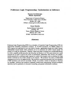
Figure 3-2: Energy vs. simulated delay and normalized logical-effort delay, the difference between the two graphs is the slope-correction term.
25
Comparing against simulation results Dsim, we can extract (3.5) by setting DLE,SC = Dsim − Derr,ref. The slope-correction term in (3.5) can be extracted as DSC = Dsim − Derr,ref – DLE. It is shown graphically in Figure 3-2, where Dsim is plotted against DLE + Derr,ref, and DSC is the difference between the two plots. From the slope-correction term, we can extract K of the gate, because gN·hN and gin-driverhin-driver are both known. For each gate, the extracted K varies slightly with fan-out due to the non-linearity of delay (Fig. 2-1), so K is determined as the least-squares fit of values extracted at different fan-outs. Even though this leastsquared fit provides a more accurate fit for K, it is more time consuming. To save time, we can instead perform simulation for only one typical scenario (i.e. delay slack of 10%), and the extracted K is generally within 5% comparing to the least-squares-fitted K.
3.4
Extracting K under VDD Scaling
As discussed in Chapter I, VDD scaling is very effective in reducing the energy dissipation for low-power applications, therefore, it is interesting to extract K under different supply voltages and observe any changes. Fortunately, supply voltage directly affects the drivecurrent of all gates, therefore VDD scaling only scales 0, and remaining logical effort parameters still provides an accurate linear fit. Given such scenario, we can simply gather the simulation data at different supply voltages, divide the delay by 0, and use (3.5) to re-extract K using the same method. The extracted K for a variety of gates are shown in Figure 3-3, under supply voltages of 0.5 to 1.2V. The inputs to NAND and NOR gates all provide similar K values, and are not plotted individually, but the inputs for the two branches in AOI are shown separately.
26
Slope correction factor, K
6
5
AOI12 NAND AOI12 NOR NAND3 NAND2 NOR2 Inverter
4 3
2 0.6
0.8 1 Supply Voltage, VDD (V)
1.2
Figure 3-3: Slope-correction factor K for different gates in a 65-nm technology across supply voltage of 0.5V to 1.2V. It is interesting to see that K reduces as supply voltage is decreased, suggesting a stronger input-slope effect. Intuitively, this is because drive-current is still exponentially proportional to gate-to-source voltage when the transistor is in sub-threshold. As VDD scales down, the transition point (VM) becomes very close to (and eventually crosses) VT. As a result of VDD scaling, the transistor that is turning on remains in sub-threshold for the majority (if not all) of its transition period, and because its drive-current is exponentially proportional to its gate voltage, a slow transition at its gate causes a larger penalty on delay. Therefore, gates operating in lower VDD are more sensitive to the inputslope effect.
27
In the end of Chapter II, we hypothesized that more complex gates will have larger values of K, because their limited drive-strength causes slow output transition long after the input has settled, making sizing a more dominant factor on their delays than input transition time. Such hypothesis is verified in Figure 3-2, where we see that complex gates such as AOI and NAND3 have larger values of K, while the inverter has the smallest value of K.
28
CHAPTER IV
Sizing Comparisons for Buffer Chains
4.1
Gate Sizing using Slope Correction Model
With the logical effort parameters and parameter K extracted (Chapter III), we can again use fmincon in Matlab to minimize gate sizes, but instead use the delay model (3.4) to serve as the delay constraint. However, it is interesting to note that the minimum delay possible with (3.4) is no longer produced by equal fan-out per stage. To validate this observation, let us examine the gradient differences between the two models. Using the logical effort model to estimate buffer chain delays, a N-stage buffer chain from (3.3) can be described as a function of gate sizes
C DLE gi i 1 pi Ci i 1 , N
(4.1)
where C1 = 1 and CN+1 = CLoad. Differentiating (4.1) and setting the derivative equal to 0, we obtain
0
C dDLE 1 gi 1 gi i 21 dCi Ci 1 Ci ,
and after multiplying both sides by Ci, we obtain
29
(4.2)
gi
Ci 1 C gi 1 i , Ci Ci 1
(4.3)
which means minimum delay is achieved by equal fan-out per stage, as expected from [2, 3]. However, equation (3.4) poses a slightly different scenario, because now there is a slope-correction term that is also a function of Ci. For easier differentiation, let us first formulate (3.4) as
C 1 C 1 DLE ,SC 1 gi i 1 pi gi 1 i Ki Ci Ki Ci 1 . i 1 N
(4.4)
Differentiating (4.4) and setting it equal to 0, we obtain
0
dDLE , SC
(4.5)
dCi
1 1 1 1 g 1 i 1 Ci 1 Ki Ki 1
Ci 1 1 C 1 1 gi 1 gi i 21 gi 2 Ci Ki Ci 1 Ki 1 Ci .
However, for the last stage driving the large capacitive load, there is no i+1th buffer stage, therefore the derivative of (4.4) for the last buffer stage (i = N) becomes
0
dDLE , SC
(4.6)
dCN
CLoad 1 1 1 1 1 1 1 g N 1 g N 1 gN 2 CN 1 K N CN KN CN 1 . K N 1 After multiplying both sides of (4.5) and (4.6) by Ci, we obtain
30
1 1 1 Ki 1 Ki
Ci Ci 1 1 1 1 gi 1 gi Ci 1 Ki Ki 1 Ci
1 1 KN
CLoad gN CN (when i = N).
(4.7)
Since every gate in a buffer chain is of the same gate type, parameter K is the same for every stage. This implies that every stage in the buffer chain will have the same fan-out, with the exception of the last stage: the fan-out of the last stage will be (1 – 1/KN) times larger than the previous stages. Using this formulation, the optimal fan-out per stage for the first N-1 stages are:
1 C FO N 1 load , K Cinput
(4.8)
and the fan-out of the last stage is FO·(1 – 1/K). Since the slope-correction model subtracts delay for tapered gates, this derivation suggests that the tapered scenario actually leads to a shorter minimum delay than that possible with the equal fan-out case.
4.2
Comparisons in the Energy-Delay Space
To characterize the differences between the original logical model and the slope correction model for low power designs, it is interesting to observe the estimation differences between the two models on the energy-delay space. Function fmincon is used to minimize the gate sizes given either (3.3) or (3.4) as the delay constraint, and the estimation results are compared against simulation.
31
In the previous chapter, Figure 3-2 plotted the differences between the logical effort model and simulation for NAND2 gate in 65-nm technology. The same gate is plotted in Figure 4-1 with both the original and the slope-corrected model shown. The reference error (Derr,ref) is subtracted from both models to isolate the error caused by tapering. As a result, all the plots start at internal energy of 1 and delay increment of 0, which is normalized to the equal fan-out case that is serving as the reference. We see the slope correction model provides a much more accurate delay estimation. Even for delay increment of 40%, where fan-out can reach 16 or more, the slope correction model is
Internal Energy (normalized)
only slightly more conservative.
Internal Energy (normalized)
1 0.8 Min Delay 0.6
0.4 0.2 0 -10
1
A B’
B
0.8 C
C’
D
0.6
D’ E
-1 0 1 Delay Increment (%)
Simulation Original LE LE with Slope Corr
0
10 20 30 Delay Increment (%)
40
50
Figure 4-1: Internal energy vs. delay curve for a NAND2 based buffer chain in a 65nm technology at 1V supply voltage.
32
From the inset in Figure 4-1, it is noticeable that tapering does lead to slightly lower delay comparing to the equal fan-out case. During initial downsizing (point A→B→C), delay actually decreases by nearly 1% (up to 3% under 0.5V supply) and then increases with further downsizing. By taking advantage of tapering, we can reduce energy and delay compared to the equal fan-out reference case. This advantage allows the tapered design to achieve the same delay as the reference case (point E) with 40% reduction in internal energy (varies from 25-60% depending on the type of logic gate and supply). The original logical effort model is inaccurate under tapering, leading to sub-optimal energydelay. For example, at 10% delay increment, the slope-correction model requires an internal energy of 0.28, while the original model requires 0.4. The minimum-delay point (point C) obtained by tapering cannot be predicted by the logical effort model (point C’), but the slope-correction model is able to locate the minimum delay (C) and construct an accurate delay estimation from that point on (C→D→E etc.). The slope-correction error is within 5% across all supply voltages when the fan-out is less than 32, which is the case in most applications. However, the error may reach 15% for fan-outs greater than 80, because it is difficult to model such large fan-out with this linear model. To demonstrate the scenario under different supply voltages, Figure 4-2 shows an inverter chain in 65-nm technology at VDD of 1.0V and 0.5V. We see the energy-delay characteristics of the inverter at 1.0V is very similar to that of the NAND2 case, actually most logic gates operating at 1.0V have similar energy-delay curves.
33
1
Simulation 0.9
Original LE LE with Slope Corr
Internal Energy (normalized)
0.8 0.7 0.6 0.5 0.4 0.3 0.2 0.1 -10
0
10
20
30
40
50
Delay Increment (%)
a) 1
Simulation 0.9
Original LE LE with Slope Corr
Internal Energy (normalized)
0.8 0.7 0.6 0.5 0.4 0.3 0.2 0.1 -10
0
10
20
30
40
50
Delay Increment (%)
b) Figure 4-2: Internal energy vs. delay curve for an inverter chain in a 65-nm technology at (a) 1V supply voltage (b) 0.5V supply voltage.
34
Under the low VDD of 0.5V, however, the energy-delay curve is sharper – the “knee” is much more apparent. The original logical effort model still provides the same estimation curve as the 1.0V case, but the slope correction model (with a different K for 0.5V) models very accurately. We see that 70% of internal energy can be achieved without sacrificing delay at 0.5V, but such significant advantage of tapering is not modeled by the original logical effort model.
4.3
Limiting Factors in Sizing Effectiveness
In this chapter, we observed that sizing is an excellent optimization in reducing the internal energy of an equal-fan-out datapath. However, its effectiveness greatly diminishes after ~20% delay increment, and additional delay slack produces very little energy savings. Plus, most commercial designs have an upper limit on fan-out and transition time due to reliability concerns, which puts an additional boundary on tapering. If the upper-bound on fan-out is 16, then the previous designs could not have internal energy of less than 0.2, which means tapering is only effective up to about 20% of delay slack. In addition, tapering gate sizes only reduces the internal energy of the buffers, and not the total energy. For buffers driving a large load, reducing the internal energy quickly reaches diminishing returns. For the case in Figure 4-2b), even though 20% delay slack can reduce internal to merely 15% comparing to the reference case, the internal energy at that point is only about 3% of the total switching energy. To further reduce
35
energy for low power designs, it is essential to also reduce the energy in the load. Due to the necessity to allow more energy reduction than sizing alone, and to reduce the total (and not internal) energy, we ought to incorporate supply voltage reduction in our optimizations. We see in the next chapter that reducing VDD can take advantage of a larger delay slack to allow more energy reduction, and reduces the total energy of the design as well.
36
CHAPTER V
Incorporating Supply Voltage Optimizations
5.1
Modeling Delay under Supply Voltage Scaling
In the previous chapter, we observed that sizing is only effective up to around 20% delay slack, and it only reduces the internal energy of the gates, but not the energy in charging and discharging the load capacitance. To address such issues, it is evident that supply voltage reduction is necessary for low-power designs. It does lead to exponential increase in energy as VDD approaches VT, but such technique allows much more energy reduction than sizing alone. To incorporate supply voltage optimization, it is necessary to accurately model gate delay as a function of VDD. Recent short-channel technologies can be well-modeled by the alpha-power model introduced in [15], where drive-current of a transistor is modeled as
I D A VDD VT ,
(5.1)
where parameters A, VT, and α are fitted for each technology. Given such formulation, we can then model the gate delay as
tp
C VDD VDD . I VDD VTH
37
(5.2)
Extracting the required parameters is not difficult: given an equal fan-out buffer chain, we can simply gather its delay VDD is scaled down. Using the delay at 1V as reference, we can model the delay ratio as
Delay Ratio (VDD )
VDD (1 VT ) , (VDD VT ) 1
(5.3)
and a least-squared-fit should be able to extract parameters VT and α. The above formulation should model delay accurately for the equal fan-out case, as long as the transistors are operating in strong-inversion (moderate- and weakinversions will be discussed later). However, for the tapered scenario, using a fixed K is insufficient to model all supply voltages, for we observed a lower K under lower VDD (Figure 3-2). Similar to the alpha-power model, we can model K as
K VDD
V V A DD TH VDD
K ref
,
(5.4)
Where parameters A, β, and Kref are obtained by least-squares curve fit of the extracted K in Figure 3-2. Since K is in the denominator of the slope correction model, K(VDD) is essentially an inverse of (5.1) with a constant Kref added for improved model accuracy. Adding Kref also prevents K from reaching 0 as VDD scales down to VT (as in subthreshold operations), for a K of 0 suggests (unrealistic) infinite slope-correction. For the inverter chain in a 90-nm technology, we obtained A = 1.3, = 1.4, and Kref = 1.62. The modeled K function fits very well against the extracted K values from Figure 3-2.
38
5.2
Concurrent Optimization of Sizing and Supply Voltage
With models for both delay ratio and parameter K as a function of VDD, we can revisit the 5-stage buffer chain example from the previous chapter, but this time optimizing for both sizing and supply voltage concurrently using the fmincon function in Matlab. The nominal voltage is 1.0V, and since supply voltage reduction is able to reduce the total (and not just internal) energy of the datapath, total energy and VDD is plotted against delay in Figure 5-1. In the previous chapters we demonstrated sizing to be very effective during initial energy reduction of minimum-delay designs, such scenario still holds true here. We see from Figure 5-1 that VDD remains at 1.0V during the first few percentages of delay increase, but give more delay slack, supply voltage reduction becomes the dominant optimization variable for the majority of lower-power optimizations. Such scenario can also be observed visually, where the shape of the majority of the energy-delay curve seems to be a mere quadratic function of the VDD-delay curve. Supply voltage scaling, however, also comes at a cost in performance. We see in Figure 5-1 that a 63% reduction in total energy comes at a 100% increase in path delay, and the energy-delay curve is flattening out, suggesting more delay penalty would apply under further VDD reduction. Nevertheless, it is interesting to observe the maximum potential energy savings achievable with supply voltage scaling. However, it is evident that such optimization is pushing VDD towards VT, which causes the alpha-power model from (5.1) to approach 0 (and the delay to approach infinity). Given such inaccuracies, we must first establish an accurate current and delay model for the near- and sub-
39
threshold region to be able to effectively optimize low-power circuits under such regions
Total Energy (normalized)
of operations.
Total Energy (normalized)
1 0.9 0.8 0.7 0.6
1 0.9 0.8 -2 0 2 4 6 Delay Increment (%)
0.5 Simulation Original LE LE with Slope Corr
0.4 0.3
0
20
40 60 Delay Increment (%)
80
100
80
100
a) 1 0.95
VDD
0.9 0.85 0.8 0.75 0.7 0.65 0
20
40
60
Delay Increment (%)
b) Figure 5-1: Total energy (a) and VDD (b) vs. delay for an inverter chain in 90-nm technology.
40
5.3
Sub-threshold and IC Model
As supply voltage reaches threshold voltage, it is generally acceptable to model both onand off- currents of a transistor using the sub-threshold leakage equation:
I ON I Leakage e I Leakage I S e
VDD nt
VDD VT nt
I S 2 n Cox
,
(5.5)
, and
(5.6)
W 2 t L ,
(5.7)
where n is the sub-threshold slope factor, σ is the DIBL factor, and Φt is the thermal voltage given by kT/q, or 26mV at room temperature. Mobility and oxide capacitance Cox are the same as those from traditional I-V equations. Such model is able to model sub-threshold current quite accurately; however, we will see that this model is not suitable for optimizing VDD for low-power designs. As shown in Figure 5-2, the α-power model is unable to model current as VDD approaches VT, and the leakage model becomes inaccurate once VDD reaches above VT. However, in the moderate inversion regime, where VDD is close to VT, neither model is able to model the on-current very accurately. This issue is non-trivial, because we will see that the moderate-inversion regime is very attractive for low-power designs. Another issues that arises with combining α-power and leakage model is that the ID(VDD) function is not continuous at the transition point. Although we can modify the fitting parameters to make the two equations equal at the transition point, this comes at a
41
6
10
4
10
ID (nA)
Vth 2
10
0
10
simulation -power model leakage model
-2
10
0.1
0.2
0.3
0.4
0.5 0.6 VDD (V)
0.7
0.8
0.9
Figure 5-2: VDD vs. ID for α-power and leakage model against simulation. cost of modeling accuracy for the rest of the VDD regimes. Such forced-fitting of the parameters still do not guarantee the gradient of the two functions to be continuous at the transition point, which may cause difficulties during optimizations. Even if the two gradients cannot be equal at the transition point, the gradient of the α-power model should be steeper than the leakage model at the transition to preserve the convexity of the ID(VDD) function. Fortunately, extensive research has been conducted in such area, and an IC/EKV model has been developed in [16] that is accurate for all regions of transistor operation. IC represents the inversion coefficient, which is around 1 for VDD = VT (moderate inversion), much less than 1 for sub-threshold operations (weak inversion), and reaches
42
around 100 for strong inversion. The on-current of a transistor can be modeled as:
I ON
IC I S , k fit
(5.8)
1 VDD VT 2nt IC ln e 1
2
,
(5.9)
where kfit is a fitting factor, and the remaining parameters are the same as those in (5.6). 6
10
4
10
ID (nA)
Vth 2
10
0
simulation -power model leakage model IC model
10
-2
10
0.1
0.2
0.3
0.4
0.5 0.6 VDD (V)
0.7
0.8
0.9
Figure 5-3: VDD vs. ID for α-power, leakage, and IC model against simulation. Even though the IC model is not as intuitive as the α-power and the sub-threshold model, and is generally not used for hand-calculations, it is attractive for optimizations because it accurately models the on-current under all regions of VDD (Figure 5-3).
43
4
10
simulation IC+leakage model
3
Ion and I leakage (nA)
10
2
10
MSEIC = 0.18% 1
10
0
10
MSEleakage = 0.21% -1
10
-2
10
0.1
0.15
0.2
0.25
0.3 VDD
0.35
0.4
0.45
0.5
1
10
ICIC= =1 1atat0.372V 0.372
0
10
-1
Fitting parameters:
IC
10
IS = 0.9934 μA σ = 0.1255 VT = 0. 3798 V n = 1.3819 kfit = 1.2678
-2
10
-3
10
-4
10
0.1
0.15
0.2
0.25
0.3
0.35
0.4
0.45
0.5
VDD
Figure 5-4: VDD vs. Ion and Ioff for the IC model against simulation. The off-current is still modeled by the leakage model from (5.6), and given the same set of parameters, the fitting accuracy for both the on- and off- current are within 0.2% mean-squared-error. The simulated and fitted plots for on- and off- current, along with
44
IC, are shown in Figure 5-4. The same set of fitting parameters is used for both on- and off- currents. We see the point where IC=1 is slightly lower than VT. However, it is generally desirable to have IC=1 correspond to VDD = VT, which draws a clear boundary between strong and weak inversion regimes. When VDD = VT, the following equation holds true:
VT (1 ) VT 2 n t ln e
IC
.
1
(5.10)
By set IC = 1 under such equation, we can set parameter n to be:
n
VT
2 t ln e 1 .
(5.11)
By removing one fitting variable, means-squared-error of the fit has increased from 0.2% to 0.4%, but is more than sufficient for our optimization purposes. From the IC model, it is evident that VT plays an important role in supply-voltage optimization, for it is generally the difference between VDD and VT that determines the delay ratio, and VT also plays a critical role in determining the leakage current. It is therefore desirable to optimize VT concurrently with VDD; however, such approach is generally not feasible in modern-day CMOS processes, as the VT is generally fixed for the given technology. However, most processes offer at least two different threshold voltages for the same technology, therefore it is interesting to compare the on-/offcurrent and fitting differences between high-VT (HVT) and low-VT (LVT) cells. We aimed to have a single set of fitting parameters for both types of transistors, which has increased the mean-squared error form 0.5 to 1.5%, but is still very reasonable. The plots for on- and off- current, along with IC, are plotted against VDD in Figure 5-5.
45
10
Current (nA)
10
10
6
4
Fitting parameters:
HVT
2
I
IS = 0.998 μA σ = 0.105 VTL = 0.376 V VTH = 0.519 V n = 1.410 kfit = 1.406
on
LVT 10
10
10
0
HVT
I
-2
leakage
LVT
-4
10
10
IC
simulation model
10
10
10
0.1
0.2
0.3 V
DD
0.4 (V)
0.5
0.6
2
0
V -2
V
T,LVT
T,HVT
LVT
HVT
-4
-6
0.1
0.2
0.3 V
DD
0.4 (V)
0.5
0.6
Figure 5-5: VDD vs. Ion and Ioff for the IC model for LVT and HVT cells.
46
5.4
Modeling Energy under Supply Voltage Scaling
In the previous chapters, sizing is the main optimization goal, and energy is simply modeled to be linearly proportional to sizing. Such assumption holds true for sizing optimizations alone, for sizing is linearly proportional to both switching (CL=W·Cox) and leakage (IS=W·IS0) energy. Under VDD scaling, however, the relationship between energy and VDD is much more complex. Though VDD is quadratically proportional to switching energy, such case is not true for leakage energy. In addition, leakage energy-peroperation is dependent on the speed of the operation, for a slower design also spends more time consuming leakage. Under sizing optimization alone, a fast design with less than 20% increase in delay does not affect leakage by a significant amount, but when delay is increased by 100-1000× under aggressive VDD scaling, this exponential increase in delay eventually leads to an exponential increase in leakage energy. The energy-per-operation of a datapath can be modeled as the sum of switching and leakage energy, 2 EOP esw elk CL VDD
D
I leakage VDD
.
(5.12)
The formulation for elk is quite interesting, for it is a product of leakage power (Ileakage·VDD) with the time duration of leakage, D/α. Parameter α here is the activityfactor (not to be confused with the α-power model), which defines the number of active (switching) clock-cycles per total clock-cycle. For most datapaths, α varies from 0.1% to 10%. Parameter D is the clock period, which is determined by the critical-path delay of the datapath. Given the formulation in (5.12), the energy-per-operation of a datapath with
47
1% activity factor is the sum of its switching-energy and its leakage-energy over 100 clock cycles. Evidently, low-activity datapaths are energy-inefficient, for they are required to idle for longer periods of time before a useful operation is performed. Expanding (5.12) and isolating gate sizes from VDD, we can express the energy-peroperation as VDD VT D W0 2 nt 2 EOP Wi Cox VDD 2 n Cox t e VDD . L i 1 n
(5.13)
5.5
Optimization with Aggressive Supply Voltage Scaling
With an accurate delay and energy model for all regions of transistor operation, we can now explore the energy-delay optimization space for very low-power designs, where VDD is aggressively scaled down to VT or below. As stated in previous sections, leakage energy per-operation will increase under aggressive VDD scaling due to the exponential increase in delay causing parameter D in (5.13) to increase. The point of minimum energy (MEP) is reached when the increase leakage energy under further VDD reduction equals the additional reduction in switching energy. The exact location of MEP depends on many factors, but the threshold voltage and the activity factor of the design plays a dominant role. Figure 5-6 shows two designs, with different activity factors and threshold voltage, near their respective points of minimum energy.
48
4 E 3.5
E
LVT = 1%
LVT = 1%
sw
E LVT = 1%
3
Energy (norm. to MEP)
total
lk
2.5 2 1.5
MEP 1 0.5 0 1
2
10
10
Delay (norm. to MDP)
a) E 2 E
total sw
HVT = 10%
HVT = 10%
E HVT = 10% lk
Energy (norm. to MEP)
1.5
MEP 1
0.5
0 3
4
10
10 Delay (norm. to MDP)
b) Figure 5-6: Total, switching, and leakage energy vs. delay for (a) LVT with α=1% and (b) HVT with α=10% designs.
49
As expected, the LVT design in Figure 5-6 a) suffer from more leakage due to its lower threshold voltage and lower activity factor. As a result, MEP occurs around VDD of 0.355, slightly below VT of 0.376, and the total energy reduction is 13.9× lower than that of minimum-delay point (MDP). In comparison, the design in b) is much more immune to leakage due to its higher activity factor and higher VT. As a result, MEP occurs around VDD of 0.236, much lower than its VT of 0.519, and the total energy reduction is 31.2× lower than that of MDP. The large energy savings from MEP-operation seems very attractive, but such savings comes at a large penalty in performance. For the design in Figure 5-6 b), MEP costs more than 30000× in performance comparing to the minimum delay point. Fortunately, near-MEP operation can often benefit from a large increase in performance with little cost in energy (in contrast to minimum-delay optimizations). It is therefore interesting to observe the effectiveness of different optimization parameters to reduce delay near MEP. Unlike energy-delay optimizations near MDP, where we are interested in the optimization variable that provides the most energy-reduction per cost in delay, we are now interested in the variable that provides the smallest energy-increment per reduction in delay. Figure 5-7 and 5-8 demonstrates the effectiveness of sizing and VDD (jointly and individually) when optimizing a LVT design from MEP. It is apparent that sizing is not effective near MEP, for their cost in energy is much larger than that for VDD scaling. As a result, the energy-delay optimization is virtually driven by VDD optimization alone, until near MDP where sizing began to take effect when VDD has reached its upper bound. It is
50
also apparent that a lower activity factor is detrimental in respect to energy-per-operation.
opt(V
,W ), = 10%
DD
i
= 10%)
opt(W ) only, = 10% i
opt(V opt(V
1
10
) only, = 10%
DD
,W ), = 1%
DD
i
Energy (norm. to MEP for
opt(W ) only, = 1% i
opt(V
) only, = 1%
DD
0
10
0
10
1
2
10
3
10
10
Delay (norm. to MDP)
Figure 5-7: Energy vs. delay for sizing and VDD optimizations with α = 1% and 10%. 1
= 10% = 1%
0.9
0.8
Vdd (V)
0.7
0.6
0.5
VT
0.4
0.3
0.2 0 10
10
1
10
2
10
3
Delay (norm . to M DP)
Figure 5-8: VDD vs. delay for the VDD optimization above.
51
To have a closer view of the effectiveness of sizing, VDD, and (when possible) VT in the energy-delay space, let us examine the energy-delay sensitivities of the individual variables, shown in Figure 5-9.
Sensitivity
10 10 10 10 10 10
3
100 S(W i)
0
S(VDD) S(VT)
-3
10
-6
-9
-12
Energy (norm. to MEP)
10
1 -15
10
0
10
1
2
3
4
10 10 10 Delay (norm. to MDP)
10
5
Figure 5-9: Energy-delay sensitivity (left-axis) and energy-delay tradeoff (rightaxis). 10
1
10
-4
S(W ) i
S(V
10
10
0
DD
)
10
-6
S(VT)
Sensitivity
Sensitivity
10
-1
10
10
-8
-10
Sens(Wi)
-2
10
-12
Sens(VDD) Sens(V ) T
10
-3
1
1.2 1.4 1.6 Delay (norm. to MDP)
10
1.8
-14
1.8
1.6 1.4 1.2 Energy (norm. to MEP)
Figure 5-10: Energy-delay sensitivity near MDP (left) and MEP (right).
52
1
Figure 5-9 shows simulated energy-delay sensitivity for an adder as well as optimal E-D tradeoff. Figure 5-10 shows a detailed zoom of areas around MDP (left) and MEP (right) to compare techniques for high-performance and low-power design optimization. For the optimal E-D curve, the sensitivities of the active parameters need to be equal. For highperformance optimizations, we aim for the variable with the highest sensitivity (for largest energy reduction given delay increment), so when the sensitivity curve of a parameter deviates from the highest curve, such parameter has reached its constraint limit, and is no longer active to support further energy reduction.
For low-power
optimizations, we aim for the variable with the lowest sensitivity (for smallest energy penalty given delay reduction), so when the sensitivity curve of a parameter deviates from the lowest curve, such parameter has reached its constraint limit, and is no longer active to support further delay reduction. This is the case with VT and sizing at MEP, and VT and VDD at MDP. As expected, near MEP, VDD tuning has the lowest sensitivity (it has least increase in energy for a given delay reduction), and thus the most effective parameter in delay reduction. As we traverse up the E-D curve, VT tuning also becomes a significant parameter, and sizing becomes a significant parameter only under high VDD and low VT scenarios, (Figure 5-10, left), where we require high-performance designs. From the sensitivity analysis in Figure 5-9 and 5-10, it is interesting to see that VT is an active constraint throughout most of the energy-delay space. It is more effective than VDD scaling in the high-performance regime, and more effective than sizing in the low-power regime. Although VT is not easily varied in the device level, recent research such as [18] is able to vary VT using novel circuit topologies. Nevertheless, it is
53
interesting to compare the energy-delay space achievable when VT is incorporated as an optimization parameter. The optimization results are shown in Figure 5-11 and 5-12. Var-VT
= 0.1% = 10%
Energy (fJ)
LVT 10
1
HVT
10
0
10
Var-VT -1
10
0
HVT
LVT
10
1
2
3
4
10 10 10 Delay (ns) Figure 5-11: Energy vs. delay for adder optimization through VT adjustment.
1 VDD VT
Voltage (V)
0.8 = 0.1%
0.6
0.4 = 10%
0.2
0 -1 10
10
0
10
1
2
3
4
10 10 10 Delay (ns) Figure 5-12: VDD vs. delay for adder optimization with VT as an optimization variable.
54
Given the freedom to vary VT, we can achieve equal or higher energy-delay efficiency than any fixed-VT cells across all regions of the energy-delay space, and for all activity factors. For the lower activity factor of 0.1%, varying VT can achieve similar energy efficiency as the HVT cells for very low power regimes while preserving the advantage of LVT cells in other regimes. For the higher activity factor of 10%, varying VT gives a clear advantage in the energy-delay space. It is evident that low activity factors are less energy efficient. This is because designs with low activity are more affected by leakage, which increases exponentially under supply voltage reduction. To obtain higher energy efficiency, it is beneficial to perform architectural optimizations to minimize the cost of leakage. For high-performance designs, however, energy is dominated by switching energy, so activity factor plays a less significant role. Since architectural changes are separate from circuit optimizations, it will be discussed in the appendix chapter. From Figure 5-11, it is evident that although HVT cells could achieve lower energy-per-operation than LVT, they carry a 10-100× performance penalty comparing to LVT cells. Such high performance penalty for marginal energy reduction is highly undesirable in low-power design. For performance-constrained low-power designs, it is generally more effective to use LVT cells and operate at a lower VDD than using HVT cells, which would require a higher VDD to meet the same performance.
55
CHAPTER VI
Optimization for Synthesized Design
6.1
Low Power Optimization for Synthesis Flow - Issues
Having discussed the theoretical aspects of energy-delay optimization with respect to different optimization parameters, it is beneficial to apply the discussed techniques to more real-life designs. Design optimization of individual buffer chains and datapaths, which were given as an example in previous chapters, are seldom used in real-life design practices. Although they served as good demonstrations in providing design insights, it is nevertheless necessary to apply such techniques to logic synthesis, which is the design approach for the vast majority of modern-day logic designs. Logic synthesis and place-and-route has enabled design and implementation of very high-complexity circuits in a timeframe that would have not been possible for fullcustom designs. In the silicon industry, where time-to-market and design cost (in manhours) are critical to the success of a product, this automated-design-flow has become the integral part of the design tape-out for most companies. Unlike research-based designs, where state-of-the-art performance and power-numbers appears to be the utmost design criteria, the major criteria for commercial designs are long-term functionality and reliability, along with high manufacturing yield. Performance and power are only optimized given these major criteria are not violated. As transistor scaling continues, the
56
pressing issue of reliability and yield has led to greater manufacturing difficulties in the fabrication process, ever-more-stringent design rules for the physical-design flow, and is affecting logic design as well. The previous chapters have established that increasing fan-out towards the latter stages is a common result of tapering for low-power designs. However, reliability issues with electro-migration and hot-carrier-effects have placed a strict limit on transition time [19]. Since transition time is directly correlated to fan-out, the maximum fan-out of most designs is limited to 8-16. This constraint has some effects on the limits of tapering, but as shown in chapters IV and V, sizing does not contribute to significant energy reduction after 20-30% delay increment, so allowing excess fan-out (at the cost of reliability) does not contribute much to additional energy savings. We see in the previous chapter that the dominant optimization parameter for low-power design is VDD scaling. In modern day CMOS, however, low VDD operation near the minimum-energy point is still very rare in commercial designs, mostly due to the increased penalty of process variability under low VDD. As VDD scales down towards VT, we observe a near-exponential increase in delay, because transistor current in near- and sub- threshold are exponentially proportional to (VDD - VT). However, due to the nature of the manufacturing process, the silicon bodydoping cannot be precisely controlled [20], therefore it is common to observe 50-100mV of threshold voltage variations even from the same wafer. Such variation in VT may cause more than 30% timing differences under a nominal VDD of 1-1.2V, but could easily lead to timing failures when the operational VDD is only 100mV above VT. Such VT variation
57
also causes 10× variations in leakage, but for most commercial designs, the penalty of timing failure is much more severe than the penalty of a less power-efficient chip. To target the increased effect of process variations on low VDD designs, some have used back-gating (body-biasing) for fine-tuning VT after fabrication [21, 22], but the implementation overhead in fabrication (triple-well process) and chip-characterization is non-trivial. In other cases, some state-of-the-art synthesis libraries are providing not only the timing information (.lib file) for nominal voltages, but for an entire range of V DD for all process corners (mainly typical-NMOS-typical-PMOS (TT), slow-NMOS-slowPMOS (SS), and fast-NMOS-fast-PMOS (FF) cases; some provides slow-NMOS-fastPMOS (SF), and fast-NMOS-slow-PMOS (FS) information as well). However, characterizing such timing information for all standard-cells within a design kit is a nontrivial task, so most synthesis libraries that we have encountered only includes the .lib timing information for the nominal VDD (1-1.2V). As a result, it is essential to properly characterize the low-VDD performance variations of a given process technology.
6.2
Characterizing Low-VDD Performance Variations
From the previous chapter, we see that near-MEP operation generally does not occur below 0.3V for our 65-nm technology. As a result, we need to characterize the timing differences between TT, SS, and FF corners for VDD down to 0.3V. The characterization is first performed on a fan-out 4 inverter, similar to the cases in Chapter III. As expected, the timing differences between the FF, TT, and SS corners are 30% under 1.0V VDD, but increased to 3× as VDD scales down to 0.3V.
58
Inverter Delay vs. V
3
DD
TT
3X
10
SS FF
t p , normalized to 1.0V-TT
3X 2
10
1
10
30% { 30% {
0
10
0.3
0.4
0.5
0.6
0.7
V
DD
0.8
0.9
1
(V)
Figure 6-1: Inverter delay (tp) vs. VDD, normalized to delay at 1.0V-TT corner. Due to such large discrepancy in delay under low VDD, it is essential that the delay-VDD relationship of the SS-corner is used for calculating synthesis timing constraints. For example, if the desired operating frequency is 1MHz under 0.4V V DD, and Figure 6-1 shows a 100× delay increase in TT-corner from 1.0V to 0.4V, but 250× delay increase in SS-corner, we must synthesize for 250MHz using the SS-timing library for 1.0V. However, characterizing delay-VDD for an inverter may not be sufficient, as [14] have suggested, complex gates with stacked PMOS and NMOS may behave differently from inverters in sub-threshold operation. One of the most sensitive stacked logic is a D-flip-flop, so we have also characterized the relationship between its clock-toq delay and VDD. Fortunately, the delay of the flip-flop scaled very similarly to that of an inverter, as shown in Figure 6-2.
59
Inverter and Flip-Flop Delay vs. V
DD
SS Inverter
3
10
SS Flip-Flop TT Inverter
t p , normalized to 1.0V-TT
TT Flip-Flop FF Inverter
2
10
FF Flip-Flop
1
10
0
10
0.3
0.4
0.5
0.6 V
0.7 DD
0.8
0.9
1
(V)
Figure 6-2: Inverter delay and clock-to-q delay vs. VDD, normalized to inverter and clock-to-q delays at 1.0V-TT corner. However, having a design that meets timing in SS corner may not be sufficient. In modern day standard-cell libraries, the PMOS is generally sized to have small drivecurrent than NMOS. This creates shorter average rise/fall delays than upsizing the PMOS to have equal drive strength. Under very low VDD, however, the weaker drive-strength of the PMOS gate may result in insufficient on-current to over-power the leakage current of its NMOS counterpart. As a result, complex gates with stacked PMOS are the most likely to create failures, especially in the FS (fast-NMOS-slow-PMOS) corner [14]. The following two transient responses demonstrate the above scenario. Figure 6-3 shows the SS corner clock-to-q delay of a D-flip-flop under a VDD of 150mV. We see the clock-to-q delays are both in the microsecond range, with an average clock-to-q delay of
60
clk-to-qfall
clk-to-qrise
Figure 6-3: The clock-to-q transition of a D-flip-flop under 150mV SS corner.
Fail
Figure 6-4: The clock-to-q failure of a D-flip-flop under 165mV FS corner.
61
6.93 us. Such long delay is not suitable for most applications, and a supply voltage of 150mV is well below the optimal VDD for minimum energy (given this 65-nm process). Realistically, this scenario will not occur in a well-optimized design, but nevertheless the flip-flop is fully functional in the 150mV SS corner. Figure 6-4 shows the FS corner of the same flip-flop under a VDD of 165mV. Even though the supply voltage only increased by 15mV, we already observe much sharper clock transitions comparing to the 150mV case, and the NMOS transitions are much faster than PMOS as expected. However, the flip-flop is unable to function properly in this scenario. We see the data transition pulledup properly after the second positive-clock-edge, but after the clock (and input data, not shown) turned low, the flip-flop is unable to hold its value until the next positive clockedge, and produced an early data transition. Fortunately, such scenario does not occur above 0.2V for this 65-nm technology, which is lower than the E-min VDD of 0.3V, therefore using the SS model for worst-case timing characterization is sufficient
6.3
Standard-Cell Designs and the Slope Correction Model
It is previously shown that the slope correction model is able to optimize the sizing of full-custom designs, but to use this model for standard-cell logic, a few changes are needed. Most standard-cell logic are synthesized by a synthesis tool, so they are generally in a “netlist” format, where the instantiations of each cell and its input/output connections are specified in a text file. For the Matlab environment to understand the gate instantiations and connections, some netlist-reformatting are required (Figure 6-5).
62
INVX8 g2653(.A (n_294), .Y (Z[15])); INVX8 g2657(.A (n_291), .Y (Z[13])); INVX6 g2655(.A (n_292), .Y (Z[14])); NOR2X4 g2654(.A (n_282), .B (n_277), .Y (n_294)); INVX8 g2665(.A (n_289), .Y (Z[11])); NOR2X4 g2656(.A (n_287), .B (n_280), .Y (n_292)); NOR2X4 g2658(.A (n_283), .B (n_281), .Y (n_291)); INVX12 g2679(.A (n_286), .Y (Z[9])); NOR2X4 g2666(.A (n_278), .B (n_267), .Y (n_289)); AOI21X1 g2833(.A0 (n_49), .A1 (n_50), .B0 (n_65), .Y (n_124)); ...
IV IV IV NOR IV NOR NOR IV NOR AOI
1 1 1 2 1 2 2 1 2 2
8 8 6 4 8 4 4 12 4 1
g2653 g2657 g2655 g2654 g2665 g2656 g2658 g2679 g2666 g2833
n_294 n_291 n_292 n_282 n_289 n_287 n_283 n_286 n_278 n_49
n_277 n_280 n_281 n_267 n_50
n_65
Z[15] Z[13] Z[14] n_294 Z[11] n_292 n_291 Z[9] n_289 n_124
Figure 6-5: The original netlist in text and the reformatted netlist in Excel. The process of re-formatting may seem tedious, but it is quite straightforward using search-and-replace functions. The “tabs” in text are automatically translated as a new column in excel, so the important parameters in the text file (gate type, size, name, input/output wires, etc) can be automatically assigned to the correct column by adding tabs in between them. The data from the Excel spreadsheet (text and numbers) can then be imported into Matlab by the xlsread function. Instead of specifying the transistor width of each logic gate, the standard-cell library simply uses a number to represent the “gate size”. Depending on the type of the
63
gate and the technology library, the transistor width for a specific gate size may change (e.g. transistor sizes for INV2 in 90-nm are different from the INV2 in 65-nm technology, and the transistors sizes for NAND2 and INV2 are different, even though they both have drive-strength of 2). Since the choices for gate sizes are limited in the standard-cell library, delay and energy become discrete functions of gate sizes, similar to stepfunctions. The Matlab function fmincon (used in Chapter IV and V) is ineffective for step-functions because they are very discontinuous and contain many false local-minima (the gradient remains 0 between two gate sizes). We therefore need to use the function fminsearch for this optimization; unlike fmincon, it is a simplex search method that does not use numerical or analytic gradients, therefore it applies to non-continuous functions as well [23]. Before we use the slope correction model to optimize standard-cell designs, it is interesting to first evaluate the accuracy of timing library files against our logical effort models and simulation results. In the following sections, we first compare synthesis tool estimations and logical effort models for two synthesized adders. We then optimize the adders using the slope-correction model and compare the accuracy of these estimations at various energy-delay points.
6.4
Comparison of Estimation Accuracy
To perform a controlled comparison between the models and to isolate the timing errors due to tapering, two versions of a 16-bit parallel adder were synthesized using a 65-nm standard-cell library, both have about 16 logic stages with more than 300 gates. The first
64
version only drives 2fF load at each output, which equals its input capacitance. This acts as a reference case for the accuracy of the original logical effort model because there is very little tapering. There is actually negative tapering involved due to such small output capacitance, hence the original logical effort model estimates slightly shorter delays than the slope-correction model. The estimation errors are shown in Table 6-1. TABLE 6-1. DELAY COMPARISONS FOR TWO SYNTHESIZED ADDERS Delay Estimation Error %
Adder Designs
Original LE
Slope-Corr. LE
Synthesis Library
2fF load
4.3%
4.7%
11.2%
512fF load
41.6%
6.3%
9.7%
The second version is synthesized for minimum delay with 512fF load at each output. In this case, the original logical effort model greatly over-estimates the delay, especially in non-critical paths where the fan-out is 30 or more. Yet the slope-corrected model shows only 1.6% more error than the 2fF case. The synthesis estimation is conservative by about 10% in both cases, which is a good margin to reserve for the placeand-route flow. Knowing that the slope correction model maintains its accuracy for synthesized designs with multi-fan-out datapaths, we continue to perform sizing optimizations using this model.
65
6.5
Sizing Synthesized Design using the Slope Correction Model
To further demonstrate the slope-correction model on synthesized logic, we extended the optimization tool in Matlab to accommodate standard-cell based designs, as shown in Fig. 6-6. The tool first reads in the synthesized netlist and calculates the current criticalpath delay using the slope-correction model. Based on the circuit topology and standardcell library, the minimum achievable delay is determined (similar to Chapter IV). Such estimation may not be fully accurate, since it is determined by minimizing each individual path delay while assuming all branching fan-outs to be fixed. However, the estimation error is usually less than 1%. The user may then specify how much delay slack to allow; we have allowed 0-30% of slack to gather enough energy-delay information. Import netlist & create gate connections Determine minimum achievable delay Enter delay slack Initial critical path meets timing? Yes
No
Minimize energy of critical-path gates
Resize path to meet delay
Minimize energy of non-critical-path gates
Resize path to meet delay
Critical path meet timing?
No
Yes, exit Figure 6-6: Flow diagram of the optimization tool.
66
With the specified timing constraint, the Matlab tool locates the timing-critical paths and corrects the paths that violate timing; this process usually results in increased energy. After timing is met, gates in the critical and non-critical paths are optimized using similar methods as described in Chapter IV to minimize energy. Since the non-critical paths have more timing slack, the energy optimization tends to use smaller gates, which leads to a larger fan-out toward the output of the path. Without fan-out restrictions, it is possible to reach fan-out of up to 80 with this tool, where the delay estimation may have error up to 15%. However, such high fan-out errors only occur on non-critical paths, so the accuracy of the critical-path delay estimation is unaffected. If such large fan-out is not desired, the user may specify a maximum fan-out limit.
6.6
Comparison of Sizing Optimization Results
Using the design (Fig. 6-7, A) synthesized for minimum delay as a starting point, discrete sizing optimization is performed using the slope-correction model to obtain the new minimum delay (Fig. 6-7, B). From this point on, the adder was optimized by gate sizing using the slope-correction model. The optimization is done for 5 delay targets to meet delay slack up to 30%, each design corresponds to a data point on the energy vs. delay curves in Fig. 6-7. The delay estimated by the slope-correction model is compared against Spectre simulations, synthesis timing, and the logical effort model. The internal power is obtained by Spectre simulation.
Due to the limited sizing choices in the
standard-cell library, the energy vs. delay curve is not as smooth as those for buffer chains. However, we can still achieve more than 20% of internal power reduction over
67
the synthesized adder while maintaining the same delay. The average delay error in the slope-correction model is less than 5% compared to simulation, which is consistent with the reference error in Table 6-1.
50 A
Internal power (W)
45
Synthesized Adder
Simulation LE with Slope Corr Synthesis Timing Original LE Model
B
40 Matlab Optimized Adders
35
30 25 0.8
1 1.2 1.4 1.6 1.8 2 Delay (normalized to the synthesized adder)
Figure 6-7: Energy vs. delay for a 16-bit adder driving 512 fF of load, optimized with the slope-correction model using 65-nm standard-cell library. Gates in the non-critical paths are minimized in the optimization process, however, the synthesis timing library builds additional margin for these small gates. This led to more conservative timing estimations by the synthesis library; actual delays are shorter by up to 20%. The original logical-effort model has errors up to 40% compared to simulation, and is clearly inaccurate in the scope of this optimization.
68
6.7
Improving the Optimization Tool
Based on the concept from Chapter V, we can perform sizing optimization of synthesized designs in conjunction with VDD optimization for a variety of performance requirements. But before modifying the optimization tool to support VDD optimization, a few changes to the optimization tool is necessary. The first issue is that the recursive timing-analysis used in Section 6.5 is infeasible for large-scale designs, for the number of possible paths is exponentially proportional to the number of gates. To address this issue, an arrival-time based [24] timing-analysis is implemented, which keeps track of the critical-path delay to each of the characterized gate as the algorithm proceeds down the datapath, only characterizing gates that have all their inputs characterized. However, to make such algorithm functional with the slope-correction model, the critical path to each gate alone is not sufficient, for the delay is also dependant on the input driver of the gate. To prevent such backward-dependency, the critical path to the current gate does not only include the timing up to this point, but also include the term si·gi-1·hi-1 from (2.4), which is the slopecorrection term for the following stage. Parameter si is equal to 1/K of the following gate, and gi-1·hi-1 is the logical-effort parameter of the current gate. Another issue arises with using the Matlab function fminsearch for sizing optimizations. Although the function handles discontinuity, as with the case of standardcell designs, it is highly inefficient, is less likely to reach an optimal solution, and is not designed for optimization of high dimensions [23]. It would be beneficial to implement a gradient-based optimization that is still suitable for such high-dimension optimizations; although the discontinuity of the energy and delay functions (and gradients) could make
69
such approach difficult, an approximation to a continuous function could be used during optimizations. Figure 6-8 shows the flow diagram of the improved optimization tool. (1)
Import netlist & create gate connections
(2)
Determine minimum achievable delay
(3)
Timing constraint feasible? No, change constraint to minimum-feasible delay
Yes (4)
Initial critical path meets timing? No
Yes (5) Minimize sizing of criticalpaths within constraint
(4.1)
Resize path to meet delay
(6) Determine initial VDD given critical-path delay slack
(7)
(8)
Global optimization of sizing, VDD, and VT for minimum energy
Fine-tune sizing of critical-paths for minimum energy
Critical path (in standard-cell sizes) meet timing?
(9) Yes
No
(10.1) Fine-tune VDD, VT for minimum energy
(10.2) Increase VDD slightly to meet delay constraint
Figure 6-8: Flow diagram of the improved optimization tool.
70
Every time a delay-estimation is required (in step (2), (4), (6), (8), and (9) of Figure 6-8), the arrival-time based timing check will be performed. Starting from the list of inputs of the design, the tool first determines the gates that are directly driven by these inputs, and the timing characterization of these gates can be performed. The algorithm then determines the next set of gate whose input gates are already characterized, and these gates will be characterized next. To avoid recursion in finding input/output gates and calculating gate-delay, a gate-information table is maintained for each gate within the design (Figure 6-9).
Figure 6-9: Gate-information table for each gate.
71
As shown in Figure 6-9, the tool not only keeps the general and input/output information for each gate, but the critical-path delay to each of the input as well. Given this information structure, the tool can easily determine the driving and loading gate without using recursion, and the complexity is essentially O(n). Field “fanout_index” shows 5.1, meaning the output of this gate is input 1 of gate number 5. Field “crit_path” stores the list of critical-path gates up to each of the inputs, so the “crit_path” of the following stage would be the “crit_path” for the slowest input concatenated with the current gate. When the critical-path and delay of a gate is determined, this information is written to all its fan-out gates. Field “g”, “p” and “K” are logical-effort and slopecorrection parameters, assigned for each input. Field “CapIn” is the input capacitance, while “cap_g” and “cap_p” are the modeled input capacitances as a function of size. Modeling input capacitance with a linear model (instead of using discrete capacitances) makes sizing optimization easier. For function continuity, the energy optimizations will assume continuous gate sizes, and map the continuous gate sizes to the nearest standard-cell gate size after the optimization terminates. Such approach may not guarantee optimality, and the actual (standard-cell) delay may differ by up to 5%. However, having a continuous function allows the implementation of gradient-based methods [25]. Though Newton’s method is commonly used for convex optimizations due to its fast convergence to high accuracy, its complexity per-iteration is roughly O(n3) [26], but the complexity for 1st-order methods such as Nesterov’s method is roughly O(n) per iteration. Such method is effective for global-optimizations where hundreds or thousands of gates are optimizes simultaneously.
72
When only the critical-path gates are sized, such as in (4.1), (5), and (8) of Figure 6-8, Nesterov’s method may not be necessary, for each critical-path is optimized separately, and each path generally contains only 10 to 20 gates. However, the simplicity of Nesterov’s method allows very fast convergence to a near-optimal point, usually within 20 iterations. Additional iterations may be unnecessary, for the process variations discussed in the previous section can easily outweigh the small improvement from additional iterations, and the available standard-cell sizes are limited. However, implementing a Nesterov’s gradient method that works reliably is nontrivial. Because such method is an unconstrained optimization, all constraints need to be implemented as penalty functions. Namely, there are upper- and lower- bound on sizing, given the available sizes in the standard-cell-library. In addition, there are bounds on fanout, where maximum fan-out is generally around 10, and fan-out of each stage should to be equal-or-larger than that of the previous stage. Finally, energy needs to be minimized given the delay constraint of every critical path is met. Since every gate needs to have sizing and fan-out constraint, this result in 4·n penalty functions for a design of n gates, in addition to the penalties for delay constraints. If the penalties are implemented as logarithmic barriers descried in [26], where the function value reaches infinity as the barrier is reached, this can easily need to numerical instabilities due to the large number of constraints. In Nesterov’s method, x(k) is updated as y(k-1) minus a step in the direction of the gradient, where y(k-1) is the “momentum term”. The gradient vector is calculated in Matlab by changing each variable, individually, by a very small amount, and re-
73
evaluating the cost function. Given this scenario, even if x(k-1) meets all the constraints, there is no guarantee that y(k-1) and x(k) will meet these constraints after the gradient step is taken. In other words, moving x(k-1) by a very small amount can effectively calculate the gradient because it does not violate the constraints, but it does not prevent x(k) from taking a step too large that it violates the constraint, and causing the log-barrier to return infinity. To address such issue, it is first necessary to reduce the number of penalty functions needed. In this optimization, x(k) has n+2 variables, where the first n variables are the number of gates in the design, and the last 2 variables are VDD and VT. Gate sizing, VDD, and VT all have their upper and lower bounds, therefore, instead of updating x(k) based on the gradient alone, each element of x(k) should also be constrained to within the upper and lower bounds. This is similar to the gradient projection method in [25], and this alone can eliminate 2·n penalty functions. The other constraints, however, have more complex interdependencies, and cannot be simply eliminated. The next step comes in modifying the penalty function. Although the log-barrier can guarantee that the constraints are not violated, such method imposes an infinite penalty on even a small violation of constraint, and the optimal value can never be at the boundary. However, given the fan-out constraints, it is not necessary that the maximum fan-out is exactly 10 or less, nor is it necessary that the fan-out of the next stage cannot be even a bit smaller than the current stage. The same situation applies to delay, and even a design that meets the delay constraint during optimization does not guarantee that the standard-cell sizing will also meet the delay constraint. When timing violation occurs
74
after the optimization, a small increase in VDD (in (10.1) of Figure 6-8) can solve this problem. Given such scenario where a slightly-violated constraint is tolerable, the logbarrier ( -(1/t)log(-u) ) is changed to an exponential-penalty ( (1/t)exp(s·u) ) to reduce the harsh penalties and achieve more numerical stability. For example, if a large step violated a log-barrier constraint by stepping constraint u to the positive side, the cost function becomes infinity, and the gradient is evaluated to be 0, because a small change in the negative side still results in infinity. On the other hand, if an exponential-penalty is implemented, a constraint violation results in a large but finite exponential number (assuming the violation is not large enough to cause overflow), so the cost function is finite, and the gradient is non-zero – it is actually very steep, so the next step will most likely rectify the violating constraint. An exponential-penalty with t=100 and s=2 is tested to be effective in this optimization. One issue that occur with steep gradient is the excessively large changes in x(k). Given the large number of constraints, changes in x(k) can easily run a barrier, which causes a large gradient in the other direction, and may cause x(k) to run into an opposing barrier. To restrain such issue, each step of x(k) is limited to change no more than 25% from the current sizing, and no more than 1-2% from the current VDD and VT (due to their high sensitivity of delay). Given such strict constraint on VDD and VT, one may wonder if the global optimization step (7) in Figure 6-8 is able to reach an optimal value within a reasonable number of iterations. In practice, it is observed that the calculated VDD from (6), based on the initial sizing from (5), is within 5% of the optimal VDD value. As a result, global optimization usually reaches an optimal value within 25 iterations, and very
75
low-power designs with very low VDD may need 80-100 iterations. Additional iterations provide very little improvement, and it is lost once sizing is converted to standard-cell sizes. Global optimization terminates when the best solution has not been improved in the past 20 iterations, at which point it considers the current solution “optimal”. As shown in most low-power designs, the latter stages near the output tend to be larger than the earlier stages. Since many paths still have delay slack after globaloptimization, a post-global optimization is performed on the critical path of every output (individually) to achieve additional gains from sizing. In most cases, however, the delay slack cannot be exploited due to fan-out limits, but such small-scale optimization is very fast, and sometimes results in up to 10% additional energy savings. After the fine-tuning of critical-path gates is complete, the optimized gates are converted to the nearest standard-cell sizes. This step inevitably changes the delay characteristics, and timing is re-evaluated as a result. In the cases where timing violation occurs, VDD is increased slightly to rectify such violation, but usually not more than 1%. In the cases where timing slack is present, VDD and VT are re-optimized to attempt further energy-reduction. In the case of minimum-energy point (MEP), further energy-reduction would not be possible no matter how much additional delay slack is present. This is the case with many ultra-low-power designs. As an example, the energy-per-operation of a 1000ps adder after each optimization step is shown in Figure 6-10. The numbers (5), (6), (7), (8), and (10) refer to the optimization steps in Figure 6-8. The initial design has a critical-path delay of 476ps, much faster than the timing requirement of 1000ps, and critical-path sizing and initial-
76
VDD reduction is able to halve the energy by exploiting the delay slack. Given this sizing and VDD, global optimization is able to halve the energy again, followed by fine-tuning of critical-path sizing and VDD. The final design operates at VDD of 0.85V, VT of 0.34V, and has energy-per-operation of merely 20% of the initial design. Initial Design Energy-per-operation (fJ)
2000
1500
Crit. Path Sizing (5) Init. Vdd Red. (6)
1000
Global Opt. (7)
500
Fine-tune VDD (10)
Fine-tune Crit. Path (8) 0
Figure 6-10: Energy-per-operation after each optimization step.
6.8
Incorporating VDD Scaling in Optimization of Synthesized Designs Given the improved optimization tool from the previous section, we can perform
optimization on the synthesized adder across the entire range of energy-delay space – from the minimum-delay point (MDP) down to the minimum-energy point (MEP). The user only needs to provide one synthesized netlist and one timing constraint indicating the desired clock-period. If the clock-period provided is too small, the tool automatically sets the clock-period to the minimum-achievable delay. If the clock-period is too large,
77
however, the tool will optimize energy and delay until the minimum-energy point is reached. Since further delay increment beyond MEP does not result in energy savings, any delay slower than that of MEP is considered suboptimal. When the throughput requirement is slower than that of MEP, architectural transformation should be used to employ time-multiplexing to share the hardware. This approach not only reduces area, which reduces leakage, but effectively shortens the delay requirement as well. Since architectural optimization is separate from circuit-level optimizations, it will be discussed in the appendix section. The energy-delay optimization of the same 16-bit adder with activity factor of 10% is shown in Figure 6-11, from MDP down to MEP. Similar to the custom designs, switching energy dominates total energy until very low VDD values. 1
10
E E
Energy (norm. to MEP)
E
total sw lk
0
10
-1
10
0
10
1
2
10
10
3
10
Delay (norm. to MDP)
Figure 6-11: Energy-delay plot of the optimized adder.
78
Note that leakage energy fluctuates slightly during low speed operations between 200-2000× delay, though theoretically it should be increasing monotonically during that period. This is due to an near-equal tradeoff between VDD and VT at those points, which results in near-equal tradeoff between switching and leakage energy, meaning more than one combination of switching and leakage energy can lead to virtually identical total energy. One can verify this scenario visually by observing that that leakage energy decreased during delay of 200× to 2000× due to increasing VT (Figure 6-12). Since increasing VT already slows down the circuit, VDD is unable to scale as fast, and switching energy is nearly constant during those period as a result. A slightly lower VT could allow more aggressive VDD scaling to save switching energy, but that would inevitably increase leakage energy.
V
1
V 0.9
Voltage (V)
0.8
0.7
0.6
0.5
0.4
0.3
0
10
1
2
10
10
3
10
Delay (norm. to MDP)
Figure 6-12: VDD vs. delay of the adder optimization.
79
DD T
From Figure 6-12, we see that VDD remains near its maximum value for very high-performance designs, while VT lowered to increase circuit speed. As circuit operation slows down, VDD is decreased to reduce switching energy while VT is increased to reduce the increasing effects leakage. However, VT eventually reaches its upper bound (0.5V in this case), and the point of minimum-energy is reached. Note the similarity of these curves with those for custom designs (Figure 5-12), though the ones in Figure 6-12 are not as smooth due to the limited choices for sizing from standard-cell designs. A fixed VT would not have this scenario, and leakage energy would only increase when VDD is scaled aggressively because VT cannot be increased to compensate for the increasing effect of leakage. Eventually the minimum-energy point is reached because the increase in leakage energy from a slower circuit equals the decrease in switching energy from a lower VDD. With this optimization tool, the user can determine the optimal VDD (and when possible, VT) of their design. Knowing the delay at the optimal VDD, IC model can be used to determine the equivalent delay at nominal VDD and VT. This equivalent delay is the timing constraint for the nominal-VDD timing library, which is used by design automation tools to perform synthesis, place-and-route, and timing closure.
80
CHAPTER VII
Conclusion
In this thesis, we first discussed the issue of input slope effect, a common scenario among gates of tapered for energy reduction. Although tapering is effective in reducing gate area and energy, it introduces slope mismatch at the input and output of the gate. Since the original logical effort model assumes equal slope at the input and output, it becomes inaccurate under tapered scenarios due to its pessimistic assumption of input slope. Such assumption has caused the logical-effort model to give suboptimal designs in performing energy-delay optimizations. To target such issue, the slope-correction model is introduced; it subtracts delay based on the difference between input and output fan-out, and is shown to provide accuracy to within 5% under tapering scenarios, while the original logical effort model may have error up to 40% [27]. Downsizing the gates through tapering is effective for energy reduction of highperformance designs, but sizing optimization quickly reaches diminishes returns after a delay increment of 30% or more, especially when large loads are present at the output. To further reduce energy, supply voltage scaling ought to be included in the optimization. Supply voltage reduction can exploit delay slack of 100× or more, and effectively reduces total energy, and not just internal energy within the gates. To allow aggressive supply voltage, the current and delay model ought to be accurate for all regions of transistor operation, down to sub-threshold. The IC/EKV model is introduced, and is demonstrated
81
on energy-delay optimizations down to the minimum-energy point, where VDD is usually near- or sub- threshold. The exact location of minimum-energy point also depends on leakage energy and circuit activity factor, in addition to gate delay. For synthesized designs aimed for mass-production, the worst-case timing analysis ought to be used, and it must be characterized for VDD scaling. It is also essential that the minimum allowable voltage is operational in all process corners, especially the slow-PMOS fast-NMOS corner. Once the delay and VDD characterization is complete, the developed large-scale optimization tool is able to optimize the entire synthesized design for optimal sizing, VDD, and (when applicable) VT. Given the delay and optimal VDD, the user can determine the equivalent delay at nominal VDD, which is set as the timing constraint for synthesis tools. This thesis has focused mainly on digital design and optimizations at the circuit and logic level. However, there are many important steps in the system and architectural level that are also crucial for arriving at a good design. The appendix section of this thesis will highlight the Matlab/Simulink design flow, along with numerous useful tools such as FPGA hardware-acceleration, architectural optimization, and wordlength optimization.
82
APPENDIX
System-Level Optimizations for Low Power Designs
A.1
Simulink Design Environment
To achieve energy-efficient designs, applying only circuit-level optimization is often insufficient. The architecture of the design also needs to be optimal given the design constraints and applications. However, traditional hardware design using hardwaredescription-language such Verilog or VHDL is often hand-coded, so any large changes at the architectural level generally require extensive coding, followed by detailed verification. Such large overhead often make architectural optimization very tedious and inefficient. To speed up the design process, especially when often changes are required, the Matlab/Simulink design environment is recommended. The Synopsys/Synplify DSP blockset for Simulink is shown in Figure A-1 as an example. Designs are represented in a graphical description, with connections shown as arrows, and wordlength of each block also shown. For details and features about Synplify DSP blockset, please refer to [28].
Figure A-1: Snapshot of Synplify DSP blocks in Simulink design environment.
83
A.2
Automated FPGA Hardware-Acceleration
Before optimization is performed, it is generally the primary concern to fully verify the design. To most designers, verification is the most tedious and time-consuming step of the design process. Unfortunately software simulations are extremely slow, and even 1 second of real-time processing can easily take days to simulate by software. To address this issue, Xilinx has created a Xilinx System Generator (XSG) blockset, which is similar to Synplify DSP blocks, except they are targeted solely for FPGA applications. The XSG blockset creates a simple interface between the Matlab Simulink environment and the FPGA, where input data is sent to the FPGA from Matlab, and output data from the FPGA is gathered and returned to Matlab workspace. However, such simulation depends on synchronizing the FPGA clock with the slow internal clock from Matlab, which is almost as slow as software simulations. To achieve actual speed-up in simulation, a shared FIFO interface need to be established at the input/output boundary of the design.
Figure A-2: A 32 tap FIR design with shared-FIFO interface and testbench.
84
Figure A-2 shows a 32 tap FIR design with shared-FIFO interface, along with the testbench environment. Note that there is no physical connection between the point-topoint Ethernet block and the testbench – input and output data are only sent to buffers, shared memories and shared FIFOs. This allows the FPGA to operate on its own system clock, independent from the internal clock of Matlab. This approach requires Matlab interface to only send and retrieve data from the FIFOs, and the FPGA could operate at their own pace. Since there is no guarantee that the data always exist in the FIFO, a writeenable need to be added to all registers within the design, so the registers will not be updated unless the next valid data is ready. Such hardware-acceleration in XSG works quite well, however, XSG is not compatible with the ASIC design flow, as it is designated for FPGA only. Since there is no automated conversion between XSG and Synplify DSP, users would be required to recreate their Synplify DSP designs to XSG to perform FPGA emulation. Fortunately, Synplify DSP can create Verilog/VHDL code of its design as a “black-box”, which can be compatible with the XSG emulation flow. Other issues also arrive with creating Shared FIFOs, because every input/output port needs a read/write FIFO, a large number of wiring is needed. In addition, FIFOs can only be 16- or 32- bit wide (unsigned), so port-concatenation is necessary. The concatenated port need to be de-muxed on the FPGA side, and then assigned the correct wordlength information (signed/unsigned, binary point, etc) before sending to the input. The outputs also need to be concatenated on the FPGA, and then de-muxed in the Matlab testbench. At last, the write-enable ports need to be added to the design and the output
85
ports of the Shared FIFO. Such process is very tedious work and prone to errors. The user would need to verify the testbench before verifying the design. To address such large overhead in emulating a design on the FPGA, an automated FPGA hardware-acceleration tool is created for Synplify DSP designs. The user first needs to create their Synplify DSP design as a black-box with Verilog/VHDL codes, which can be done easily with click-of-a-button.
Figure A-3: A Synplify DSP design created as a black-box. With the black-box created with Synplify DSP, the automated FPGA tool will automatically create the required number of Shared FIFOs, concatenate and de-mux the data when necessary, assign the correct wordlength information, and connect all the required ports. Figure A-4 shows the finishing results of the Shared-FIFO conversion for the design in Figure A-3, note the entire process is done with no required inputs from the user. The design in Figure A-4 is ready to be synthesized, which can be done by opening its System Generator block (top-left corner) and push “Generate”.
86
Figure A-4: A Synplify DSP design created as a black-box.
87
With the design ready for FPGA, the testbench would need to be created. The tool is then developed to automate the testbench-creation process as well. Based on the Synplify DSP design, the tool automatically concatenates the inputs to be sent to buffers, which is then sent to the Shared FIFO block in the Matlab testbench. The outputs are also connected automatically in the reverse fashion. The generated testbench is shown in Figure A-5 for the design in Figure A-4. Note the grey box on the top-left corner is the instantiation of the FPGA-synthesized design from Figure A-4.
Figure A-5: Testbench for the Synplify DSP design. The testbench and design in Figure A-5 is ready to be emulated on the FPGA. Comparing to the original design, simulation time is reduced from 4 minutes to 20 seconds. However, the throughput is still I/O limited, so designs with a large hardware count but few I/Os (e.g. a 200-tap FIR filter) would benefit more from this approach.
88
A.3
Architectural Optimization
As we observed in this thesis, the energy-delay space near minimum-delay point and minimum-energy point are both very inefficient, and it would be preferred to operate near the “knee” of the energy-delay space. Architectural optimization is advantageous in achieving such goal by effectively relaxing the timing requirement of high-performance designs by incorporating parallelism and pipelining, or tightening the timing requirement of low-performance designs by time-multiplexing [9]. However, as introduced in Section A.1, creating such high-level architectural changes in Verilog/VHDL requires tedious recoding and verification. To target such problem, an automated architectural optimization tool is created by Rashmi Nanda in [29], which automatically determines and creates the possible architectures, given a Simulink design and its performance/energy requirements.
Figure A-6: Possible transformations and valid architectures given the constraints.
89
Figure A-6 demonstrates, on the energy-performance-area space, possible architectural transformations for a given design. Given the constraints in energy and performance, two valid architectures are possible in this case. We see that parallelism, combined with retiming and VDD scaling, is effective for energy reduction, at least for most designs near minimum-delay points. For very low-power designs operating near the minimum-energy point, however, we will see that parallelism and pipelining is not as effective. In contrast, time-multiplexing is effective near MEP because the increase in energy is relatively small compared to potential gains in performance. We have discussed in Chapter V that a 10-100× delay improvement can be exploited by < 2× increase in energy budget near MEP. This energy-delay tradeoff near
(a) Parallel processing
A
(c) Energy-dela f
A
f
A
2f
f
f
f Energy/Op
f
2f
f
f
reference
time-mux
(b) Sequential processing time-mux
A
A
f
f reference
A
f 2f f
2f
time-mux
f
Figure A-7: Time-multiplexing for designs with (a) parallel and (b) sequential processing.
90
MEP is very attractive for performance increase and area reduction, where we can process parallel paths sequentially using time-multiplexing as shown in Figure A-7a. Time-multiplexing can also be used to convert sequential logic into a shared logic by using feedback, as shown in Figure A-7b. By converting N parallel datapaths into a single time-multiplexed datapath, we effectively reduce the area by roughly N times, which results in N times reduction in leakage energy. Delay constraint is also made N times shorter, but near the MEP point, this does not result in much increase in energy, and the reduction in leakage may actually lead to decrease in total energy in leakage-dominated designs. Figure A-8 demonstrates such scenario with an LVT adder datapath under 1% activity factor; the energy-delay curve for the time-multiplexed design is superior due to lower leakage, and the energy savings in leakage overpowers the energy penalty caused by the 2× increase in frequency. 1.2
Reference 2x Time-mux
1.15
2x Time-mux and 2x Pipelined
Energy (normalized to MEP)
1.1
2x Frequency
2x Throughput
Reference Point
1.05
2x Time-mux
1
1x Throughput 0.95
2x Time-mux
2x Pipelined 0.9
2x Pipelined
0.85
0.5x Throughput
0.8 30
40
50
60
70
80
Delay (normalized to MDP)
Figure A-8: Time-multiplexing is attractive for area savings and performance increase due to a small energy overhead.
91
In cases where tightening the delay constraints is resulting in significant increase in energy, pipelining should be implemented. Such approach introduces energy overhead due to additional registers, but it can effectively shorten the critical, which gains delay slack to allow further energy reduction. In Figure A-8, we see that for the low-throughput (0.5×) scenarios near MEP, increased delay slack does not lead to significant energy reduction due to very low energy-delay sensitivities, and pipelining actually causes higher energy than the time-multiplexed case due to register overhead. In most cases, however, pipelining results in reduced energy per operation due to a relaxed critical path.
Ti 8x
Energy (normalized to MEP)
1.3
-m me
Reference
ux
1.4
1.2
eTim 4 x mu x
1.1
2x Time-mux
2x Pipelined
1
2x Pipelined
0.9
2x Time-mux
8x Timemux
1.3
2x Pipelined
Energy (normalized to MEP)
1.4
4x Time-mux 8x Time-mux
1.2
4x Timemux
1.1
1
2x Time-mux
0.9
2x Pipelined
0.8
0.8
0.7
0.7 1
0.9
0.8
0.7
0.6
0.5
0.4
0.3
0.2
100
Area (normalized)
200
300
400
500
600
700
800
Delay (normalized to MDP)
Figure A-9: Energy vs. delay and energy vs. area plot for 1-8x time-multiplexed (and pipelined) logic. Time-multiplexed designs from 2-8× are shown against the reference design in Figure A-9. Each additional level of time-multiplexing allows lower leakage due to additional savings in area, which results in a better energy-delay tradeoff, though the reduction diminishes with each additional level. Each time-multiplexing beyond 2× result in increased energy-per-operation, such energy increase can be alleviated by pipelining,
92
which results in significant energy reduction for designs under tight delay constraints due to higher energy-delay sensitivity. As a result, pipelining achieves larger energy reduction for designs with higher-order time-multiplexing. The initial area reduction due to time-multiplexing is significant, but the reduction also diminishes with each additional level because the total number of registers is not reduced. Pipelining also results in additional area, and for designs with lower-order timemultiplexing, the small energy reduction (if any) due to pipelining may not justify its area penalty. Additional details regarding architectural transformation for low-power designs can be found in [30].
A.4
Wordlength Optimization When algorithms are first created, infinite-precision floating point arithmetic is
generally employed, but it is often preferred to implement hardware designs in fixedpoint due to computational simplicity. This has made wordlength optimization of fixedpoint systems very interesting, as excess word-lengths would increase hardware cost, while insufficient word-lengths would increase the quantization error. In many cases, it is difficult to determine the optimal word-length of every block within the design, thus leading to inefficient and suboptimal implementations [31]. To address this issue, a wordlength-optimization tool is created to target the Synplify DSP blockset. Though the original tool was created for XSG blocks, having support for Synplify DSP allows FPGA as well as ASIC implementations. Details about operations of the tool and its updates can be found in [32].
93
The optimization tool aims to minimize design area by reducing the wordlength throughout the design while meeting the constraint for quantization error. The tool is able to model the design area as a function of all its wordlengths (either ASIC or FPGA area), which is used to perform area estimation. It is also able to model quantization error in terms of mean-squared-error as a function of wordlengths as well. With the area and MSE model, the tool is able to automatically determine the world-length of every block to achieve the optimal implementation area given the MSE specifications. Figure A-10 shows the snapshot of a CORDIC design before optimization, we see adders and multipliers with long wordlengths are used, both before and after the decimal point. However, it is not clear how many of bits are actually needed.
Area = 1613
Figure A-10: Snapshot of a CORDIC design before wordlength optimization.
94
Area = 984
Figure A-11: Snapshot of the same CORDIC design optimized for MSE of 10-6. Figure A-11 shows the same design after a MSE requirement of 10-6 is specified. We see the wordlengths of the adders and multipliers are significantly reduced, but the wordlength of the “init_cond” block near the top is actually increased. The tool is able to automatically balance the wordlengths throughout the design, reducing and increase bits as necessary, until the MSE is achieved with minimum-possible area. From this design alone, we see an estimated area reduction of nearly 40%. In the original design in Figure A-9, the initial conditions can cause large quantization errors, and such error will propagate into the high-precision logic block and result in a poorly-quantized design even though its hardware cost is much larger. It is generally quite difficult for a designer to locate such intricate wordlength dependencies throughout the system, which makes this systematic optimization tool very attractive for energy- and area- limited designs.
95
A.5
Concluding Remarks Architecture and wordlength optimization are powerful tools in creating energy-
efficient designs, and have potential for larger energy-reduction than circuit-level optimizations alone. With a fully-verified design optimized for both architectural transformations and wordlength, Synplify DSP is able to automatically create a hardwaredescription language (HDL) in either Verilog or VHDL. Such HDL is ready for synthesis, which creates the gate-level netlist of the design. The individual logic blocks can also be preserved as individual modules, which can be synthesized and optimized individually before synthesizing at the higher level. With the synthesized netlist, we can then proceed with circuit-level optimizations discussed in the main section of the thesis.
96
REFERENCES [1]
N. Weste and D. Harris, CMOS VLSI Design: A Circuit and Systems Perspective, 3rd ed., Upper Saddle River, NJ: Addison Wesley, 2005.
[2]
I. Sutherland, B. Sproull, and D. Harris, Logical Effort: Designing Fast CMOS Circuits, 1st ed., San Francisco, CA: Morgan Kaufmann, 1999.
[3]
H. C. Lin and L. W. Linholm, “An optimized output stage for MOS integrated circuits,” IEEE J. Solid-State Circuits, vol. SC-10, no. 2, pp. 106–109, Apr. 1975.
[4]
S. Ma and P. Franzon, “Energy control and accurate delay estimation in the design of CMOS buffers,” IEEE J. Solid-State Circuits, vol. 29, no. 9, pp. 1150–1153, Sep. 1994.
[5]
X. Y. Yu, V. G. Oklobdzija, and W. W. Walker, “An efficient transistor optimizer for custom circuits,” Proc. IEEE Int. Symp. Circuits Syst., vol. 5, pp. V-197–V-200, May. 2003.
[6]
B. Lasbouygues et al., “Logical effort model extension to propagation delay representation,” IEEE Trans. Comput.-Aided Des. Integr. Circuits Syst., vol. 25, no. 9, pp. 1677–1684, Sep. 2006.
[7]
A. Kabbani, D. Al-Khalili, and A. J. Al-Khalili, “Delay analysis of CMOS gates using modified logical effort model,” IEEE Trans. Comput.-Aided Des. Integr. Circuits Syst., vol. 24, no. 6, pp. 937–947, Jun. 2005.
[8]
V. Stojanovic, D. Markovic, B. Nikolic, M. Horowitz, R. Brodersen, “EnergyDelay Tradeoffs in Combinational Logic using Gate Sizing and Supply Voltage Optimization,” in Proc. Eur. Solid-State Circuits Conf., pp. 211-214, Sept. 2002.
[9]
D. Marković, V. Stojanović, B. Nikolić, M.A. Horowitz, and R.W. Brodersen, "Methods for True Energy-Performance Optimization," IEEE J. Solid-State Circuits, vol. 39, no. 8, pp. 1282-1293, Aug. 2004.
[10] R. Gonzalez, B. Gordon, and M.A. Horowitz, “Supply and Threshold Voltage Scaling for Low Power CMOS,” IEEE J. Solid-State Circuits, vol. 32, no. 8, pp. 1210-1216, Aug. 1997. [11] V. Zyuban and P. Strenski, “Unified Methodology for Resolving PowerPerformance Tradeoffs at the Microarchitectural and Circuit Levels,” in Proc. Int. Symp. Low Power Electrionics and Design, pp. 166-171, Aug. 2002.
97
[12] T. Kuroda et al., “Variable Supply-Voltage Scheme for Low-Power High-Speed CMOS Digital Design,” IEEE J. Solid-State Circuits, vol. 33, no. 3, pp. 454-462, Mar. 1998. [13] K. Nose and T. Sakurai, “Optimization of VDD and VTH for Low-Power and HighSpeed Applications,” in Proc. Asia South Pacific Design Automation Conf., pp. 469-474, Jan. 2000. [14] B. Calhoun, A. Wang, A. Chandrakasan, “Modeling and Sizing for Minimum Energy Operation in Subthreshold Circuits,“ IEEE J. Solid-State Circuits, Vol. 40, No. 9, September 2005, pp. 1778-1786. [15] T. Sakurai and R. Newton, “Alpha-power law MOSFET and its applications to CMOS inverter delays and other formulas,” IEEE J. Solid-State Circuits, vol. 25, no. 2, pp. 584–594, Apr. 1990. [16] C. Enz, F. Krummenacher, E. Vittoz, “An Analytical MOS Transistor Model Valid in All Regions of Operation and Dedicated to Low-Voltage and Low-Current Applications,“ Analog Int. Circ. Signal Proc. J., Vol. 8, pp. 83-114, June 1995 [17] E. A. Vittoz, “Weak Inversion for Ultimate Low-Power Logic,” in Low-Power Electronics Design, C. Piguet, Ed. CRC Press, 2005. [18] T.-T. Liu, L. Alarcón, M. Pierson, and J. Rabaey, “Asynchronous Computing in Sense Amplifier-based Pass Transistor Logic”, Proceedings of International Symposium on Asynchronous Circuits and Systems, 2008. [19] K. Roy and S. Prasad, “Logic Synthesis for Reliability – An Early Start to Controlling Electromigration and Hot Carrier Effects”, Electrical and Computer Engineering Technical Reports, Purdue Libraries, 1993. [20] S. Mukhopadhyay, K. Kim, and C.-T. Chuang, “Device Design and Optimization Methodology for Leakage and Variability Reduction in Sub-45-nm FD/SOI SRAM”, IEEE Trans. Electron Devices, vol. 55, no. 1, pp.152-162, Jan. 2008 [21] H. Hanafi, R. Dennard, and W. haensch, “U.S. Patent 7089515 – Threshold voltage roll-off compensation using back-gated MOSFET devices for system highperformance and low standby power”. [22] NEC Press release, “NEC Electronics Introduces "M2" 3.5G Mobile Handset LSI Chip with Advanced Low Power Consumption Technologies” [23] Lagarias, J.C., J. A. Reeds, M. H. Wright, and P. E. Wright, "Convergence Properties of the Nelder-Mead Simplex Method in Low Dimensions," SIAM Journal of Optimization, vol. 9, no. 1, pp.112-147, Jan. 1998.
98
[24] S. Kirkpatrick, “Longest Path Algorighm on Data-Arrival-Graph”, IBM Journal of Research and Development, 1966. [25] L. Vandenberghe, UCLA EE236C Lecture Notes. [26] S. Boyd and L. Vandenberghe, Convex Optimization, Cambridge, UK: Cambridge Univerisity Press, 2004. [27] C. Wang and D. Markovic, “Delay Estimation and Sizing of CMOS Logic Using Logical Effort with Slope Correction,” To appear in IEEE Trans. of Circuits and Systems-II. [28] The Synopsys/Synplicity, Inc. Synplify DSP for Matlab Simulink. [Online]. http://www.synplicity.com/products/synplifydsp/. [29] R. Nanda, “DSP Architecture Optimization in MATLAB/Simulink Environment”, 2008, Master Thesis, Department of Electrical Engineering, Univ. of California, Los Angeles. (Advisor: D. Markovic). [30] D. Markovic, C. Wang, L. Alarcon, T. Liu, and J. Rabaey, “Ultra-Low Power Design in Near-Threshold Regime”, To appear in the Proceedings of the IEEE. [31] C. Shi and R. W. Brodersen, “Floating-point to fixed-point conversion with decision errors due to quantization,” Proc. IEEE Int. Conf. on Acoust., Speech, and Signal Processing, 2004, Canada. [32] C. Wang, “Word-length Optimization for Synplify DSP Blockset with FPGA and ASIC Area-Estimation”, 2008, EE219A Project with Synopsys University Program.
99