Available online at www.sciencedirect.com
ScienceDirect Procedia Engineering 89 (2014) 533 – 539
16th Conference on Water Distribution System Analysis, WDSA 2014
Design and Optimization of Small Hydropower Systems in Water Distribution Networks Based on 10-Years Simulation with Epanet2 R. Sitzenfreia*, J. von Leona W. Raucha a
Unit of Environmental Engineering, Department of Engineering Science, University Innsbruck, Technikerstrasse 13, Innsbruck, Austria
Abstract Small hydro power systems (SHPS) are increasingly installed in water distribution systems (WDS). With only minor adaptions in the existing system, pressure surplus can be utilized. But often in such systems a water surplus is also available. This water surplus can be utilized e.g. with Pelton turbines. In this work, an hourly measured water consumption data of a real WDS over one decade is used as input for an Epanet2 long-time simulation model to assess a SHPS in that WDS in detail. Furthermore, the control procedure of that device is optimized based on 10years-simulations in order to maximize profit. © 2014 2014 The The Authors. Authors. Published Published by by Elsevier Elsevier Ltd. Ltd. This is an open access article under the CC BY-NC-ND license © Peer-review under responsibility of the Organizing Committee of WDSA 2014. (http://creativecommons.org/licenses/by-nc-nd/3.0/). Peer-review under responsibility of the Organizing Committee of WDSA 2014 Keywords: Long time simulation, water surplus, optimization, benefit-cost analysis
1. Introduction Small hydro power systems (SHPS) are increasingly installed in water distribution systems. With only minor adaptions in the existing system and therefore little capital costs, devices for energy production can be installed. Pressure surplus can be utilized e.g. with pumps as turbines or counter pressure Pelton turbines. But often in such systems a water surplus is also available. This water surplus can be utilized e.g. with Pelton turbines by creating and utilizing an additional demand in the system. Such a water surplus turbine benefits from an over design of the water distribution system and vice versa the water supply can benefit from the resulting ‘spilling effect’ to reduce travel time in the network. The economic payback period and therefore the time horizon for planning of SHPS is at least 10 or even 20 years. But in the timespan of 20 years, water demand and population dynamics can have a severe impact on the water distribution infrastructure [1] and therefore also on an installed SHPS. In [2] an approach was presented
* Corresponding author. Tel.: +43-512-507-62195; fax: +43-512-507-2911. E-mail address:
[email protected].
1877-7058 © 2014 The Authors. Published by Elsevier Ltd. This is an open access article under the CC BY-NC-ND license
(http://creativecommons.org/licenses/by-nc-nd/3.0/). Peer-review under responsibility of the Organizing Committee of WDSA 2014 doi:10.1016/j.proeng.2014.11.475
534
R. Sitzenfrei et al. / Procedia Engineering 89 (2014) 533 – 539
for automatically identifying efficient locations of SHPS in a water distribution system based on the concept of GISbased sensitivity analysis [3]. In that study, a representative average daily water demand was used for prioritizing efficient locations for SHPS. For accurate prediction of energy production in a detailed planning process, a long-time evaluation of the performance would hence be more reliable. In WDS modelling a representative demand pattern is usually used for these assessments. Only [4] used a long time simulation for a water distribution model for water quality simulations and gained valuable insight in that behavior based on multiyear simulations. In this work, an hourly measured water consumption data of a water distribution system over one decade is used as input for an Epanet2 long-time simulation model [5]. That approach was already used to investigate a multitude of different population and water demand scenarios and the impact on the estimated profit and payback time of multiple possible SHPS [6]. Further, with that approach, the SHPS device size was optimized in order to maximize profit and to avoid any impacts on the technical performance of the water distribution network. In [6] it was found that profit analysis of small hydro power systems based on an average day leads to an overestimation of profit. Also, for average-year simulations there is an overestimation determined for the investigated case study as compared to a 10 years simulation with an hourly time step in Epanet2 (programmers’ toolkit is utilized with Matlab). Therefore, with the approach, the usual procedure for designing SHPS was enhanced. Further, in that study it was quantified, how demographic change scenarios impact the achievable yearly profits. The water demand of the used test case in these studies was highly variable. To operate a SHPS in such a highly variable environment, a control mechanism for the device was required. In [5, 6] a simple device control was developed in which depending on the water level in the tank, the nozzle area in the turbine is controlled. In this study, this simple device control is investigated and optimized. Compared to the initially achieved amount of energy of 250.08 MWh in 10 years, a value of 254MWh was achieved with the optimized parameter set. The 4 MWh of additionally produced energy represents a relative increase of profit of 5.6%. Therefore, it is shown that an optimization for 3665 highly different daily demand patterns (10 years) leads in this context only to minor monetary gains. 2. Material and Methods 2.1. Case Study Description As application of the developed approach, a real world Alpine case study with a population of about 2,500 is used. The layout of the hydraulic model of the pipe network is shown in Fig. 1 (a). The hydraulic model was calibrated based on flow and pressure measurements. As normal case, one single tank with a volume of 1,440m³ supplies the area. The tank is filled completely gravity driven by a hillside spring. The amount of spring water usually exceeds by far the required demand. Over the last 10 years, the demand varied between 77m³ per day and 1,410m³ per day with an average water demand of 704 m³ perday. The average water from the hillside spring is 1,180m³ per day, exceeding the average demand by 476 m³ per day (see Fig. 1 (b)). That amount of excess water is usually discharged into a river (1.7 Mio m³ in the observed 10 years). Only on 24 days in the observed 10 years, the daily water demand exceeded the daily inflow volume from the hillside spring. The maximum geodetic height difference in the system is about 93m (average 78m). Also the entire supply is gravity driven due to the high elevation differences (see Fig. 1a). There are high demand variations throughout the year. The factor for the highest observed peak flow of maximum day is 2.0 (regulative a peak factor of 1.7 would be required [7]). That peak value only occurred one time in 10 years. Sorting the obtain values and evaluating the rank of the events gives estimation of the return periods of the different peak days. The second highest observed value was 1.9 (return period 5years) and with a return period of 1years a factor of 1.87 occurred. For the hourly peak demand, a maximum value of 7.15 was observed (only one time in 10 years) and the second highest value was 5.66. For a return period of 1 year, a value of 4.71 was observed (regulative requirements are 2.64 [7]). For the peak hour on the maximum day, the demand is more than 14 times (2.0 x 7.15) the average water demand. But also for these conditions, the water can be supplied in the system with a minimal pressure of 16metres. With the regulative required peaking factors (total factor of 1.7 x 2.64 = 4.5) a minimal pressure of 38metres was calculated with the Epanet2 model.
R. Sitzenfrei et al. / Procedia Engineering 89 (2014) 533 – 539
535
Therefore, in the observed period, daily and hourly demands occurred which exceeded the design loads of the system by far. In the recorded time series, also critical conditions like fire-fighting, pipe breakage, etc. are included. Nevertheless due to the high geodetic height difference and the high available water volumes from the spring, the supply is still maintained also for these critical conditions.
Fig. 1. (a) layout of test case and elevation of nodes; (b) boxplot of inflow from tank and water consumption.
In [5] the optimal location of a SHPS for that system was determined (SHPS position see Fig. 1. (a)). For that SHPS position, the operation i.e. the device control is in this study optimized. 2.2. Long-time Simulation with Epanet2 Usually, for such tasks one single or a few representative daily demand patterns are used. The statistical evaluation of the demand patterns is therefore before the hydraulic simulations. In this work, a long time simulation model is applied based on [5, 6] with which simulation periods over decades are feasible. With that, all available demand patterns (in this study daily demand patterns over 10 years in hourly time steps) are used to simulate the long-time behavior of the system and the obtained results are subsequently statistically evaluated. This provides additional deep insight in the long-time behavior which is especially interesting when assessing profits of installed SHPS over longer periods. Such an procedure would also be of great interest when assessing or optimizing a pump operation but is usually not considered (e.g. [8]). In [5], a long-time approach was established and it was used to find an optimal device size for an SHPS taking into account long-time performance of the device and investment and operation costs (obtained optimal location see Fig. 1. (a)). In [6], that approach was applied and further developed to investigate population and water demand scenarios (e.g. population growth, but also decline in water demand per capita) for population and water demand projections 20years in the future. In that study it was found, that average day or even average year simulation overestimate the produced amount of energy. Further, it was quantified in detail, how demographic change scenarios impact the yearly profits. In this study, that developed approach is applied for optimization of the SHPS control. 2.3. Device Control and Optimization The water demand of real water distribution systems is highly variable. As also shown in 2.1, the used Alpine test case has highly variable demands. Many studies focus on optimization of benchmark, virtual or real water distribution networks [9]. But these studies do not consider such long time behavior of the system. To operate a SHPS in such a
536
R. Sitzenfrei et al. / Procedia Engineering 89 (2014) 533 – 539
highly variable real environment, a control mechanism for the device in needed. In [5] a simple SHPS control scheme was developed in which depending on the water level in the tank, the nozzle area in the turbine (modelled as an emitter [10]) is controlled (see Fig. 2). When the water level is high (tank is almost full), the device operates with maximum flow (tank level > H2). When the water level is lower, the turbine flow is reduced (tank level < H1) and when the water level is close to the required minimum level (tank level < H3) (due to required volume for fire-fighting), the turbine is shut off. The maximum water level in the tank of the used case study is 3.63m and to ensure that the fire-fighting demand is covered, a minimum water level of 1.0 m is required. In [5, 6] for the three heights, H1= 2.5m; H2=3.0m and H3=1.5m were used. In [6] an optimized device size 5kW was determined with that parameter set.
Fig. 2. Device control scheme adapted from [5].
In this work the values for H1, H2 and H3 are investigated in detail in order to find optimal parameter combinations. For that, random sampling is applied in a physically meaningful parameter space. Therefore, different parameter sets are created. For each set, H1 is randomly sampled between 1.5 and 3.5m. H2 has to be larger than H1 and therefore H1 is determined by randomly adding values between 0 – 2 m to H1 (with a maximum height for H2 of 3.6m). H3 is randomly sample between 1.0 and 2.5m but with the constrain H3 < H1 and H3 and minimum 1.0m (fire-fighting demand). In addition, the device size was varied between three randomly chosen discrete values 4.5 kW, 5.0 kW and 5.5kW to show the sensitivity of that parameter in combination with the control values. For each of the parameter sets, a 10 years simulation is performed and the hydraulic behavior and energy produced is determined. In total 1,000 parameter sets are simulated and subsequent statistically evaluated. 3. Results and Discussion For the 1,000 created parameter sets, first it is evaluated if there are any deficits in supply (i.e. is there at any time sufficient water for supply with sufficient pressure). It was determined; that for the created scenarios the water supply is ensured. Subsequent, the different scenarios are evaluated regarding energy production. With the parameter set determined in [6], an energy production of 250.08 MWh in 10 years was achieved (with energy productions per year between 19 and 32 MWh). In Fig. 3 the different values for H 1, H2 and H3 are evaluated regarding the energy production (produced MWh in 10 years). The three different colors indicate different design load for the SHPS. With the parameter set determined in [6], the device with 5kW was most cost efficient. For H1 (Fig. 3, left) it can be observed that starting from 1.5m with increasing values up to about 2.9m also the produced energy increases. For values above approximately 2.9m, there is a sharp decrease in performance. The similar behavior can be observed for H2 (Fig. 3, middle) with an maximum value of about 3.3m and an upper boundary 3.6m (due to the maximum tank size of 3.63m). For H3 a different behavior can be observed. Instinctually, a lower reserved volume for fire-fighting would be better for energy production. But as shown in Fig. 3 right, there is only
R. Sitzenfrei et al. / Procedia Engineering 89 (2014) 533 – 539
marginal impact of that parameter on the produced energy. Actually higher volumes (i.e. higher values for H3) result in a slightly higher amount of produced energy.
Fig. 3. Produced energy depending on the different parameter settings (H1 – H3) for the device control.
With a larger device size (e.g. 5.5 kW), more energy can be produced over the simulated 10 years (see different colors in Fig. 3). But taking also into account the higher investment costs for a bigger device, the resulting capital costs and operational costs, gives another picture. With the standard parameter for the H1, H2 and H3 an average yearly profit over the 10 years of 784€/a was achieved (cost functions according to [5]). In Fig. 4, 3 cumulative distribution functions for the different device sizes based on the 1,000 investigated scenarios are shown. As a maximum value for a device size of 5.0 kW a yearly profit of 835 € was achieved.
Fig. 4. Cumulative distribution function of € profit per year for the different scenarios and device sizes.
In Fig. 5, the best one-third of the invested scenarios for a device size of 5.0 kW (resulting in 100 scenarios) are further investigated. It can be observed that the 3 highest values for energy production (> 254 MWh) are also for the highest values of H3. Therefore, to shut off the device early (tank level above 2m), results in the highest energy productions. If the value for H3 is very low; it may take a longer period to achieve again a water level, with which the device is switched on again. For the water levels H1 and H2 (Fig. 5 left), no clear correlation with energy production can be identified. But a broad range of well operating configurations were found (blue dots in Fig. 5 left).
537
538
R. Sitzenfrei et al. / Procedia Engineering 89 (2014) 533 – 539
Fig. 5. Correlations of different Hi for the best 100 scenarios with a device size of 5kW
The obtained results for energy production for the best 100 scenarios vary from 251MWh to 254 MWh and are only slightly better than the initial value (250 MWh) which was determined by a parameter set of H1, H2 and H3 with an estimation based on “engineering rule of thumb”. Estimating the yearly profit for the scenarios shown in Fig5, results in values between 796 €/a and 828 €/a, respectively. For 10 years operation, the difference between these two scenarios can be estimated with 324 €. In context with the uncertainties in population and demand changes over time, a further optimization of the device control appears not constructive and not effective. Optimizing pump operation costs for a comparable problem would for such variable demands on a multi-year basis only result in minor monetary gains. In context of the efforts for optimization and the contained uncertainties in the model and the future demands, such an optimization would also be not very constructive. 4. Conclusions Small hydro power systems (SHPS) are increasingly installed in water distribution networks. With only minor adaptions in the existing system, pressure surplus can be utilized e.g. with pumps as turbines. But often in such systems a water surplus is also available. This water surplus can be utilized e.g. with Pelton turbines. In this work, an hourly measured water consumption data of a water distribution system over one decade is used as input for an Epanet2 longtime simulation model to assess a SHPS in detail. Furthermore, the control procedure of the device is optimized in order to maximize profit. The water demand of the used test case is highly variable. To operate a SHPS in such a highly variable environment, a control mechanism for the device was developed. Former studies used a simple device control in which depending on the water level in the tank, the nozzle area in the turbine is controlled. This simple device control is in this study investigated and optimized. Compared to the initially achieved amount of energy of 250.08 MWh in 10 years, a value of 254 MWh was achieved with the optimized parameter set. The 4 MWh of additionally produced energy represents relative increase of profit of 5.6%. For 10 years operation, the difference between these optimized and the initial scenarios can be estimated with 324 €. In context with the uncertainties in population and demand changes over time, a further optimization of the device control appears not constructive and not effective. Therefore, it is shown that an optimization for 3665 highly different daily demand patterns (10 years) leads in this context only to minor monetary gains. References [1] R. Sitzenfrei, M. Moderl, M. Mair, W. Rauch, Modeling Dynamic Expansion of Water Distribution Systems for New Urban Developments, in World Environmental & Water Resources Congress, Albuquerque, New Mexico, USA, 2012.
R. Sitzenfrei et al. / Procedia Engineering 89 (2014) 533 – 539 [2] M. Möderl, R. Sitzenfrei, M. Mair, H. Jarosch, W. Rauch, Identifying Hydropower Potential in Water Distribution Systems of Alpine Regions, in World Environmental and Water Resources Congress, Albuquerque, New Mexico, United States, 2012, 3137-3146. [3] M. Möderl, C. Hellbach, R. Sitzenfrei, M. Mair, A. Lukas, E. Mayr, R. Perfler, W. Rauch, GIS Based Applications of Sensitivity Analysis for Water Distribution Models, 2011, 14. [4] B. L. Harding, T. M. Walski, Long time series simulation of water quality in distribution systems, Journal of Water Resources Planning & Management, 126 (2000) 199-209. [5] R. Sitzenfrei, J. Von Leon, Long-time simulation of water distribution systems for the design of small hydro power systems, Renewable Energy, DOI: 10.1016/j.renene.2014.07.013. [6] R. Sitzenfrei, J. v. Leon, W. Rauch, Long time simulations and analysis of future scenario for design and benefit cost analysis of small hydro power in water distribution system, in World Environmental & Water Resources Congress, Portland, Oregon, USA, 2014, p. 9. [7] Long-distance, district and supply pipelines of water supply systems - Additional specifications concerning ÖNORM EN 805, 2002. [8] V. Puleo, M. Morley, G. Freni, D. Savić, Multi-stage Linear Programming Optimization for Pump Scheduling, Procedia Engineering, 70 (2014) 1378-1385. [9] R. Sitzenfrei, M. Möderl, W. Rauch, Automatic generation of water distribution systems based on GIS data, Environmental Modelling & Software, 47 (2013) 138-147. [10] L. A. Rossman, EPANET 2 user manual National Risk Management Research Laboratory - U.S. Environmental Protection Agency, Cincinnati, Ohio2000.
539