2752
JOURNAL OF CLIMATE
VOLUME 21
Design and Validation of an Offline Oceanic Tracer Transport Model for a Carbon Cycle Study VINU VALSALA
AND
SHAMIL MAKSYUTOV
Center for Global Environmental Research, NIES, Tsukuba, Japan
IKEDA MOTOYOSHI Graduate School of Environmental Science, Hokkaido University, Sapporo, Japan (Manuscript received 1 May 2007, in final form 25 September 2007) ABSTRACT An offline passive tracer transport model with self-operating diagnostic-mode vertical mixing and horizontal diffusion parameterizations is used with assimilated ocean currents to find the chlorofluorocarbon (CFC-11) cycle in oceans. This model was developed at the National Institute for Environmental Studies (NIES) under the carbon cycle research project inside the Greenhouse Gas Observing Satellite (GOSAT) modeling group. The model borrows offline fields from precalculated monthly archives of assimilated ocean currents, temperature, and salinity, and it evolves a prognostic passive tracer with prescribed surface forcing. The model’s performance is validated by simulating the CFC-11 cycle in the ocean starting from the preindustrial period (1938) with observed anthropogenic perturbations of atmospheric CFC-11 to comply with the Ocean Carbon-Cycle Model Intercomparison Project Phase-2 (OCMIP-2) flux protocol. The model results are compared with ship observations as well as the results of candidate models of OCMIP-2 and a performance is assessed. The model simulates the deep-ventilation processes in the Atlantic Ocean appreciably well and yields a good agreement in the column inventory of the CFC-11 amplitude and phase compared to the observation. The statistical skill test shows that this model outperforms other candidate models of OCMIP-2 because of its higher resolution and assimilated offline input feeding, and it shows a potential role in improving transport calculation in the ocean with cost-effective computation.
1. Introduction An offline model for ocean tracer transport is devised and applied to a conservative tracer and results are validated. The ocean tracer transports are an order of magnitude slower than that of atmospheric transports. It requires relatively longer runs to investigate the life cycle of trace materials in oceans such as chlorofluorocarbon (CFC) or dissolved inorganic carbon (DIC). A typical example of such a slow transport is an intrusion of anthropogenic atmospheric CO2 in the ocean. Observations show that anthropogenic CO2 is intruded as deep as 3000 m in the North Atlantic, to date, and this is the deepest penetration of postindustrial CO2 perturbations in the world’s oceans (see Key et al. 2004 for the first climatological maps of carbon-
Corresponding author address: Vinu Valsala, Center for Global Environmental Research, NIES, Tsukuba, Japan. E-mail:
[email protected] DOI: 10.1175/2007JCLI2018.1 © 2008 American Meteorological Society
aceous tracers in the World Ocean). Simulation of such a slow transport needs thousands of years of model runs, preferably on eddy-resolving configurations, which is still a difficult task for many modeling groups. In this aspect, an offline transport simulation is always preferred. An offline transport model makes use of precalculated three-dimensional model transport vectors, mixing coefficients, and diffusion tensors from an online run, which is recorded at a regular interval of time. Here, the word offline means that we do not model the ocean currents or stratification explicitly. Instead, they are borrowed from some other model outputs (say, from a reanalysis product), which we refer to as “online data.” These online variables are archived and interpolated into an adequate time step to evolve the prognostic passive tracer. The advantages of solving passive tracers in this manner are manifold. The numerical stability constraints for the momentum equation solving [e.g., Courant–Friedrichs–Lewy (CFL) limits] can be
15 JUNE 2008
VALSALA ET AL.
relaxed in an offline passive tracer simulation because oceanic velocities are an order of magnitude smaller than the wave speed (here, concern is given to internal modes resolved in the numerical solutions for momentum equations) associated with the momentum evolution. Therefore, model time steps can be increased and computational time can be saved efficiently. With the advantage of saving computational time, the offline models can thus be more focused on higher-resolution configurations. High resolution is necessary to account for the subgrid-scale transport of the passive tracers. The candidate models of the Ocean Carbon-Cycle Model Intercomparison Project Phase-2 (OCMIP-2) have shown a value range of ⫾30% from the mean oceanic uptake of CFC-11, and such large discrepancies among models are mainly associated with their inadequate resolution to resolve the subgrid-scale processes realistically (Dutay et al. 2002). Thus, by using an offline transport model at a high resolution, there is a possibility to improve the predictions of oceanic uptake of anthropogenic chemicals. A passive tracer, such as the CFC-11 or bomb C-14, does not affect the ocean dynamics, unlike temperature or salinity; thus, a full online simulation by solving all dynamical equations is not a strict constraint for passive tracer evolution. A counter argument may be that tracers such as anthropogenic CO2 may affect the dynamics because of their coupling with biogeochemical loops, and an offline model cannot be a suitable candidate for research on a carbon cycle in the ocean (the biological production may affect the light penetration in the surface layers, which potentially could alter the dynamics). However, anthropogenic CO2 can still be treated as “inactive” to the ocean dynamics, arguably, by assuming that a natural balance exists between ocean biology and natural CO2 in the ocean (Fletcher et al. 2006a). Another advantage of offline models is that they can be used with transport vectors of different online simulations. For example, the assimilated ocean currents that have recently become available from different modeling groups facilitate us finding more reliable passive tracer transports compared to their online simulations. In addition, such offline transport models can be effectively used to find the adjoint of a forward simulation (Hourdin and Talagrand 2002; Hourdin et al. 2002). This adjoint calculation is useful to track the water masses in the reverse direction in the Eulerian frame, as is being done in the Lagrangian backward trajectories (Valsala and Ikeda 2007). In this aspect, the offline models can be used to find the reverse pathways of a passive tracer by flipping the sign of precalculated three-dimensional velocities (i.e., eastward velocity is changed to westward velocity of the same magnitude
2753
and runs the offline model backward from the end point of archived online circulation), assuming that the influence of mixing, which is of course an irreversible mechanism, is less sensitive in the study concerned (see, e.g., Fukumori et al. 2004). In addition to the abovementioned uses, the transport model becomes trivial when it comes to the inverse estimate of CO2 fluxes from DIC inventories (Fletcher et al. 2006a,b). This method is commonly used in the atmosphere. The method is to find the CO2 fluxes using Gaussian-basis functions derived from a transport model in its response to a surface dye injection from discrete regions. Later, each transport function from each injection will be fitted to observations of DIC (after removing its “biological component”) in a least square sense with a Bayesian inversion technique (Enting 2002). This new method of ocean inversion is promising in its ability to give a reliable CO2 estimation compared to that of the atmospheric inversions, because DIC varies slowly in the ocean, and thus the observations of several years can be squeezed together to obtain data-covariance matrices for Bayesian inversions (Gloor et al. 2003; Fletcher et al. 2006a,b). Moreover, DIC observations are a thousand times larger in number than those of atmospheric CO2 observations, which facilitate to minimize the mismatch between observations and transport calculations. Thus, developing an offline transport model is timely and can serve several purposes. There are additional offline tracer transport models other than the conventional online simulations. For example, Khatiwala et al. (2005) and Khatiwala (2007) have proposed a novel strategy for efficient simulation of geochemical tracers in ocean models. The essence of their approach is the utilization of the property that the discretized advection–diffusion equation of a tracer can be written as a linear matrix equation, which yields a “transport matrix” that contains results from the discretization of the advection–diffusion operators including the effects of various subgrid-scale processes. The decoupling of the transport matrix from the source term makes this approach flexible to any ocean general circulation model (OGCM). In this method, however, the transport matrix is obtained using an OGCM forced by surface fluxes and boundary conditions. On the other hand, our approach utilizes the accuracy present in the assimilated ocean currents to estimate the tracer transport, and the method is still flexible to a family of input products because of the diagnostic mixing and subgrid-scale processes incorporated into the model. Offline simulation of tracer transports is often practiced with OGCM outputs such as circulation and mixing coefficients. For example, a coupled offline trans-
2754
JOURNAL OF CLIMATE
port and biogeochemistry model was used by McKinley et al. (2004) to simulate the interannual variability of air–sea CO2 flux in the Pacific. The accuracy of such simulations is largely dependent on the circulation and mixing coefficients that are borrowed from the parent models. On the other hand, our model depends on assimilated ocean currents, which we will show to be efficient. In addition, the diagnostics for mixing and other subgrid-scale processes make this model flexible to a family of input assimilated ocean currents. Gupta and England (2004) have also developed a similar offline model with input data derived from the Parallel Ocean Climate Model (POCM_4C). A detailed comparison of this model with our model will be given in the next section. This article describes the design and validation experiments of an offline tracer transport model. In this version of model, the tracer is assumed as conservative in the ocean as is the case for CFC or anthropogenic CO2. The design philosophy is described in the following two sections. A validation is done by simulating the CFC-11 cycle in the oceans, and results are described in section 4 followed by discussions in section 5.
VOLUME 21
from the offline transport vectors (i.e., three-dimensional circulation), temperature (T), and salinity (S). We chose this parameterization because the offline fields are mostly available as circulation and hydrography; mixing or diffusion coefficients are seldom available. In most of the offline tracer experiments, the coefficients of subgrid-scale mixing and diffusion are borrowed from the parent online runs instead of estimating them from offline fields. However, a general tool such as our model, which is flexible to any online field irrespective of its sources, is desirable to devise selfoperating routines for subgrid-scale parameterization. From a physical point of view, this attempt is justifiable because passive tracers seldom affect the dynamics or stability of the ocean (see section 1). Thus, borrowing these coefficients from an online archive or recalculating afterward within the offline runs does not make any physical difference. However, a more serious consideration should be given to the frequency of updating the online fields in the offline runs (i.e., time interval of archived offline fields), which is critical in eddy-induced tracer transports, unless they are parameterized explicitly.
a. Vertical mixing
2. Design In this section, we will see the basic structure of the model, such as its numerical discretization, diagnosticmode parameterizations, and parallel implementation on the computer. The data inputs used in this study are described in section 3. Later, we will use this model to simulate the CFC-11 cycle in the ocean. The evolution of any conservative tracer concentration C can be written as ⭸C ⭸C ⭸ ⭸ ⫹ U · HC ⫹ W ⫽ Kz C ⭸t ⭸z ⭸z ⭸z ⫹ H · 共KhHC兲 ⫹ ,
共1兲
where H is the horizontal gradient operator, U is the horizontal velocity, W is the vertical velocity, Kz is the vertical mixing coefficient, and K h is the two-dimensional diffusion tensor. A term is added to the RHS of Eq. (1) to represent any sink or source, which can be interpreted as internal consumption or production of the tracer as well as the surface intake and efflux. However, this version of the model deals with passive conservative tracers, and thus any internal production or consumption is inhibited with only one source term for the surface fluxes. In this version of the model, we parameterize the vertical mixing and horizontal diffusion completely
We have opted for a K-profile parameterization (KPP; see Large et al. 1994) for the vertical mixing after a selection carried out over a number of several other schemes, which are normally practiced in ocean modeling. In particular, we have tested the second-order level-2 turbulent closure schemes (Mellor and Yamada 1982) and the more simple slab mixed-layer schemes in our offline model. We found that the KPP yields the most reasonable simulation compared to the other schemes. In KPP, the vertical mixing is resolved by generating a nonlocal k profile, which falls within the mixed layer and yields a depth-dependent mixing coefficient (Kx), as follows: Kx共兲 ⫽ hwx共兲G共兲,
共2兲
where ( ⫽ d/h) is the scaling of depth within the mixed layer (h) whose value ranges from zero at the surface to one at the bottom of the mixed layer. Here, G() is a cubic polynomial shape function: G共兲 ⫽ a0 ⫹ a1 ⫹ a2 2 ⫹ a3 3,
共3兲
where a0, a1, a2, and a3 are the coefficients that control the diffusivities and their derivatives at both the top and the bottom of the mixed layer. The values for these coefficients are chosen from Large et al. (1994). In a stable condition, the turbulent velocity scale wx in Eq. (2) has two key forms:
15 JUNE 2008
2755
VALSALA ET AL.
wx ⫽ 共axu*3 ⫹ cxw*3兲1Ⲑ3 wx ⫽ 共axu*3 ⫹ cxw*3兲1Ⲑ3
if ⬍ , if
共4兲
ⱕ ⬍ 1.
共5兲
The is the nondimensional extent of the surface layer, which we have chosen to be ⫽ 0.1 as in Large et al. (1994). The is the von Kármán’s constant (0.40). The ax and cx are the coefficients of nondimensional flux profiles for the tracers whose values are chosen as ax ⫽ ⫺28.86 and cx ⫽ 98.96. The turbulent friction velocity (u*) and convective velocity (w*) are produced by surface momentum flux (wind stress) and heat flux, respectively, for which we have used the monthly climatological values derived from Hellerman and Rosenstein (1983) and Josey et al. (1999). Below the mixed layer, the vertical convection is controlled by three processes: vertical shear, internal wave breaking, and double diffusion. These are defined from Large et al. (1994). In addition to the KPP, we have provided a depthdependent, background vertical diffusion as suggested in Bryan and Lewis (1979; hereafter BL79). This varies from 0.3 ⫻ 10⫺4 m2 s⫺1 in the upper ocean to 1.3 ⫻ 10⫺4 m2 s⫺1 at depth. This is to compensate for any loss of sporadic convection, especially outside the mixed layer, which cannot be accounted for by a coarse temporal resolution of offline archives. There are several reasons that can be given as to why the offline fields fail to parameterize a reasonable amount of mixing with schemes that generally perform appreciably well in the online runs. In the offline runs, the frequency of data feeding into the model is crucial. For example, the sporadic convections and mixing that occur on time scales of a few days, or even a subinertial period, may be missing by the time the offline fields are incorporated into the model. Most often, the reanalysis products or some control runs from other modeling groups are available on monthly scales. Any subsampling below monthly (e.g., daily or hourly) fields needs an enormous amount of data storage for the simulation carried on global scales in fine resolution (e.g., studies like the CFC or DIC cycle in the ocean). In addition, the unpacking of such a huge offline data storage affects the computational speed of the integration, and thus the offline models will be losing computational time, resulting in any practical gain over online models. An optimum choice for parameterization of vertical mixing needs to be devised before applying the model
冋 冉
⭸ ⭸C Khz ⫹ U · C ⫹ z · C ⭸t ⭸z z
to a particular application. Thus, our approach has two parts: (i) first, an optimal configuration with KPP ⫹ BL79 is found to yield a realistic performance, and then (ii) we map the offline mixed layer depth (MLD) from the parent model, and KPP profiling is carried within it instead of estimating our own mixed layer depth. The main cause for this adaptation is so that we can use the maximum amount of information provided by the assimilated ocean offline data field. This parameterization is, however, to some extent equivalent to adopting a spatially varying “slab mixed layer.” But our choice is more realistic because it accounts for a variable mixing within the mixed layer. The material properties in the ocean are found stratified within the mixed layer, whose parameterization is the essence of KPP. In addition, there is a possibility of improving the below mixed layer ventilation process in the model by taking advantage of a high vertical resolution in the surface layers and a variable vertical mixing profile.
b. Horizontal mixing The Kh and Kz collectively represent the three-dimensional tensor. The diffusion tensor incorporates diffusion fluxes rotated tangential to the local isopycnals, the so-called isopycnal diffusion, an important process for ocean ventilation in the high latitude. A tracer in the ocean mixes mainly along the isopycnals rather than across the isopycnal (i.e., diapycnal). Redi (1982) rotated the diapycnal diffusion fluxes tangential to the local density gradient and achieved advancement in ocean tracer diffusion modeling. However, the Redi fluxes will be zero in the case of density evolution. In a Boussinesq ocean, the divergence of density due to mean currents is locally balanced by the divergence due to the eddy-induced currents. Thus, in noneddy-resolving models (i.e., a coarse-resolution model), eddyinduced divergence of density should be parameterized to cascade the tracer variance from mean transport to a turbulent transport as in reality. In Gent and McWilliams (1990), the eddy-induced “bolus” velocities are shown equivalent to layer thickness diffusion appearing as an eddy-induced advection and are added to the mean advection fluxes. Thus, by combining the Redi fluxes and GM fluxes, a realistic tracer mixing is achieved in present-day OGCMs (Pacanowski and Griffies 1999). In our version of the offline model, we incorporate both Redi fluxes and GM fluxes in the tracer equation, as follows:
冊册 冋 冉 ⫺
⭸ Cz · Khz ⭸z z
冊册
⫽ R共C 兲 ⫹ 共other terms . . .兲,
共6兲
2756
JOURNAL OF CLIMATE
where is the isopycnal surface, with its prefix meaning its gradient, and R(C) is the isopycnal Redi fluxes (Redi 1982). The “other terms” stand for the vertical mixing and horizontal diffusion as given in Eq. (1). This is a reasonable alternative for coarse-resolution models to mimic eddy-induced mass convergence (Pacanowski and Griffies 1999). Although the eddy-induced transport can be an unnecessary addition to fine-resolution models, we incorporated it in our model because it can be used with different offline fields, which come in various resolutions. The contribution of GM fluxes to total transport fluxes will be feeble in fine-resolution cases because the difference in the slope of the density surface between adjacent grids becomes negligible as the resolution becomes finer; thus, it seldom overestimates the advective fluxes. Instead, its contribution becomes significant in coarse-resolution cases where it accounts for the loss of turbulent cascading of tracer variances in the form of eddy-induced transports. Apart from the isopycnal mixing (Redi 1982), a weak Laplacian diffusion is provided to give computational stability where a sharp concentration gradient occurs. The effect of this Laplacian diffusion is minimal because such lateral diffusion results in unrealistic mixing and smeared ventilations (Dutay et al. 2002). The coefficient for Laplacian mixing is taken as a function of latitude () as Ah() ⫽ Ahbackcos()1/5, in which Ahback is set at 5.0 ⫻ 102 m2 s⫺1. This yields a diffusion coefficient tapered to a minimum value of 20 m2 s⫺1 at the polar region in the converging meridian.
c. Grids The offline model takes the velocity fields and stratification from a precalculated archive. Thus, the grid design depends on the parent model from which the offline fields are borrowed. In most of the general circulation models, the volume is conserved in every grid cell locally because water is incompressible (a Boussinesq approximation is made) and velocities can be interpolated into the desired grid; thus, the choice of grid becomes nonmandatory. However, this assumption is not applicable in a nonrigid lid model in which surface volume is changing with rainfall and evaporation. In this article, we describe the model in a B-grid structure, as done in the parent online model, in which the velocities are at the corners of the tracer grids. The tracer Eq. (1) is solved using the flux form, where the velocities at the cell faces are multiplied by the tracers at the same location and are found to be a gradient of the fluxes. This guarantees the conservation of tracer in the incompressible Boussinesq ocean (S. M. Griffies 2006, personal communication). The horizontal grids are designed in a spherical co-
VOLUME 21
ordinate, and vertical grids are z level as in the parent model. In the spherical coordinate, the longitudinal grid cells converge as they reach the poles, and to attain stability with a uniform time step everywhere in the domain, the high-frequency fluctuations due to numerical instabilities are filtered on every time step in the northern latitude (i.e., poleward of 80°N) using a Fourier filter (Pacanowski and Griffies 1999). However, in this study, the model domain is limited to 80°N so that poleward filtering is not effective in the results shown here. A centered-in-space and centered-in-time (CSCT) time–space finite difference scheme is adopted. We prefer this scheme mainly because the offline transport vectors used in this study are configured in CSCT. Although it is possible to attain mass conservation in a different finite difference form than the parent model, we opt for CSCT because it gives second-order accuracy compared to several upstream with first-order accuracy. Hecht et al. (1995) have compared the passive tracer simulation of the CSCT scheme with several upstream schemes and found that for any given magnitude of circulation, the resolutions of the grids are more crucial than a preference on particular finite difference schemes. The numerical diffusion in CSCT (i.e., the artificial diffusion due to the limitation of finite difference) damps the solutions, especially at a high wavenumber, while the low wavenumbers are unaffected (Kantha and Clayson 2000). This may have an impact on eddyinduced tracer transport, especially in the western boundary current regions such as the Kuroshio, Gulf stream, and Agulhas. An Asselin–Robert filter (Asselin 1972) is applied to regulate any ripples in the CSCT scheme with a coefficient of ␣ ⫽ 0.1, and all diffusion tensors are calculated at one time step behind advection. At the land boundaries, no-normal flux is applied. On the surface, the tracer flux enters or leaves the models’ surface level [see Eq. (1)]. The model is solved in explicit time stepping, except for the vertical mixing, which is solved implicitly using matrix inversion by LU decomposition (Kantha and Clayson 2000). The vertical mixing solution cannot be integrated forward explicitly with a large diffusion coefficient demanded by the offline fields (artificial exaggeration of coefficients to account for loss of convections in a smoothed monthly offline fields by adopting a KPP ⫹ BL79 scheme; see section 2a). In addition, the implicit vertical mixing is unconditionally stable and it can adopt a large time step even in a very fine vertical resolution. A similar offline ocean model with high resolution has recently been developed at the University of New South Wales, Australia, by Gupta and England
15 JUNE 2008
VALSALA ET AL.
(2004), and it has achieved a remarkable improvement on CFC-11 simulation over the coarse-resolution OCMIP-2 candidate models. Our model, although in many ways similar to their model, has a major difference in the vertical mixing parameterization. In the Gupta and England (2004) model, a direct implementation of mixed layer depth is used, which they obtained from the density criteria into the tracer evolution. However, our model depends on the physical mechanism to find the vertical mixing, which is still possible to extract from the offline fields, and is parameterized using KPP. We found that with a high vertical resolution [we use 50 levels, which is double the number of levels of Gupta and England (2004)], vertical mixing can still be resolved from the offline fields. We have tested our KPP scheme in a very coarse vertical resolution case (18 vertical levels) and found that KPP performance is not appreciable. Furthermore, their model does not parameterize the isopycnal mixing and GM eddy- induced transport because of the high resolution they use. However, our model also incorporates these schemes that make the model flexible for very fine to moderate coarse-resolution cases.
3. Data and model experiments We use the flow vectors and stratification (i.e., temperature and salinity) derived from the ocean assimilation product of the Geophysical Fluid Dynamics Laboratory (GFDL). The model configuration of assimilated products contains the Modular Ocean Model-4 (MOM4-SIS) ocean–ice component coupled to the Climate Model (CM2.1) with assimilation of in situ temperature profiles from the National Oceanographic Data Center (NODC) archives using a 3D variational scheme. (The data is obtained from http://data1.gfdl. noaa.gov/nomads/forms/assimilation.html.) This dataset has a resolution of 1° zonally, with 360 grid points. Latitudinal resolution is 1° at the poles, with a high resolution (0.8°) in the tropics containing a total of 200 grid points. With this horizontal resolution, the input solutions do not resolve mesoscale features explicitly, and hence we parameterized it in our offline model. The model contains 50 vertical levels with a 10-m resolution in the upper 225 m and stretched vertical intervals below the depth by including 30 levels in the upper 500 m. With this high vertical resolution, the entrainment and vertical velocities might be resolved explicitly in the data, while vertical mixing has to be parameterized. The mixed layer depth is borrowed from the same assimilation data. The assimilated currents, stratification, and mixed layer depth are obtained for 15 yr. A monthly average value from the 15 yr is constructed.
2757
For the atmospheric forcing, wind stress from Hellerman and Rosenstein (1983) and surface heat flux from Josey et al. (1999; both are monthly climatology) are used. Note that these surface boundary conditions are used only to parameterize the vertical mixing in the model, and the same boundary condition as that in OCMIP-2 experiments is used to force the CFC-11 in the surface (see Dutay et al. 2002 for OCMIP-2 CFC-11 surface flux protocols). The model is then used for the following set of experiments and run in parallel across 32 vector processors using the Message Passing Interface (MPI) communication protocols. CFC-11 and CFC-12 are anthropogenic carbonaceous substances emitted to the atmosphere by increased human activity since the Industrial Revolution during the early twentieth century (Dutay et al. 2002). Although the atmospheric concentration of CFC-11 is increasing exponentially, only 30% remains there and the rest is absorbed by the ocean and transported downwards. The CFC-11 enters the ocean mainly at high latitudes where large- scale oceanic sinks are located because of the ocean ventilation processes. To find the air–sea exchange of this atmospheric CFC-11, we need information on the partial pressure difference between CFC-11 in the ocean surface and the immediate atmosphere. The model is forced with a surface concentration of CFC-11 in the atmosphere provided by OCMIP-2 flux protocol. The surface CFC-11 flux is calculated as F ⫽ Kw(Csat ⫺ Csurf), where the Kw is the piston velocity (m s⫺1) with which the CFC is injected into the ocean, depending on the wind variance and sea surface temperature. The Csat (mol m⫺3) is the saturation level of CFC in the surface of the ocean, which depends on the atmospheric pressure, solubility for water vapor saturated air, and partial pressure of CFC in dry air at one atmosphere total pressure. The Csurf (mol m⫺3) is the model surface concentration of CFC-11. This is the standard OCMIP-2 flux protocol for the CFC calculation, and we kept the same forcing as that of candidate models that participated in OCMIP-2 (Dutay et al. 2002). This facilitates the direct comparison of our results with other candidate models of OCMIP-2. The model starts with initial zero concentration of CFC-11 and is integrated from 1938 to 1998 with the anthropogenic perturbation of the observed atmospheric CFC-11.
4. CFC-11 cycle in the ocean The model performance is compared with CFC-11 observations of the Global Ocean Data Analysis Project (GLODAP) dataset (Key et al. 2004). Notice
2758
JOURNAL OF CLIMATE
VOLUME 21
TABLE 1. Test experiments. GM ⫽ Gent and McWilliams’s (1990) parameterization; MLD ⫽ mixed layer depth; Clim ⫽ monthly climatological wind stress.
Clim 0.03
1 ⫻ MLD
1.5 ⫻ MLD
2 ⫻ MLD
1_MLD_GM_Clim 1_MLD_GM_0.03
1.5_MLD_GM_Clim 1.5_MLD_GM_0.03
2_MLD_GM_Clim 2_MLD_GM_0.03
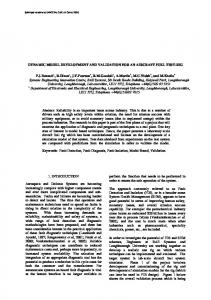
that the GLODAP product is compiled from a number of cruise observations, which are mainly derived from the World Ocean Circulation Experiment (WOCE), Joint Global Ocean Flux Study (JGOFS), and Ocean Atmosphere Carbon Exchange Program (OACES) carried out during the 1990s (see Key et al. 2004 for the time periods of these cruises). In addition, several other historical cruise observations from the 1970s and 1980s are also included in the GLODAP data. The sampling population consists of 9618 global observation stations (from 95 cruises) during the period 1985–99, and 2393 global observation stations during the period 1972–90 (21 cruises). There are very few observation stations that were used from historical cruises that date back to 1972. In GLODAP, all these observations are combined into one dataset, and thus they do not exactly represent the scenario of a particular year. However, the majority of samples used in the GLODAP dataset is collected between the period 1990 and 1999 during WOCE cruises, which consist of 80% of the total sampling from 78% of the total cruises. Thus, it is possible to represent the data as a scenario of 1993 or 1995. In this study, we compare the model year 1995 with the observations, unless otherwise specified. This is true especially in the Atlantic Ocean, where the majority of observations included in GLODAP are carried out during the early 1990s. Before proceeding into real-time runs, we optimize a suitable model configuration from a number of test experiments carried out with different choices of vertical mixing configurations. The results of these test experiments are then compared with CFC-11 observations and an optimum configuration is found. In these test experiments, the main focus is given to tuning the vertical mixing. Such test experiments to find a best configuration is necessary because the offline transport models are operating on some parent model outputs with variable periodicities of input data. In this case, the performance of transport models is sensitive to the frequency of input data, and so the model behaves slightly different for different sets of input feeding. Thus, before getting into application runs, the model performance must be tested with different sets of configurations and a best case should be found. A number of test experiments are conducted, among which a suite of six are mentioned here. In these runs,
the variable parameters are either one or a combination of (i) mixed layer depth, (ii) monthly climatology of wind stress or a globally constant wind stress for KPP, and (iii) inclusion or exclusion of subgrid-scale parameterizations. The mixed layer depth of the GFDL product that we used in this study is somewhat “weaker” than the observations of Kara et al. (2000). Thus, the MLD is multiplied by a factor of 1, 1.5, and 2 for individual test runs. These three cases are then combined with or without GM subgrid-scale parameterizations and with monthly wind stress climatology or a constant wind stress of 0.03 N m⫺2. Table 1 summarizes the experiment cases. Note that all these sensitivity experiments have the same CFC-11 forcing as in OCMIP-2. Figure 1 shows the CFC-11 simulations of six runs and compares them with the corresponding observations. The plots represent the zonal integral of Atlantic CFC-11 column inventories during 1995. The units are picomole meters squared per kilogram. It is evident that the model’s performance varies considerably among different combinations of configurations. A large difference in the model performance is obvious in the Southern Hemisphere deep convection regions (between 60° and 40°S). The best match with the observation is obtained by the run 2_MLD_GM_Clim (2 times the MLD adopted from GFDL product, with GM parameterization and a climatological stress). The prediction statistical skill and error estimates for each of these test runs are shown in Table 2; the correlation between observations and each of these test runs gives us a quantitative evaluation of the cases presented here. The discrepancy in the Southern Hemisphere among the different model configurations is mainly due to the difference in the vertical mixing. It is obvious from the figure that the mapping of the same MLD as that of the input data underestimates the vertical mixing in the Southern Hemisphere. However, a constant wind stress of 0.03 N m⫺2 erodes the mixing further and deeper, although this is not satisfactory in the Northern Hemisphere. A choice of 1.5 times the MLD gives s better simulation in the Northern Hemisphere, while that in the Southern Hemisphere is still weaker. Column inventories along 20° and 30°W in the Atlantic are shown separately in the bottom panels. It is obvious that the vertical mixing is sensitive to the choice of MLD. The standard deviation of CFC-11 from the mean
15 JUNE 2008
2759
VALSALA ET AL.
FIG. 1. CFC-11 concentration integrated zonally and vertically over (top) the Atlantic Ocean and inventories along (bottom left) 30°W and (bottom right) 20°W. Units are (top) pmol m2 kg⫺1 and (bottom) pmol m kg⫺1.
inventories in the Atlantic Ocean is 0.69 pmol m2 kg⫺1 (Fig. 1, top; Table 2). Although the standard deviation of three test simulations are close to this value, a high correlation coefficient of 0.95 leads us to prefer the case 2_MLD_GM_Clim as being more suitable (Table 2). For this particular case, the statistical skill score (as suggested in Taylor 2001) has a maximum value of
0.95, and a centered pattern of the root-mean-square (RMS) difference has a minimum value of 0.23. Thus, we opt for a choice of 2 times MLD with climatological surface wind stress forcing as the best case, and we consider only this case for the rest of our experiments. We note, however, that this configuration does not imply the ultimate choice for this model; in-
TABLE 2. Statistical summary of test-run simulations shown in Fig. 1. Acronyms are same as those given in Table 1. Data std dev ⫽ 0.69 Correlation Std dev Skill RMS
1_MLD_GM_Clim 1_MLD_GM_0.03 2_MLD_GM_Clim 2_MLD_GM_0.03 1.5_MLD_GM_Clim 1.5_MLD_GM_0.03 0.88 0.39 0.69 0.39
0.87 0.46 0.80 0.37
0.94 0.60 0.95 0.23
0.91 0.64 0.94 0.28
0.92 0.62 0.94 0.28
0.89 0.56 0.87 0.32
2760
JOURNAL OF CLIMATE
stead, it only means that it is the best-suited configuration for the input data used in this study.
a. Comparison with observations The deepest penetration of CFC-11 in the global ocean is found in the North Atlantic, where the deepwater formation sites are located. Thus, the deep-water formation process should be simulated well in the model to capture this deep penetration of CFC-11. Therefore, we concentrate our discussion more on the model’s Atlantic Ocean transports and its comparison with observations. Figure 2 shows the column inventory of CFC-11 (vertically integrated) during 1995 obtained from our model and the corresponding observations obtained from GLODAP. The units are picomole meters per kilogram. Although the column inventories do not represent the deep penetration of tracers explicitly, we begin our comparison for a large-scale model simulation and then proceed to a more detailed comparison of regional vertical profiles. A remarkable similarity in the column inventories of CFC-11 is noticeable in the Atlantic. The deepest convection in the North Atlantic is located in the Labrador Sea, where the mixed layer extends as deep as 800–1300 m (Canuto et al. 2004). Observations show that maximum CFC-11 column inventories are located in the Labrador Sea. The model captures this maximum appreciably well with a magnitude of 11 ⫻ 103 pmol m kg⫺1 as in the observations. A second maximum inventory is located north of 70°N in the Greenland and Norwegian Seas. However, there is no available observation of CFC-11 to validate these sites. The meridional gradient of the CFC-11 column inventory in the model is remarkably similar to that of observations. The North Atlantic water mass is subducted at various locations, such as the Labrador Sea, Denmark Strait, and Iceland–Scotland Overflow regions. CFC-11 in these deep regions is advected southward mainly along with the deep western boundary currents. This southward advection along the western boundary is visible by coastally elongated contours in the observations. It is appreciably represented in the model with a good agreement in magnitude compared to the observations. Further, this southward component of CFC-11 is advected eastward in the deep ocean, which makes a meridional gradient of CFC-11. It is noted that the model has a steeper north–south gradient of CFC-11 than those in the observations. In the Southern Hemisphere, the high CFC-11 inventory is located between 40° and 50°S. This is the region where deep convection in the Southern Hemisphere is observed. The maximum penetration of CFC-11 in this belt is found near the South American continent. This
VOLUME 21
deeply convected water is advected horizontally to the east at a depth of 1000 m and marks a high-concentration belt between 40° and 50°S. This region demarcates the boundary of the subtropical gyre with the polar front, and the water mass is ventilated from the depth below the mixed layer to the deep ocean. This water is referred to as the South Atlantic Mode Water (SAMW), which is a key portion in the southern Atlantic where oceanic uptake of CO2 is prominent (Dutay et al. 2002). In the Antarctic Ocean, the model shows a mismatch with the observation at 40°W. This may be due to a limitation in the ice-water formation in the model circulations. The large-scale transport of the model is in good agreement with the observations. This is further evaluated by estimating the error in the model column inventory, which is due to either one or a combination of uncertainties in large-scale circulations and diagnostics used in the model. The error estimates are shown in Fig. 2 (bottom). Here, the error represents the model drift from the observations. It can be seen that the predictions fall within an overall error bar of ⫾0.4 ⫻ 103 pmol m kg⫺1 in the Atlantic. This is within a range of ⫾10% of the observations. However, the meridional error difference is as large as the maximum error of 1.5 ⫻ 103 pmol m kg⫺1. In the subtropics, at midlatitude and high latitude, the error bar is within ⫾10%, while in the equatorial region, the error is projected as high as 30%. Simulating an accurate meridional transport of tracers is a real challenge in transport models. For example, the atmospheric transport model has large error bars in the interhemispheric gradient. Given the values of 9 ⫻ 103 pmol m kg⫺1 meridional difference of CFC11 observed in the North Atlantic, an error gradient of 1.5 ⫻ 103 pmol m kg⫺1 reasons an error of 16% in the simulated meridional gradient of CFC-11. The modelcentered RMS difference of CFC-11 uptake in the entire Atlantic is 0.23 pmol m2 kg⫺1, which is ⫾5% of the observed mean (Fig. 1; Table 2). The detailed examination of the vertical profile of the model CFC-11 will further explain this error behavior in the model. Although the column inventory of CFC-11 in the Atlantic Ocean is well simulated in the model, a detailed vertical structure should be assessed with the observations because the inventories do not provide exact information about the vertical profile. To assess the model’s ability to simulate deep convection and ventilation, we compare a few vertical sections in the Atlantic Ocean with the observations. Figure 3 shows the North Atlantic cross section along 30°W. The examination of the North Atlantic sections provides the ventilation pathways of the CFC. The key water masses forming in
FIG. 2. Column inventory of CFC-11 from (left) observations and (middle) model during 1995. The model error is shown as the difference from the (right) observations. Units are 103 pmol m kg⫺1.
15 JUNE 2008 VALSALA ET AL.
2761
2762
JOURNAL OF CLIMATE
VOLUME 21
FIG. 3. Model-simulated CFC-11 in the North Atlantic (middle) along 30°W during 1995, (left) corresponding observations, and (right) model error. Units are pmol kg⫺1.
the North Atlantic consist of North Atlantic Deep Water (NADW), which is composed of Lower North Atlantic Deep Water (LNADW) and Upper North Atlantic Deep Water (UNADW). The elevated contours below 1000 m in the deep ocean are due to the renewal of NADW. This is reproduced reasonably well in the model. The elevated contours in the observations show a deep-core maximum between 1500 and 2000 m, which is the UNADW subducted from the base of the mixed layer. The subducted water is shown to be carried farther eastward by the deep ocean currents at this depth. In the model, this core is found above 1500 m. This is partially due to the relatively limited supply of UNADW eastward, which is subducted at the western
coast. It is noted that the contour of 0.5 in the model stretches to a depth of 3000 m, as in the observations. We can assess in more detail the NADW ventilation characteristics from the zonal section at 24°N (Fig. 4), as shown in Dutay et al. (2002). The classical 24°N section shows an obvious double core of high concentration at the western boundary, each located between 3000 and 4000 m and between 1500 and 1800 m. The former is the LNADW, which is supplied from the Denmark Strait Overflow Water (DSOW) and Iceland–Scotland Overflow Water (ISOW), which is then carried south along with the deep western boundary currents. However, there is no obvious deep core reproduced in the model. It should be noted that a high-
FIG. 4. Model-simulated CFC-11 in the North Atlantic (middle) along ⬃24°N during 1995, (left) corresponding observations, and (right) model error. Units are pmol kg⫺1.
15 JUNE 2008
VALSALA ET AL.
2763
FIG. 5. Model-simulated CFC-11 in the North Atlantic (middle) along 40°W during 1995, (left) corresponding observations, and (right) model error. Units are pmol kg⫺1.
resolution version of the offline model by Gupta and England (2004) also didn’t resolve this double-core structure. Moreover, none of the OCMIP-2 models (most of them are online models) reproduced this double-core structure of CFC. Thus, a comparison between the previous results of OCMIP-2, Gupta and England (2004), and our results shows that the resolution is not the reason for the absence of such a double-core system. Also, our results show that the shallow core (between 1500 and 1800 m) elongates further down to 3000 m. One possibility for the absence of an obvious double-core system in the models may be because of the increased diapycnal mixing that occurs at the region with an intense western boundary current, which smears the cores and mixes each other (although a deep western boundary current exists as distinct cores). It is also noteworthy that the only candidate in OCMIP-2 to resolve this feature reasonably well is Germany’s Alfred Wegener Institute for Polar and Marine Research (AWI) model, which was originally an adjoint model that derived circulation from hydrographic and geochemical data (Dutay et al. 2002). Another section along the North Atlantic we have examined is the 40°W section (Fig. 5), which passes through the “mouth” of the Labrador Sea where it opens to the Atlantic. This is the location where deep penetration of CFC-11 is noted in both the observation and the model. The section shows a reasonable similarity between the observation and the model. The deepest penetration is 4000 m for the contour of 0.5 pmol kg⫺1 in both the observation and the model. The tonguelike shape in the model near 55°N shows the mode water formation and subduction at the base of
the mixed layer. This is in close agreement with the observation. A meridional section from the South Atlantic is shown in Fig. 6. The location of the section is 0°W, which is close to the AJAX section as shown in Dutay et al. (2002). The SAMW formation is reasonable in the model with a maximum penetration depth of nearly 1500 m. This is in good agreement with the observations. The maximum near the southern boundary is somewhat overestimated in the model and elongated deeper. The observation data in GLODAP didn’t show enough concentration in the deep southern boundary as seen from the AJAX section, and the model didn’t show any high concentration deep in the southern boundary. In all the cross sections we presented here, an enhanced vertical mixing in the equatorial region is found in the model, especially at the section close to the American continent (or western part of the Atlantic Ocean). This is not obvious in the observations. The modeled equatorial mixing is relatively stronger than in reality, especially in the western boundary. This is equally reflected in the equatorial region column inventory and resulted in a large error there (Fig. 2, bottom). However, the relative concentration below the observed limit in the equatorial region is smaller and will not contribute much to the total CFC-11 uptake in the models.
b. Comparison with OCMIP-2 participant models In this section, we compare our results with models that participated in OCMIP-2. This comparison will help us to demonstrate the advantages of using high-
2764
JOURNAL OF CLIMATE
VOLUME 21
FIG. 6. Model-simulated CFC-11 in the South Atlantic (middle) along ⬃0° during 1995, (left) corresponding observations, and (right) model error. Units are pmol kg⫺1.
resolution offline models to improve the accuracy in transport calculations. This comparison is possible even though the models of OCMIP-2 have a wide range of resolution and vary in their behavior according to the physics included in each model. Any appreciable differences we see among these models and our offline solutions may be attributable to a number of reasons related to the difference in the circulation field resolved in each of these models. The ideal way to compare our result with an OCMIP-2 candidate would be to begin with a comparison of physical fields (i.e., circulation and mixing details) and then move to CFC-11. However, obtaining such fields and a detailed comparison with assimilated circulation that we used in our simulation is impractical and out of our topic. At the same time, a comparison of our offline solutions with CFC-11 observations has shown good agreement, which in turn shows that a comparison of our model results with candidate models of OCMIP-2 will provide a performance assessment in CFC-11 simulation without having a oneto-one detailed comparison of the circulation field between OCMIP-2 candidates and the offline input that we used in our simulation. Moreover, we have used the same surface forcing for CFC-11 as that of OCMIP-2 experiments, which enables us to make a direct comparison. We chose eight models from OCMIP-2 participants for the comparison here. This selection is based on referring to Dutay et al. (2002). Only those candidates that show a reasonable agreement with the observations are included here: Commonwealth Scientific and Industrial Research Organisation (CSIRO), Institute for Global Change Research, Tokyo, Japan (IGCR), L’Institut Pierre-Simon Laplace Coupled Model
(IPSL), Lawrence Livermore National Laboratory (LLNL), Massachusetts Institute of Technology (MIT), National Energy Research Scientific Computing Center (NERSC), Princeton University experiment-2 (PRINCE2), and Southampton Oceanography Centre (SOC; see Dutay et al. 2002). All of these models had been run based on the OCMIP-2 CFC-11 flux protocol from 1938 to 1997. We will present a quantitative comparison between our model and these models in the Atlantic. Figure 7 shows the zonally integrated CFC-11 column inventories in the entire Atlantic (100°W ⬃20°E), as simulated by the candidate models of OCMIP-2, our model, and the corresponding observations. This provides a quantitative comparison of CFC-11 simulated by each of these models. The northern Atlantic ventilation process is captured by participating models of OCMIP-2, although the majority underestimates it. A close examination indicates that our model has excellent agreement with the observations in the subduction zone of the northern Atlantic. The model spread is relatively larger in the northern Atlantic than in the Southern Ocean. Among the OCMIP-2 candidates, a double peak in the North Atlantic is captured only in MIT, IGCR, and NERSC, although the amplitude is almost double in NERSC. The other candidates do not have an obvious double peak. It is noticeable that our model captures these two maxima remarkably well compared to the observations. In the Southern Ocean, all models have reasonable performance. Also in this case, our model reproduces both the phase and amplitude of the observed CFC-11 inventory appreciably well. A minimum in CFC-11 inventories around 51°S and a secondary maximum
15 JUNE 2008
VALSALA ET AL.
2765
FIG. 7. Zonally integrated column inventories of CFC-11 in the entire Atlantic from the candidate models of OCMIP-2, our model, and corresponding observations. Units are pmol m2 kg⫺1.
around 57°S are well captured only in our model and LLNL. All other models have a wide range of CFC-11 inventory in the Southern Hemisphere. The deviation of NERSC from the mean state is too large, and the IGCR model also overestimates CFC-11 inventory in the Southern Ocean. None of the models (including ours) maintains a shallow penetration of CFC-11 that is bound to 70°S, except LLNL. This may be due to the inconsistent ice parameterizations included in the models. The NERSC model shows extremely localized high concentrations in the subduction zone of the SAMW region. In the equatorial region, our model overestimates vertical mixing as compared to the observations as well as the other candidate models of OCMIP-2. However, it is noteworthy that the equatorial pattern is captured by our model even though the mixing is exaggerated. The other candidate models of OCMIP-2 underestimate the vertical mixing in the equatorial region, except MIT, which shows an appreciable match of phase and amplitude with the observations. The comparison with the other models of OCMIP-2 shows that our model’s performance falls within the range achieved by the candidate models of OCMIP-2. These models have varying levels of agreement and disagreement with the observation at various parts of the ocean. For example, IGCR and MIT perform reasonably well in the North Atlantic but have a poor performance in the South Atlantic. LLNL exhibits excellent performance in the South Atlantic but is biased
toward underestimation in the northern Atlantic. Some candidates exaggerate the amplitude, while others have different phases. Our model has a good agreement in both amplitude and phase at the northern as well as the Southern Ocean, while it is exaggerated in amplitude in the equatorial region. By this way of comparison, it is difficult to conclude which model can most accurately simulate the observations. To achieve a more quantitative comparison among these models as well as with the observations and also to find the skill of these models to simulate a scenario close to reality, we opt for a representation of model statistics as provided in Taylor (2001). Figure 8 shows the standard deviations and correlations (with the observations) of the plots given in Fig. 7. The radial distance from the origin is proportional to the standard deviation and the cosine of the angle between the radial line, and the abscissa is the correlation between each model and the observations. To compare the model’s performance in this way, we need a reference point that represents the standard deviation of observations (as seen in Fig. 8) and a correlation coefficient of 1. Any point in the map is thus defined by a combination of standard deviation and correlation. The models with the best performance in simulating both amplitude and phase of observations will thus lie close to the reference point. A statistical skill score based on standard deviation and correlation of each model is found as that given in Taylor (2001), with a maximum expectation correlation coefficient of R0 ⫽ 0.99.
2766
JOURNAL OF CLIMATE
VOLUME 21
FIG. 8. Model std dev and correlation with reference data (GLODAP) are displayed as in Taylor (2001). The radial lines are labeled by the cosine of the angle made with the abscissa. The reference data have a std dev of 0.74. Our model has a std dev of 0.60 and a correlation coefficient of 0.95. Skill values are given in brackets.
The observation has a standard deviation of 0.74 pmol m2 kg⫺1. The OCMIP-2 candidate models spread in a standard deviation band of 0.60 to 1.62, a correlation band of 0.89 to 0.67, and a skill band of 0.92 to 0.48. Our model has a standard deviation of 0.60 and a skill value of 0.94, which is the highest skill score compared to other models shown here. However, some of the OCMIP-2 models have a standard deviation that is closer to the observations than that of our model. For example PRINCE2, SOC, and National Center for Atmospheric Research (NCAR) models have better standard deviations, but their correlations are low compared to our model. This shows that these models simulated a more accurate amplitude of the north–south column inventory, but the phase mismatches. On the other hand, in our model, the good correlation and relatively weaker standard deviation (compared to PRINCE2, SOC, and NCAR) mean that the phase of the north–south Atlantic CFC-11 inventory is good, but the amplitude is affected. From Fig. 7, it is obvious that the equatorial exaggeration of vertical mixing is the reason for this amplitude mismatch in our model. How-
ever, the skill measure (which is a collective measure of standard deviation and correlation) shows that our model outperforms the OCMIP-2 candidate models in the Atlantic with a skill score of 0.94, which is the highest among the models compared here.
c. Error comparison with OCMIP-2 participant models The Taylor (2001) diagram explicitly shows the correlation coefficient between the observed field and the model as well as their centered RMS differences, along with the ratio of the standard deviations of the two patterns. The centered RMS difference between the model and the observations is proportional to their distance apart in the same units as the standard deviation. This distance is 0.14 ⫻ 1010 pmol m2 kg⫺1 in our model. This represents the RMS difference of the model north–south column inventory from the observations. In our model, this corresponds to an error of ⫾8% from the observed mean of north–south CFC-11 column inventory. Among the OCMIP-2 participant models, CSIRO and LLNL have the same RMSE difference as
15 JUNE 2008
VALSALA ET AL.
ours. The RMSE differences of NCAR and MIT are ⫾4% and ⫾9%, respectively, which shows that these models (including ours) have error in the amplitude of the north–south column inventory. In our model, this is due to the exaggeration of vertical mixing and the CFC11 uptake in the equatorial region. The overall error in the tropics in our model is 30%. However, the observations suggest that the tropical Atlantic contains only 18.7% of the total CFC-11 of the entire Atlantic, and thus a model error of 30% in the tropics means only an error of 6% in the total CFC-11 uptake. The minimum RMSE difference of OCMIP-2 participants is found in PRINCE2 and SOC, which have an error of ⫾4% from the mean north–south column inventory.
5. Discussion and conclusions It is evident from Figs. 7, 8 that our model captures the majority of the column inventory features of CFC11 remarkably well and has a high skill score compared to the OCMIP-2 participants. Thus, it is useful to point out the reasons for this improved performance in our model compared to that of other candidates of OCMIP2. The main reason may be the higher resolution of our model compared to the very coarse resolutions used in OCMIP-2. Thus, it is evident that the restriction of resolution because of the cost of computational time in the online models has affected the accuracy in transport, which can be effectively solved by adapting an offline version with reasonable ocean circulation—a real advantage of offline models. This conclusion is consistent with the model results of Gupta and England (2004). Another reason for improvement in our model may be the assimilated oceanic currents that we used to find the transport. Apart from the resolution, the limitations in the model physics also affect the performance of online simulations. Thus, by having an assimilated current as prior information with appreciable periodicity to represent the dominant mode of variability (monthly or weekly), there is a good chance to achieve high accuracy in transport calculations using offline models. Our model results show that even though the vertical mixing and horizontal subgrid-scale processes are parameterized in the offline model, the accuracy present in advective components inherited from the assimilated field plays a potential role in improving the transport calculation. Together with the assimilated advection— if it is possible to provide other mixing coefficients from the parent model itself—the offline model could be tuned to get a further and more accurate transport. The accuracy of transport has a critical role in modeling the oceanic uptake of carbonaceous tracers. For instance,
2767
the equilibration time scale (time scale to reach an equilibrium between the partial pressures at the ocean– air interface) of CFC-11 is relatively short. Thus, vertical or horizontal transport of surface CFC-11 to any long distances before it equilibrates locally has potential influence on the equilibration time scale of air–sea fluxes and hence the total uptake by the oceans. Because the ocean acts as a large-scale sink for carbonaceous tracers in the atmosphere, like anthropogenic CO2, it is vital to quantify the role of oceans on the life cycle of CO2 in the hydrosphere and atmosphere. Inadequate observations of parameters that are necessary for the estimation of air–sea exchange of CO2 and other carbonaceous tracers always force us to depend largely on climate models to assess the fate of these trace materials. However, the climate models that do this job have to undergo several compromises on computational resources and poorly understood carbon physics, mostly resulting in unsatisfactory estimates of carbon fluxes. Thus, the roles of accurate transport calculation have a significant impact on quantifying the oceanic sources and sinks of carbonaceous substances. For the oceans, our study puts forward a suggestion to depend on assimilated ocean currents and other parameters that are mostly close to reality to estimate the transport of trace materials with a cost-effective computation. Fletcher et al. (2006a,b) and Gloor et al. (2003) have used inverse methods to find the oceanic sources and sinks of anthropogenic as well as natural CO2. The accuracy of the inversion depends solely on the accuracy of transport functions. The comparison of several OCMIP-2 candidate models of coarse resolution [some of these models are also used in inversion experiments of Fletcher et al. (2006a,b)] showed notable differences in performance as is described in their paper. Comparing our model’s results with these models, as well as with the observations, shows that our model has a relatively higher skill score. Therefore, our model is a potential candidate for the inversion studies as used in Fletcher et al. (2006a,b). We attribute the reasons for this accuracy in our model to the high resolution and to the assimilated ocean currents and hydrography that we used, which are still compatible with cost-effective computation. Certain shortcomings are present in the current configuration of our model, especially in the equatorial mixing. The mixed layer depth criteria in our bestsuited configuration for the set of input data resulted in a stronger vertical mixing in the equatorial region, especially at the western boundary. We have investigated the reason for this behavior in the model in connection with its 2 times the MLD mapping in the present con-
2768
JOURNAL OF CLIMATE
figuration. However, Fig. 1 shows that even with a scaling factor of 1, the equatorial mixing is exaggerated. The high shear present in the equatorial current may be the reason for the increased mixing resolved in KPP. The numerical diffusion, which is larger in faster current regions, can also be testament to this exaggerated mixing (Kantha and Clayson 2000). Another drawback of the present simulation is that we limited our input data to a monthly periodicity mainly because of unavailability of high-frequency data. Choosing a high-frequency input data such as daily periodicity, if available, could improve the model’s performance. The growing availability of reanalysis products for ocean circulation gives us hope to use this model with high-frequency input data in the future. In addition, a comparison of simulations of this model using different assimilated ocean products will give us a clue to the potential biases in the model, such as exaggerated equatorial mixing. A similar intercomparison of transport derived using different assimilated ocean currents is indeed under way. Moreover, our future task is to use this model for coupled ocean–atmosphere inversions for CO2 fluxes and with OCMIP-2-type biogeochemical modeling experiments by coupling with an ecosystem model.
6. Summary An offline passive tracer transport model is designed and discussed here. This model was developed at the National Institute for Environmental Studies (NIES) under the carbon cycle research project inside the GOSAT modeling group. The model equations for tracer evolution, vertical mixing, horizontal diffusion, and other subgrid-scale parameterizations are detailed. The model borrows offline fields from precalculated monthly archives of assimilated ocean currents, temperature, and salinity, and evolves a prognostic passive tracer with a prescribed surface forcing. The model’s performance is validated by simulating the CFC-11 cycle in the ocean starting from the preindustrial period (1938) with observed anthropogenic perturbations of atmospheric CFC-11 to comply with the OCMIP-2 flux protocol. The model results are compared with ship observations as well as with the results of the candidate models of OCMIP-2 and a performance is assessed. The model simulates the deep ventilation processes in the Atlantic Ocean appreciably well and yields a good agreement in the column inventory of CFC-11 compared to the observation. The error estimates show that the models intake of CFC-11 is within an overall error bar of ⫾8% in the Atlantic, while an exaggeration in tropical CFC-11 intake is noted. The spatial pattern of
VOLUME 21
CFC-11 intake is well simulated in the model, with an overall Atlantic correlation of 0.95 compared to the observations. The statistical skill comparison test with the OCMIP-2 participant models shows that our model performs appreciably well in the CFC-11 column inventory simulation. The spatial pattern of CFC-11 inventories in our model has a higher correlation with the observations than the OCMIP-2 participant models. The improvements in performance of our model compared to other models are attributed to its higher resolution and assimilated offline inputs feeding. This shows a potential role in improving transport calculation in the ocean with cost-effective computation. Acknowledgments. We are thankful for the financial support from GOSAT operating at NIES for the development of this model. The computational resource is provided by the supercomputer facility at NIES. The offline fields are provided by GFLD in Princeton, New Jersey. Comments and suggestions from various modeling groups inside and outside of Japan have helped to pinpoint and troubleshoot our model’s physics and code. The comments from one anonymous reviewer have helped us to refer to a very relevant paper, which had skipped from our attention. The model code will be provided for research purposes upon request. REFERENCES Asselin, R., 1972: Frequency filter for time integrations. Mon. Wea. Rev., 100, 487–490. Bryan, K., and L. J. Lewis, 1979: A water mass model of the world ocean. J. Geophys. Res., 84, 2503–2517. Canuto, V. M., A. Howard, P. Hogan, Y. Cheng, M. S. Dubovikov, and L. M. Montenegro, 2004: Modeling ocean deep convection. Ocean Modell., 7, 75–95. Dutay, J.-C., and Coauthors, 2002: Evaluation of ocean model ventilation with CFC-11: Comparison of 13 global ocean models. Ocean Modell., 4, 89–120. Enting, I. G., 2002: Inverse Problems in Atmospheric Constituent Transport. Cambridge University Press, 392 pp. Fletcher, S. E. M., and Coauthors, 2006a: Inverse estimates of anthropogenic CO2 uptake, transport, and storage by the ocean. J. Geophys. Res., 20, GB2002, doi:10.1029/ 2005GB002530. ——, and Coauthors, 2006b: Inverse estimates of the oceanic sources and sinks of natural CO2 and the implied oceanic carbon transport. J. Geophys. Res., 21, GB1010, doi:10.1029/ 2006GB002751. Fukumori, I., T. Lee, B. Cheng, and D. Menemenlis, 2004: The origin, pathway, and destination of Niño-3 water estimated by a simulated passive tracer and its adjoint. J. Phys. Oceanogr., 34, 582–604. Gent, P. R., and J. C. McWilliams, 1990: Isopycnal mixing in ocean circulation models. J. Phys. Oceanogr., 20, 150–155. Gloor, M., N. Gruber, J. Sarmiento, C. L. Sabine, R. A. Feely, and C. Rödenbeck, 2003: A first estimate of present and preindustrial air–sea CO2 flux patterns based on ocean interior
15 JUNE 2008
VALSALA ET AL.
carbon measurements and models. Geophys. Res. Lett., 30, 1010, doi:10.1029/2002GL015594. Gupta, A. S., and M. England, 2004: Evaluation of interior circulation in a high-resolution global ocean model. Part I: Deep and bottom waters. J. Phys. Oceanogr., 34, 2592–2614. Hecht, M. W., W. R. Holland, and P. J. Rasch, 1995: Upwindweighted advection schemes for ocean tracer transport: An evaluation in a passive tracer context. J. Geophys. Res., 100, 20 763–20 778. Hellerman, S., and M. J. Rosenstein, 1983: Normal monthly wind stress over the world ocean with error estimates. J. Phys. Oceanogr., 13, 1093–1104. Hourdin, F., and O. Talagrand, 2002: Eulerian backtracking of atmospheric tracers. I: Adjoint derivation and parametrization of subgrid-scale transport. Quart. J. Roy. Meteor. Soc., 132, 567–583. ——, ——, and A. Idelkadi, 2002: Eulerian backtracking of atmospheric tracers. II: Numerical aspects. Quart. J. Roy. Meteor. Soc., 132, 585–603. Josey, S. A., E. C. Kent, and P. K. Taylor, 1999: New insights into the ocean heat budget closure problem from analysis of the SOC air–sea flux climatology. J. Climate, 12, 2856–2880. Kantha, L. H., and C. A. Clayson, 2000: Numerical Models of Oceans and Oceanic Processes. International Geophysics Series, Vol. 66, Academic Press, 940 pp. Kara, A. B., P. A. Rochford, and H. E. Hulburt, 2000: An optimal definition for ocean mixed layer. J. Geophys. Res., 105, 16 803–16 821. Key, R. M., and Coauthors, 2004: A global ocean carbon climatology: Results from Global Ocean Data Analysis Project
2769
(GLODAP). J. Geophys. Res., 18, GB4031, doi:10.1029/ 2004GB002247. Khatiwala, S., 2007: A computational framework for simulation of biogeochemical tracers in the ocean. Global Biogeochem. Cycles, 21, GB3001, doi:10.1029/2007GB002923. ——, M. Visbeck, and M. A. Cane, 2005: Accelerated simulation of passive tracers in ocean circulation models. Ocean Modell., 9, 51–69. Large, W. G., J. C. McWilliams, and S. C. Doney, 1994: Oceanic vertical mixing: A review and a model with a nonlocal boundary layer parameterization. Rev. Geophys., 32, 363–403. McKinley, G. A., M. J. Follows, and J. Marshall, 2004: Mechanism of air–sea CO2 flux variability in the equatorial Pacific and North Atlantic. Global Biogeochem. Cycles, 18, GB2011, doi:10.1029/2003GB002179. Mellor, G. L., and T. Yamada, 1982: Development of a turbulence closure model for geophysical fluid problems. Rev. Geophys., 20, 851–875. Pacanowski, R. C., and S. M. Griffies, 1999: The MOM3 manual. Geophysical Fluid Dynamics Laboratory Ocean Group Tech. Rep. 4, 680 pp. Redi, M., 1982: Oceanic isopycnal mixing by coordinate rotation. J. Phys. Oceanogr., 12, 1154–1158. Taylor, K. E., 2001: Summarizing multiple aspects of model performance in a single diagram. J. Geophys. Res., 106, 7183– 7192. Valsala, K. V., and M. Ikeda, 2007: Pathways and effects of the Indonesian Throughflow water in the Indian Ocean using particle trajectory and tracers in an OGCM. J. Climate, 20, 2994–3017.