Design Challenges and Misconceptions in Neural

Design Challenges and Misconceptions in Neural Sequence Labeling Jie Yang, Shuailong Liang, Yue Zhang Singapore University of Technology and Design {jie yang, shuailong liang}@mymail.sutd.edu.sg yue [email protected]

Abstract We investigate the design challenges of constructing effective and efficient neural sequence labeling systems, by reproducing twelve neural sequence labeling models, which include most of the state-of-the-art structures, and conduct a systematic model comparison on three benchmarks (i.e. NER, Chunking, and POS tagging). Misconceptions and inconsistent conclusions in existing literature are examined and clarified under statistical experiments. In the comparison and analysis process, we reach several practical conclusions which can be useful to practitioners.

1

Introduction

Sequence labeling models have been used for fundamental NLP tasks such as POS tagging, chunking and named entity recognition (NER). Traditional work uses statistical approaches such as Hidden Markov Models (HMM) and Conditional Random Fields (CRF) (Ratinov and Roth, 2009; Passos et al., 2014; Luo et al., 2015) with handcrafted features and task-specific resources. With advances in deep learning, neural models have given state-of-the-art results on many sequence labeling tasks (Ling et al., 2015; Lample et al., 2016; Ma and Hovy, 2016). Words and characters are encoded in distributed representations (Mikolov et al., 2013) and sentence-level features are learned automatically during end-to-end training. Many existing state-of-the-art neural sequence labeling models utilize word-level Long Short-Term Memory (LSTM) structures to represent global sequence information and a CRF layer to capture dependencies between neighboring labels (Huang et al., 2015; Lample et al., 2016; Ma and Hovy, 2016; Peters et al., 2017). As an alternative, Convolution Neural Network (CNN) (LeCun et al., 1989) has also been used for its ability of parallel computing, leading to an efficient training and decoding process. Despite them being dominant in the research literature, reproducing published results for neural models can be challenging, even if the codes are available open source. For example, Reimers and Gurevych (2017b) conduct a large number of experiments using the code of Ma and Hovy (2016), but cannot obtain comparable results as reported in the paper. Liu et al. (2018) report lower average F-scores on NER when reproducing the structure of Lample et al. (2016), and on POS tagging when reproducing Ma and Hovy (2016). Most literature compares results with others by citing the scores directly (Huang et al., 2015; Lample et al., 2016) without re-implementing them under the same setting, resulting in less persuasiveness on the advantage of their models. In addition, conclusions from different reports can be contradictory. For example, most work observes that stochastic gradient descent (SGD) gives best performance on NER task (Chiu and Nichols, 2016; Lample et al., 2016; Ma and Hovy, 2016), while Reimers and Gurevych (2017b) report that SGD is the worst optimizer on the same datasets. The comparison between different deep neural models is challenging due to sensitivity on experimental settings. We list six inconsistent configurations in literature, which lead to difficulties for fair comparison. • Dataset. Most work reports sequence labeling results on both CoNLL 2003 English NER (Tjong Kim Sang and De Meulder, 2003) and PTB POS (Marcus et al., 1993) datasets (Collobert et al., 2011; Huang et al., 2015; Ma and Hovy, 2016). Ling et al. (2015) give results only on POS dataset, while some This work is licenced under a Creative Commons Attribution 4.0 International Licence. //creativecommons.org/licenses/by/4.0/

Licence details: http:

Models No Char

Char LSTM

Char CNN

Word LSTM+CRF Huang et al. (2015)* Lample et al. (2016) Strubell et al. (2017)* Lample et al. (2016) Rei (2017) Liu et al. (2018) Ma and Hovy (2016) Chiu and Nichols (2016)* Peters et al. (2017)

Word LSTM Ma and Hovy (2016) Strubell et al. (2017)*

Word CNN Strubell et al. (2017)*

Lample et al. (2016)

Word CNN+CRF Collobert et al. (2011)* dos Santos et al. (2015) Strubell et al. (2017)* No existing work

Ma and Hovy (2016)

dos Santos et al. (2015)

Santos and Zadrozny (2014)

No existing work

Table 1: Neural sequence labeling models in literatures. * represents using handcrafted neural features. papers (Chiu and Nichols, 2016; Lample et al., 2016; Strubell et al., 2017) report results on the NER dataset only. dos Santos et al. (2015) conducts experiments on NER for Portuguese and Spanish. Most work uses the development set to select hyperparameters (Lample et al., 2016; Ma and Hovy, 2016), while others add development set into training set (Chiu and Nichols, 2016; Peters et al., 2017). Reimers and Gurevych (2017b) use a smaller dataset (13862 vs 14987 sentences). Different from Ma and Hovy (2016) and Liu et al. (2018), Huang et al. (2015) choose a different data split on the POS dataset. Liu et al. (2018) and Hashimoto et al. (2017) use different development sets for chunking. • Preprocessing. A typical data preprocessing step is to normize digit characters (Chiu and Nichols, 2016; Lample et al., 2016; Yang et al., 2016; Strubell et al., 2017). Reimers and Gurevych (2017b) use fine-grained representations for less frequent words. Ma and Hovy (2016) do not use preprocessing. • Features. Strubell et al. (2017) and Chiu and Nichols (2016) apply word spelling features and Huang et al. (2015) further integrate context features. Collobert et al. (2011) and Huang et al. (2015) use neural features to represent external gazetteer information. Besides, Lample et al. (2016) and Ma and Hovy (2016) use end-to-end structure without handcrafted features. • Hyperparameters including learning rate, dropout rate (Srivastava et al., 2014), number of layers, hidden size etc. can strongly affect the model performance. Chiu and Nichols (2016) search for the hyperparameters for each task and show that the system performance is sensitive to the choice of hyperparameters. However, existing models use different parameter settings, which affects the fair comparison. • Evaluation. Some literature reports results using mean and standard deviation under different random seeds (Chiu and Nichols, 2016; Peters et al., 2017; Liu et al., 2018). Others report the best result among different trials (Ma and Hovy, 2016), which cannot be compared directly. • Hardware environment can also affect system accuracy. Liu et al. (2018) observes that the system gives better accuracy on NER task when trained using GPU as compared to using CPU. Besides, the running speeds are highly affected by the hardware environment. To address the above concerns, we systematically analyze neural sequence labeling models on three benchmarks: CoNLL 2003 NER (Tjong Kim Sang and De Meulder, 2003), CoNLL 2000 chunking (Tjong Kim Sang and Buchholz, 2000) and PTB POS tagging (Marcus et al., 1993). Table 1 shows a summary of the models we investigate, which can be categorized under three settings: (i) character sequence representations ; (ii) word sequence representations; (iii) inference layer. Although various combinations of these three settings have been proposed in the literature, others have not been examined. We compare all models in Table 1, which includes most state-of-the-art methods. To make fair comparisons, we build a unified framework1 to reproduce the twelve neural sequence labeling architectures in Table 1. Experiments show that our framework gives comparable or better results on reproducing existing works, showing the practicability and reliability of our analysis for practitioners. The detailed comparison and analysis show that (i) Character information provides a significant improvement on accuracy; (ii) Word-based LSTM models outperforms CNN models in most cases; (iii) CRF can improve model accuracy on NER and chunking but does not on POS tagging. Our framework is based on PyTorch with batched implementation, which is highly efficient, facilitating quick configurations for new tasks. 1

Our code has been released at https://github.com/jiesutd/NCRFpp.

C O L I

N G

s

h

Char Rep.

Char Rep.

COLING

i

is

e l

a

d

Char Rep.

held

N e w

t

Char Rep.

at

M e x i

Char Rep.

New

c

o

Char Rep.

Mexico

Word Rep.

Inference Layer: Softmax or CRF

Figure 1: Neural sequence labeling architecture for sentence “COLING is held at New Mexico”. Green, red, yellow and blue circles represent character embeddings, word embeddings, character sequence representations and word sequence representations, respectively.

2

Related Work

Collobert et al. (2011) proposed a seminal neural architecture for sequence labeling. It captures word sequence information with a one-layer CNN based on pretrained word embeddings and handcrafted neural features, followed with a CRF output layer. dos Santos et al. (2015) extended this model by integrating character-level CNN features. Strubell et al. (2017) built a deeper dilated CNN architecture to capture larger local features. Hammerton (2003) was the first to exploit LSTM for sequence labeling. Huang et al. (2015) built a BiLSTM-CRF structure, which has been extended by adding character-level LSTM (Lample et al., 2016; Liu et al., 2018), GRU (Yang et al., 2016), and CNN (Chiu and Nichols, 2016; Ma and Hovy, 2016) features. Yang et al. (2017a) proposed a neural reranking model to improve NER models. These models achieve state-of-the-art results in the literature. Reimers and Gurevych (2017b) compared several word-based LSTM models for several sequence labeling tasks, reporting the score distributions over multiple runs rather than single value. They investigated the influence of various hyperparameters and configurations. Our work is similar in comparing different neural architectures under unified settings, but differs in four main aspects: 1) Their experiments are based on a BiLSTM with handcrafted word features, while our experiments are based on end-to-end neural models without human knowledge. 2) Their system gives relatively low performances on standard benchmarks2 , while ours can give comparable or better results with state-of-the-art models, rendering our observations more informative for practitioners. 3) Our findings are more consistent with most previous work on configurations such as usefulness of character information (Lample et al., 2016; Ma and Hovy, 2016), optimizer (Chiu and Nichols, 2016; Lample et al., 2016; Ma and Hovy, 2016) and tag scheme (Ratinov and Roth, 2009; Dai et al., 2015). In contrast, many results of Reimers and Gurevych (2017b) contradict existing reports. 4) We conduct a wider range of comparison for word sequence representations, including all combinations of character CNN/LSTM and word CNN/LSTM structures, while Reimers and Gurevych (2017b) studied the word LSTM models only.

3

Neural Sequence Labeling Models

Our neural sequence labeling framework contains three layers, i.e., a character sequence representation layer, a word sequence representation layer and an inference layer, as shown in Figure 1. Character information has been proven to be critical for sequence labeling tasks (Chiu and Nichols, 2016; Lample et al., 2016; Ma and Hovy, 2016), with LSTM and CNN being used to model character sequence information (“Char Rep.”). Similarly, on the word level, LSTM or CNN structures can be leveraged to capture long-term information or local features (“Word Rep.”), respectively. Subsequently, the inference layer assigns labels to each word using the hidden states of word sequence representations. 2 Based on their detailed experiment report (Reimers and Gurevych, 2017a), the F1-scores on CoNLL 2003 NER task are generally less than 90%, while state-of-the-art results are around 91%.

#Pad#

M

e

x

i

c

o

M

#Pad#

e

x

i

c

o

Char Embedding

Char Embedding

Convolution

Forward LSTM

Max Pooling

Backward LSTM

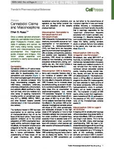
Char CNN

Char LSTM

(a) Character CNN.

B LSTM

F LSTM

(b) Character LSTM.

Figure 2: Neural character sequence representations. 3.1

Character Sequence Representations

Character features such as prefix, suffix and capitalization can be represented with embeddings through a feature-based lookup table (Collobert et al., 2011; Huang et al., 2015; Strubell et al., 2017), or neural networks without human-defined features (Lample et al., 2016; Ma and Hovy, 2016). In this work, we focus on neural character sequence representations without hand-engineered features. Character CNN. Using a CNN structure to encode character sequences was firstly proposed by Santos and Zadrozny (2014), and followed by many subsequent investigations (dos Santos et al., 2015; Chiu and Nichols, 2016; Ma and Hovy, 2016). In our experiments, we take the same structure as Ma and Hovy (2016), using one layer CNN structure with max-pooling to capture character-level representations. Figure 2(a) shows the CNN structure on representing word “Mexico”. Character LSTM. Shown as Figure 2(b), in order to model the global character sequence information of a word “Mexico”, we utilize a bidirectional LSTM on the character sequence of each word and concatenate the left-to-right final state FLST M and the right-to-left final state BLST M as character sequence representations. Liu et al. (2018) applied one bidirectional LSTM for the character sequence over a sentence rather than each word individually. We examined both structures and found that they give comparable accuracies on sequence labeling tasks. We choose Lample et al. (2016)’s structure as its character LSTMs can be calculated in parallel, making the system more efficient. 3.2

Word Sequence Representations

Similar to character sequences in words, we can model word sequence information through LSTM or CNN structures. LSTM has been widely used in sequence labeling (Lample et al., 2016; Ma and Hovy, 2016; Chiu and Nichols, 2016; Huang et al., 2015; Liu et al., 2018). CNN can be much faster than LSTM due to the fact that convolution calculation can be parallel on the input sequence (Collobert et al., 2011; dos Santos et al., 2015; Strubell et al., 2017). Word CNN. Figure 3(a) shows the multi-layer CNN on word sequence, where words are represented by embeddings. If a character sequence representation layer is used, then word embeddings and character sequence representations are concatenated for word representations. For each CNN layer, a window of size 3 slides along the sequence, extracting local features on the word inputs and a ReLU function (Glorot et al., 2011) is followed. We follow Strubell et al. (2017) by using 4 CNN layers. Batch normalization (Ioffe and Szegedy, 2015) and dropout (Srivastava et al., 2014) are applied following each CNN layer. Word LSTM. Shown in Figure 3(b), word representations are fed into a forward LSTM and backward LSTM, respectively. The forward LSTM captures the word sequence information from left to right, while the backward LSTM extracts information in a reversed direction. The hidden states of the forward and backward LSTMs are concatenated at each word to give global information of the whole sequence. 3.3

Inference Layer

The inference layer takes the extracted word sequence representations as features and assigns labels to the word sequence. Independent local decoding with a linear layer mapping word sequence representations

#Pad# COLING is

held

at

COLING

New Mexico #Pad#

is

held

at

New

O

BLOC

Mexico

Word Representations

Word Representations

Forward LSTM Backward LSTM

Multi-layer Convolutions

LSTM hidden

CNN hidden Softmax / CRF

O

O

O

O

(a) Word CNN.

BLOC

ELOC

Softmax / CRF

O

O

O

E LOC

(b) Word LSTM.

Figure 3: Neural word sequence representations. to label vocabulary and performing softmax can be quite effective (Ling et al., 2015), while for tasks that with strong output label dependency, such as NER, CRF is a more appropriate choice. In this work, we examine both softmax and CRF as inference layer on three sequence labeling tasks.

4

Experiments

We investigate the main influencing factors to system accuracy, including the character sequence representations, word sequence representations, inference algorithm, pretrained embeddings, tag scheme, running environment and optimizer; analyzing system performances from the perspective of decoding speed and accuracies on in-vocabulary (IV) and out-of-vocabulary (OOV) entities/chunks/words. 4.1

Settings

Data. The NER dataset has been standardly split in Tjong Kim Sang and De Meulder (2003). It contains four named entity types: P ERSON , L OCATION , O RGANIZATION , and M ISC. The chunking task is evaluated on CoNLL 2000 shared task (Tjong Kim Sang and Buchholz, 2000). We follow Reimers and Gurevych (2017a) by using sections 15-18 of Wall Street Journal (WSJ) for training, section 19 as development set and section 20 as test set. For the POS tagging task, we use the WSJ portion of Peen Treebank, which has 45 POS tags. Following previous works (Toutanova et al., 2003; Santos and Zadrozny, 2014; Ma and Hovy, 2016; Liu et al., 2018), we adopt the standard splits by using sections 0-18 as training set, sections 19-21 as development set and sections 22-24 as test set. No preprocessing is performed on either dataset except for normalizing digits. The dataset statistics are listed in Table 2. Hyperparameters. Table 3 shows the hyperparameters used in our experiments, which mostly follow Ma and Hovy (2016), including the learning rate η = 0.015 for word LSTM models. For word CNN based models, a large η leads to convergence problem. We take η = 0.005 with more epochs (200) instead. GloVe 100-dimension (Pennington et al., 2014) is used to initialize word embeddings and character embeddings are randomly initialized. We use mini-batch stochastic gradient descent (SGD) with a decayed learning rate to update parameters. For NER and chunking, we the BIOES tag scheme. Evaluation. Standard precision (P), recall (R) and F1-score (F) are used as the evaluation metrics for NER and chunking; token accuracy is used to evaluate the performance of POS tagger. Development datasets are used to select the optimal model among all epochs, and we report scores of the selected model on the test dataset. To reduce the volatility of the system, we conduct each experiment 5 times under different random seeds, and report the max, mean, and standard deviation for each model. 4.2

Results

Tables 4, 5 and 6 show the results of the twelve models on NER, chunking and POS datasets, respectively. Existing work has also been listed in the tables for comparison. To simplify the description, we use “CLSTM” and “CCNN” to represent character LSTM and character CNN encoder, respectively. Similarly, “WLSTM” and “WCNN” represent word LSTM and word CNN structure, respectively.

Dataset #Sent NER #Token #Entity #Sent chunking #Token #Chunk #Sent POS #Token

Train 14,987 205k 23,523 8,936 212k 107k 38,219 912k

Dev 3,644 52k 5,943 1,844 44k 22k 5,527 132k

Test 3,486 47k 5,654 2,012 47k 24k 5,462 130k

Label

Table 2: Statistics of datesets.

17

42 45

Parameter char emb size char hidden CNN window batch size L2 regularization λ word LSTM η word LSTM epochs

Value 30 50 3 10 1e-8 0.015 100

Parameter word emb size word hidden word CNN layer dropout rate learning rate decay word CNN η word CNN epochs

Value 100 200 4 0.5 0.05 0.005 200

Table 3: Hyperparameters.

As shown in Table 4, most NER work focuses on WLSTM+CRF structures with different character sequence representations. We re-implement the structure of several reports (Chiu and Nichols, 2016; Ma and Hovy, 2016; Peters et al., 2017), which take the CCNN+WLSTM+CRF architecture. Our reproduced models give slightly better performances. The results of Lample et al. (2016) can be reproduced by our CLSTM+WLSTM+CRF. In most cases, our “Nochar” based models underperform their corresponding prototypes (Huang et al., 2015; Strubell et al., 2017), which utilize the hand-crafted features. Table 5 shows the results of the chunking task. Peters et al. (2017) give the best reported single model results (95.00±0.08), and our CLSTM+WLSTM+CRF gives a comparable performance (94.93±0.05). We re-implement Zhai et al. (2017)’s model in our Nochar+WLSTM but cannot reproduce their results, this may because that they use grid search for hyperparameter selection. Our Nochar+WCNN+CRF can give comparable results with Collobert et al. (2011), even ours does not include character information. The results of the POS tagging task is shown in Table 6. The results of Lample et al. (2016), Ma and Hovy (2016) and Yang et al. (2017b) can be reproduced by our CLSTM+WLSTM+CRF and CCNN+WLSTM+CRF models. Our WLSTM based models give better results than WLSTM+CRF based models, this is consistent with the fact that Ling et al. (2015) take CLSTM+WLSTM without CRF layer but achieve the best POS accuracy. Santos and Zadrozny (2014) build a pure CNN structure on both character and word level, which can be reproduced by our CCNN+WCNN models. Based on above observations, most results in the literature are reproducible. Our implementations can achieve the comparable or better results with state-of-the-art models. We do not fine-tune any hyperparameter to fit the specific task. Results on Table 4, 5 and 6 are all under the same hyperparameters, which demonstrates the generalization ability of our framework. 4.3

Network settings

Character LSTM vs Character CNN. Unlike the observations of Reimers and Gurevych (2017b), in our experiments, character information can significantly (p < 0.01)3 improve sequence labeling models (by comparing the row of Nochar with CLSTM or CCNN on Table 4, 5 and 6), while the difference between CLSTM and CCNN is not significant. In most cases, CLSTM and CCNN can give comparable results under different frameworks and different tasks. CCNN gives the best NER result under the WLSTM+CRF framework, while CLSTM gets better NER results in all other configurations. For chunking and POS tagging, CLSTM consistently outperforms CCNN under all settings, while the difference is statistically insignificant (p > 0.2). We conclude that the difference between CLSTM and CCNN is small, which is consistent with the observation of Reimers and Gurevych (2017b). Word LSTM vs Word CNN. By comparing the performances of WLSTM+CRF, WLSTM with WCNN+CRF, WCNN on the three benchmarks, we conclude that word-based LSTM models are significantly (p < 0.01) better than word-based CNN models in most cases. It demonstrates that global word context information is necessary for sequence labeling. Softmax vs CRF. Models with CRF inference layer can consistently outperform the models with softmax layer under all configurations on NER and chunking tasks, proving the effectiveness of label dependency information. While for POS tagging, the local softmax based models give slightly better accuracies while the difference is insignificant (p > 0.2). 3

We use t-test to calculate the p value, reporting the highest p value when giving the conclusions on multiple configurations.

Results (F1-score) Literature Nochar Ours

Max Mean±std

Literature CLSTM Ours

Max Mean±std

Literature CCNN Ours

Max Mean±std

WLSTM+CRF 90.10 (H-15)* 90.20 (L-16) 90.43 (S-17)* 89.45 89.31±0.10 90.94 (L-16) 91.20 (Y-17)‡ 91.20 91.08±0.08 90.91±0.20 (C-16) 91.21 (M-16) 90.87±0.13 (P-17) 91.35 91.11±0.21

NER WLSTM WCNN+CRF 87.00 (M-16) 89.59 (C-11)* 89.34 (S-17)* 90.54 (S-17)*

WCNN 89.97 (S-17)*

88.57 88.49±0.17 89.15 (L-16)

88.90 88.65±0.20

88.56 88.50±0.05

–

–

90.84 90.77±0.06 89.36 (M-16)

90.70 90.48±0.23

90.46 90.28±0.30

–

–

90.43 90.28±0.09

90.51 90.26±0.19

90.73 90.60±0.11

Table 4: Results for NER.4 Results (F1-score) Literature Nochar Ours

Max Mean±std

Literature CLSTM

Max Mean±std Literature Max Ours Mean±std Ours

CCNN

WLSTM+CRF 94.46 (H-15)* 94.49 94.37±0.11 93.15 (R-17) 94.66 (Y-17)‡ 95.00 94.93±0.05 95.00±0.08 (P-17) 95.06 94.86±0.14

chunking WLSTM WCNN+CRF 94.13 (Z-17) 94.32 (C-11)* 95.02 (H-17)* 93.79 94.23 93.75±0.04 94.11±0.08

WCNN – 94.12 94.08±0.06

–

–

–

94.33 94.28±0.04 – 94.24 94.19±0.04

94.76 94.66±0.01 – 94.77 94.66±0.13

94.55 94.48±0.07 – 94.51 94.47±0.03

WCNN+CRF 97.29 (C-11)*

WCNN 96.13 (S-14)

96.99 96.95±0.04

97.07 97.01±0.04

–

–

97.38 97.33±0.03 – 97.33 97.29±0.03

97.38 97.33±0.04 97.32 (S-14) 97.33 97.30±0.02

Table 5: Results for chunking.4 Results (Accuracy) Literature Nochar Ours

Max Mean±std

Literature CLSTM

Max Mean±std Literature Max Ours Mean±std Ours

CCNN

WLSTM+CRF 97.55 (H-15)* 97.20 97.19±0.01 97.35±0.09 (L-16)† 97.55 (Y-17)‡ 97.49 97.47±0.02 97.55 (M-16) 97.46 97.43±0.02

POS WLSTM 96.93 (M-16) 97.45 (H-17)* 97.23 97.20±0.02 97.78 (L-15) 97.51 97.48±0.02 97.33 (M-16) 97.51 97.44±0.04

Table 6: Results for POS tagging.4

4 In Tables 4, 5 and 6, the abbreviation (C-11)=Collobert et al. (2011), (S-14)=Santos and Zadrozny (2014), (H-15)=Huang et al. (2015), (L-16)=Lample et al. (2016), (M-16)=Ma and Hovy (2016), (C-16)=Chiu and Nichols (2016), (Z-17)=Zhai et al. (2017), (H-17)=Hashimoto et al. (2017), (Y-17)=Yang et al. (2017b), (R-17)=Rei (2017), (S-17)=Strubell et al. (2017) and (P-17)=Peters et al. (2017). * suggests that models with handcrafted features. Results of (L-16)† is reported by Liu et al. (2018) by running the code of Lample et al. (2016) on the corresponding dataset. (Y-17)‡ use GRU for character and word sequence representations; here we regard GRU as a variant of LSTM.

90.71 90.54

91.11

CLSTM+WLSTM+CRF CCNN+WLSTM+CRF

90

91.2 91.08

88

91.0

F1-score

F1-score

91.11 92 91.08

86 83.37 83.36

84 GloVe

SENNA (a) Pretrained embeddings.

Random

CLSTM+WLSTM+CRF CCNN+WLSTM+CRF

91.03 91.00

90.91 90.82

90.8 90.6 GPU/BIOES

CPU

BIO

(b) Tag scheme and running environment.

Figure 4: Performance comparison on the CoNLL 2003 NER task. 4.4

External factors

In addition to model structures, external factors such as pretrained embeddings, tag scheme, and optimizer can significantly influence system performance. We investigate a set of external factors on the NER dataset with the two best models: CLSTM+WLSTM+CRF and CCNN+WLSTM+CRF. Pretrained embedding. Figure 4(a) shows the F1-scores of the two best models on the NER test set with two different pretrained embeddings, as well as the random initialization. Compared with the random initialization, models using pretrained embeddings give significant improvements (p < 0.01). The GloVe 100-dimension embeddings give higher F1-scores than SENNA (Collobert et al., 2011) on both models, which is consistent with the observation of Ma and Hovy (2016). Tag scheme. We examine two different tag schemes: BIO and BIOES (Ratinov and Roth, 2009). The results are shown in Figure 4(b). In our experiments, models using BIOES are significantly (p < 0.05) better than BIO. Our observation is consistent with most literature (Ratinov and Roth, 2009; Dai et al., 2015). Reimers and Gurevych (2017b) report that the difference between the schemes is insignificant. Running environment. Liu et al. (2018) observe that neural sequence labeling models can give better results on GPU rather than CPU. We conduct repeated experiments on both GPU and CPU environments. The results are shown in Figure 4(b). Models run on CPU give a lower mean F1-score than models run on GPU, while the difference is insignificant (p > 0.2). Optimizer. We compare different optimizers including SGD, Adagrad (Duchi et al., 2011), Adadelta (Zeiler, 2012), RMSProp (Tieleman and Hinton, 2012) and Adam (Kingma and Ba, 2014). The results are shown in Figure 55 . In contrast to Reimers and Gurevych (2017b), who reported that SGD is the worst optimizer, our results show that SGD outperforms all other optimizers significantly (p < 0.01), with a slower convergence process during training. Our observation is consistent with most literature (Chiu and Nichols, 2016; Lample et al., 2016; Ma and Hovy, 2016). 4.5

Analysis

Decoding speed. We test the decoding speeds of the twelve models on the NER dataset using a Nvidia GTX 1080 GPU. Figure 6 shows the decoding times on 10000 NER sentences. The CRF inference layer severely limits the decoding speed due to the left-to-right inference process, which disables the parallel decoding. Character LSTM significantly slows down the system. Compared with models without character information, adding character CNN representations does not affect the decoding speed too much but can give significant accuracy improvements (shown in Section 4.3). Due to the support of parallel computing, word-based CNN models are consistently faster than word-based LSTM models, with close accuracies, leading to large utilization potential in practice. 5

We fine-tune the learning rates for Adagrad, Adadelta, RMSProp and Adam, and report the best results in the figure.

91.11 91.08

90.84

F1-score

91.0

CLSTM+WLSTM+CRF CCNN+WLSTM+CRF

90.38 90.45 90.44

90.5 90.01 89.77

90.0

10 Time (s)

91.5

89.72 89.56

8

10.0

CLSTM CCNN Nochar

9.0 7.8 7.5

6

7.1

6.8

6.5

4.9 4.7 3.9 3.7

4

89.5 SGD Adagrad Adadelta RMSProp Adam Figure 5: Optimizers. Results Nochar+WLSTM+CRF CLSTM+WLSTM+CRF CCNN+WLSTM+CRF Nochar+WCNN+CRF CLSTM+WCNN+CRF CCNN+WCNN+CRF

IV 91.33 92.18 91.76 90.71 91.59 91.35

NER (F1-score) OOTV OOEV 87.36 100.00 90.63 100.00 91.25 100.00 86.99 100.00 90.07 100.00 90.46 100.00

6.1

WLSTM+CRF WLSTM WCNN+CRF WCNN Figure 6: Decoding times (10000 NER sentences).

OOBV 69.68 78.57 81.58 69.09 77.92 78.88

IV 94.87 95.20 95.15 94.56 95.02 94.83

chunking (F1-score) OOTV OOEV OOBV 90.84 95.51 91.47 92.65 94.38 94.01 92.34 97.75 93.55 90.98 93.26 91.71 91.86 94.38 93.32 92.42 96.63 92.40

IV 97.51 97.63 97.62 97.29 97.48 97.46

POS (Accuracy) OOTV OOEV 89.76 94.07 93.82 94.07 93.33 94.69 89.10 94.17 93.28 94.17 92.74 93.86

OOBV 75.36 87.32 83.82 74.15 88.29 87.80

Table 7: Results for OOV analysis. OOV error. We conduct error analysis on in-vocabulary and out-of-vocabulary words with the CRF based models6 . Following Ma and Hovy (2016), words in the test set are divided into four subsets: in-vocabulary words, out-of-training-vocabulary words (OOTV), out-of-embedding-vocabulary words (OOEV) and out-of-both-vocabulary words (OOBV). For NER and chunking, we consider entities or chunks rather than words. The OOV entities and chunks are categorized following Ma and Hovy (2016). Table 7 shows the performances of different OOV splits on three benchmarks. The top three rows list the performances of word-based LSTM CRF models, followed by the word-based CNN CRF models. The results of OOEV in NER keep 100% because of there exist only 8 OOEV entities and all are recognized correctly. It is obvious that character LSTM or CNN representations improve OOTV and OOBV the most on both WLSTM+CRF and WCNN+CRF models across all three datasets, proving that the main contribution of neural character sequence representations is to disambiguate the OOV words. Models with character LSTM representations give the best IV scores across all configurations, which may be because character LSTM can be well trained on IV data, bringing the useful global character sequence information. On the OOVs, character LSTM and CNN gives comparable results.

5

Conclusion

We built a unified neural sequence labeling framework to reproduce and compare recent state-of-theart models with different configurations. We explored three neural model design decisions: character sequence representations, word sequence representations, and inference layer. Experiments show that character information helps to improve model performances, especially on disambiguating OOV words. Character-level LSTM and CNN structures give comparable improvements, with the latter being more efficient. In most cases, models with word-level LSTM encoders outperform those with CNN, at the expense of longer decoding time. We observed that the CRF inference algorithm is effective on NER and chunking tasks, but does not have the advantage on POS tagging. With controlled experiments on the NER dataset, we showed that BIOES tags are better than BIO. Besides, pretrained GloVe 100d embedding and SGD optimizer give significantly better performances compared to their competitors. 6

We choose the models that give the median performance on the test set for conducting result analysis.

Acknowledgements We thank the anonymous reviewers for their useful comments. Yue Zhang is the corresponding author.

References Jason Chiu and Eric Nichols. 2016. Named entity recognition with bidirectional LSTM-CNNs. TACL, 4:357–370. Ronan Collobert, Jason Weston, L´eon Bottou, Michael Karlen, Koray Kavukcuoglu, and Pavel Kuksa. 2011. Natural language processing (almost) from scratch. Journal of Machine Learning Research, 12(Aug):2493– 2537. Hong-Jie Dai, Po-Ting Lai, Yung-Chun Chang, and Richard Tzong-Han Tsai. 2015. Enhancing of chemical compound and drug name recognition using representative tag scheme and fine-grained tokenization. Journal of cheminformatics, 7(S1):S14. Cıcero dos Santos, Victor Guimaraes, RJ Niter´oi, and Rio de Janeiro. 2015. Boosting named entity recognition with neural character embeddings. In Proceedings of NEWS 2015 The Fifth Named Entities Workshop, page 25. John Duchi, Elad Hazan, and Yoram Singer. 2011. Adaptive subgradient methods for online learning and stochastic optimization. Journal of Machine Learning Research, 12(Jul):2121–2159. Xavier Glorot, Antoine Bordes, and Yoshua Bengio. 2011. Deep sparse rectifier neural networks. In Proceedings of the Fourteenth International Conference on Artificial Intelligence and Statistics, pages 315–323. James Hammerton. 2003. Named entity recognition with long short-term memory. In Proceedings of the seventh conference on Natural language learning at HLT-NAACL 2003-Volume 4, pages 172–175. Association for Computational Linguistics. Kazuma Hashimoto, Yoshimasa Tsuruoka, Richard Socher, et al. 2017. A joint many-task model: Growing a neural network for multiple nlp tasks. In Proceedings of the 2017 Conference on Empirical Methods in Natural Language Processing, pages 1923–1933. Zhiheng Huang, Wei Xu, and Kai Yu. 2015. Bidirectional LSTM-CRF models for sequence tagging. arXiv preprint arXiv:1508.01991. Sergey Ioffe and Christian Szegedy. 2015. Batch normalization: Accelerating deep network training by reducing internal covariate shift. In International conference on machine learning, pages 448–456. Diederik P Kingma and Jimmy Ba. 2014. Adam: A method for stochastic optimization. arXiv preprint arXiv:1412.6980. Guillaume Lample, Miguel Ballesteros, Sandeep Subramanian, Kazuya Kawakami, and Chris Dyer. 2016. Neural architectures for named entity recognition. In NAACL-HLT, pages 260–270. Yann LeCun, Bernhard Boser, John S Denker, Donnie Henderson, Richard E Howard, Wayne Hubbard, and Lawrence D Jackel. 1989. Backpropagation applied to handwritten zip code recognition. Neural computation, 1(4):541–551. Wang Ling, Chris Dyer, Alan W Black, Isabel Trancoso, Ramon Fermandez, Silvio Amir, Luis Marujo, and Tiago Luis. 2015. Finding function in form: Compositional character models for open vocabulary word representation. In Proceedings of the 2015 Conference on Empirical Methods in Natural Language Processing, pages 1520–1530. Liyuan Liu, Jingbo Shang, Frank Xu, Xiang Ren, Huan Gui, Jian Peng, and Jiawei Han. 2018. Empower sequence labeling with task-aware neural language model. AAAI. Gang Luo, Xiaojiang Huang, Chin-Yew Lin, and Zaiqing Nie. 2015. Joint entity recognition and disambiguation. In EMNLP, pages 879–888. Xuezhe Ma and Eduard Hovy. 2016. End-to-end sequence labeling via Bi-directional LSTM-CNNs-CRF. In ACL, volume 1, pages 1064–1074. Mitchell P Marcus, Mary Ann Marcinkiewicz, and Beatrice Santorini. 1993. Building a large annotated corpus of english: The penn treebank. Computational linguistics, 19(2):313–330.

Tomas Mikolov, Ilya Sutskever, Kai Chen, Greg S Corrado, and Jeff Dean. 2013. Distributed representations of words and phrases and their compositionality. In Advances in neural information processing systems, pages 3111–3119. Alexandre Passos, Vineet Kumar, and Andrew McCallum. 2014. Lexicon infused phrase embeddings for named entity resolution. In CoNLL, pages 78–86. Jeffrey Pennington, Richard Socher, and Christopher Manning. 2014. Glove: Global vectors for word representation. In Proceedings of the 2014 conference on empirical methods in natural language processing (EMNLP), pages 1532–1543. Matthew Peters, Waleed Ammar, Chandra Bhagavatula, and Russell Power. 2017. Semi-supervised sequence tagging with bidirectional language models. In ACL, volume 1, pages 1756–1765. Lev Ratinov and Dan Roth. 2009. Design challenges and misconceptions in named entity recognition. In CoNLL, pages 147–155. Marek Rei. 2017. Semi-supervised multitask learning for sequence labeling. In Proceedings of the 55th Annual Meeting of the Association for Computational Linguistics (Volume 1: Long Papers), volume 1, pages 2121– 2130. Nils Reimers and Iryna Gurevych. 2017a. Optimal hyperparameters for deep lstm-networks for sequence labeling tasks. arXiv preprint arXiv:1707.06799. Nils Reimers and Iryna Gurevych. 2017b. Reporting score distributions makes a difference: Performance study of lstm-networks for sequence tagging. In Proceedings of the 2017 Conference on Empirical Methods in Natural Language Processing, pages 338–348. Cicero D Santos and Bianca Zadrozny. 2014. Learning character-level representations for part-of-speech tagging. In Proceedings of the 31st International Conference on Machine Learning (ICML-14), pages 1818–1826. Nitish Srivastava, Geoffrey E Hinton, Alex Krizhevsky, Ilya Sutskever, and Ruslan Salakhutdinov. 2014. Dropout: a simple way to prevent neural networks from overfitting. Journal of Machine Learning Research, 15(1):1929– 1958. Emma Strubell, Patrick Verga, David Belanger, and Andrew McCallum. 2017. Fast and accurate entity recognition with iterated dilated convolutions. In Proceedings of the 2017 Conference on Empirical Methods in Natural Language Processing, pages 2670–2680. Tijmen Tieleman and Geoffrey Hinton. 2012. Lecture 6.5-rmsprop: Divide the gradient by a running average of its recent magnitude. COURSERA: Neural networks for machine learning, 4(2):26–31. Erik F Tjong Kim Sang and Sabine Buchholz. 2000. Introduction to the conll-2000 shared task: Chunking. In Proceedings of the 2nd workshop on Learning language in logic and the 4th conference on Computational natural language learning-Volume 7, pages 127–132. Association for Computational Linguistics. Erik F Tjong Kim Sang and Fien De Meulder. 2003. Introduction to the conll-2003 shared task: Languageindependent named entity recognition. In HLT-NAACL, pages 142–147. Kristina Toutanova, Dan Klein, Christopher D Manning, and Yoram Singer. 2003. Feature-rich part-of-speech tagging with a cyclic dependency network. In Proceedings of the 2003 Conference of the North American Chapter of the Association for Computational Linguistics on Human Language Technology-Volume 1, pages 173–180. Association for Computational Linguistics. Zhilin Yang, Ruslan Salakhutdinov, and William Cohen. 2016. Multi-task cross-lingual sequence tagging from scratch. arXiv preprint arXiv:1603.06270. Jie Yang, Yue Zhang, and Fei Dong. 2017a. Neural reranking for named entity recognition. In Proceedings of the International Conference Recent Advances in Natural Language Processing, RANLP 2017, pages 784–792. Zhilin Yang, Ruslan Salakhutdinov, and William W Cohen. 2017b. Transfer learning for sequence tagging with hierarchical recurrent networks. In ICLR. Matthew D Zeiler. 2012. Adadelta: an adaptive learning rate method. arXiv preprint arXiv:1212.5701. Feifei Zhai, Saloni Potdar, Bing Xiang, and Bowen Zhou. 2017. Neural models for sequence chunking. In AAAI, pages 3365–3371.